In this work, we considered the practical applications of our method, thus the simulation and physical tests were designed to verify the algorithm. The experiments are processed in two cases, which are the swaying case and the in-motion case. Three traditional methods, which are applied in practical systems, are designed for comparison. They are as follows: (i) the traditional apparent gravitational method, which is represented as Scheme 1 [
20]; (ii) the digital filter method, which is represented as Scheme 2 [
23]; and (iii) the in-motion method based on the apparent velocity, which is denoted as Velocity Integration Formula (VIF) method [
18]. The proposed method in this paper is denoted as Scheme 3.
6.1. Simulation Tests on the Swaying Base
In this subsection, a simulation test for the swaying base is studied. The sawing rule is
, and
and
are the amplititude and frequency of the swaying motion, while
and
represent the initial phase and swaying center, respectively. The swaying parameters for the test are listed in
Table 2.
The whole coarse alignment of this test lasts for 600 s, and the geographic latitude and longitude of the vehicle are set as
and
. By using the aforementioned parameters, the outputs of the inertial sensors can be collected by the back-stepping algorithm of the SINS solution. Then, the coarse alignment results can be calculated by the generated outputs of the inertial sensors. In this simulation, the sensor errors are set in
Table 3.
Without loss of generality, the initial parameters matrix
is set as a 3 × 3 null matrix, and the initial estimation error covariance matrix is set as
, and the adaptive measurement noise is set as
. The robust filter threshold
is equal to 0.05 in the simulation test. The simulation results of the swaying motion are shown in
Figure 6,
Figure 7 and
Figure 8, and the estimated parameters matrix
is shown in
Figure 6. The observation vectors, which are employed to different methods, are depicted in
Figure 7, while the alignment errors of four methods are shown in
Figure 8.
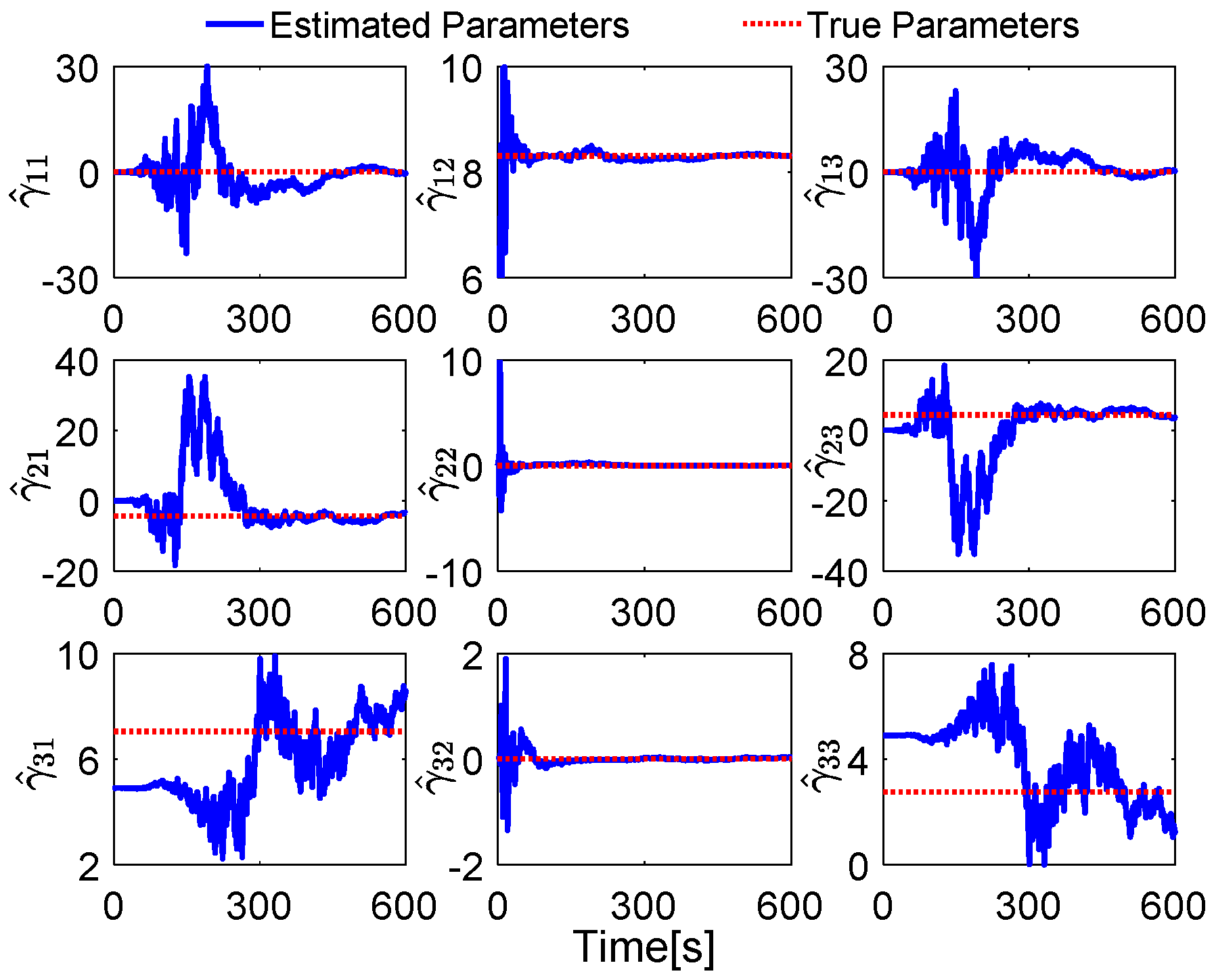
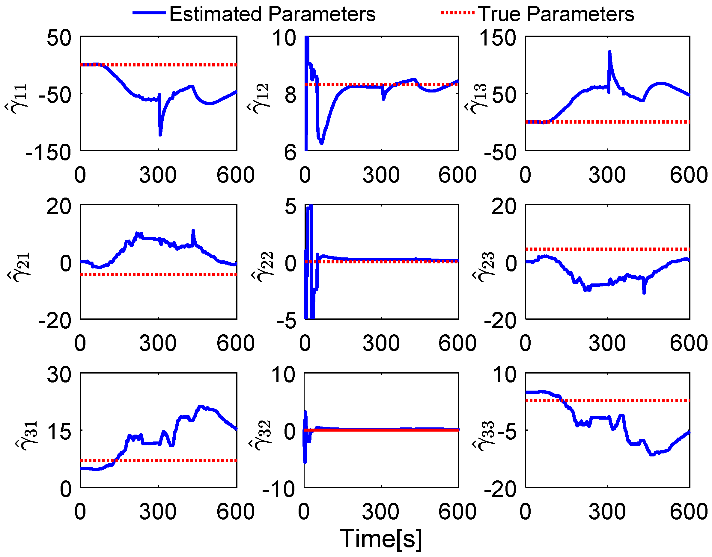
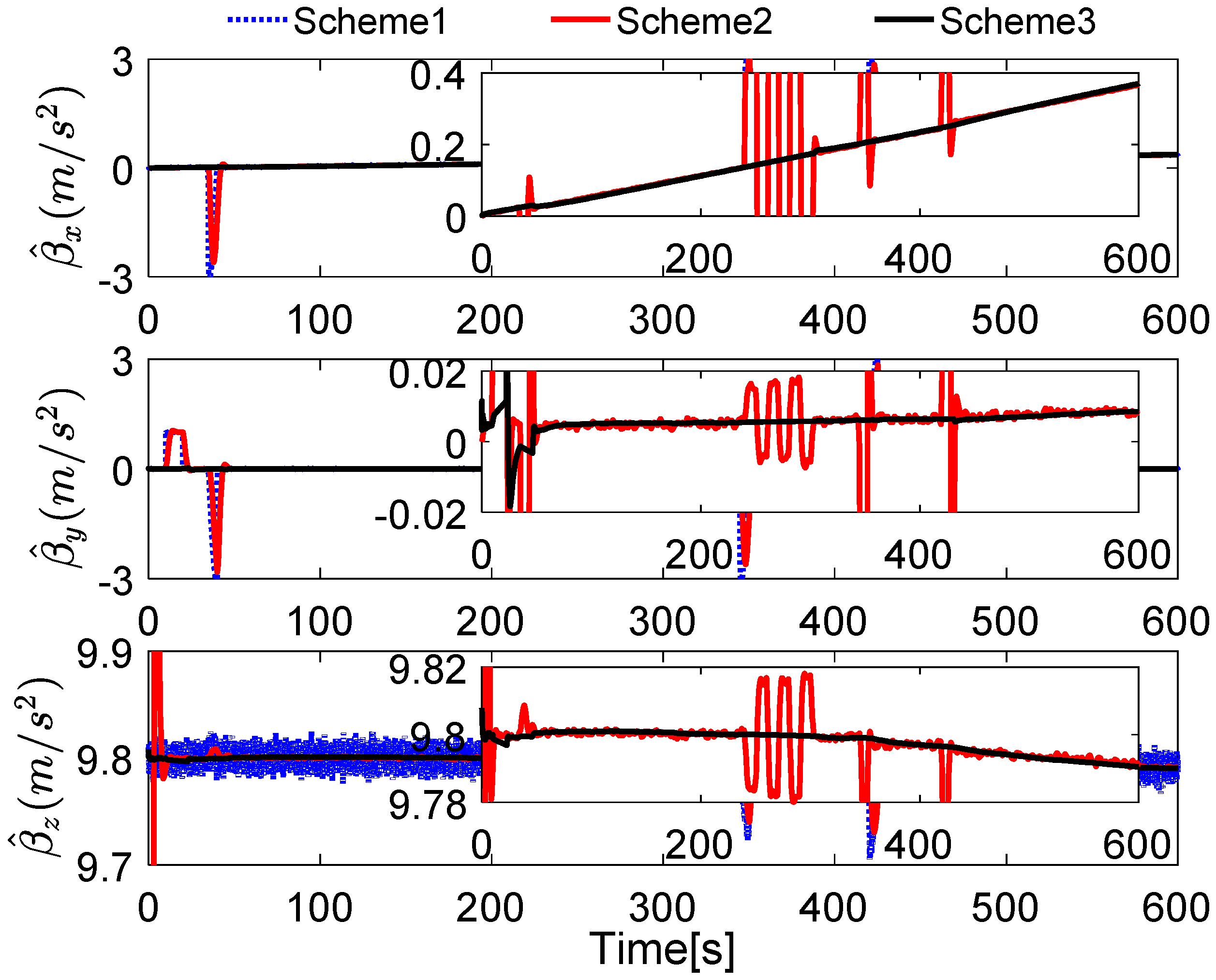
In
Figure 6, the red dotted line represents the true parameters and the blue line denotes the estimated parameters. Since the initial attitude is set as
at start up, the DCM
is equal to the 3 × 3 identity matrix, and the true parameter matrix is shown in Equation (18). It can be found that the second parameters of each row of
have a faster convergence rate, while the first and the third ones have wide fluctuation; these features are reasonable because the second element in each row of
is the main components of the reconstructed observation vectors, and the small components are consisted with the first and the third elements in each row of
, when the initial attitude is set as
at start up.
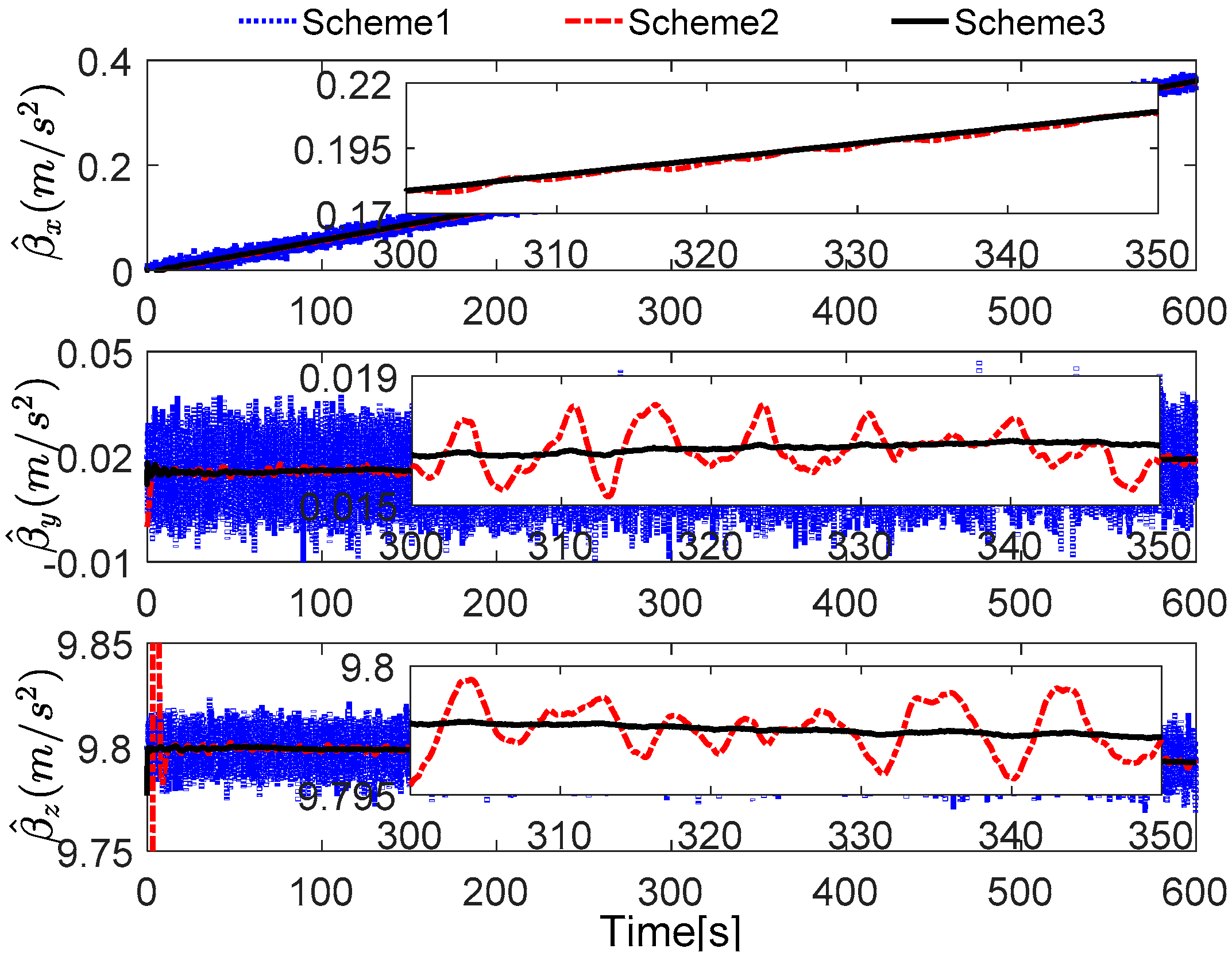
In
Figure 7, the reconstructed observation vectors of Scheme 3 has confirmed our aforementioned analysis, and they are smoothed. Due to the existing noises and the defects of the digital filter, the observation vectors of Scheme 1 and Scheme 2 are fluctuant, but it also can be notes that many high-frequency noises have be eliminated in Scheme 2. These different features will influence the performance of coarse alignment directly.
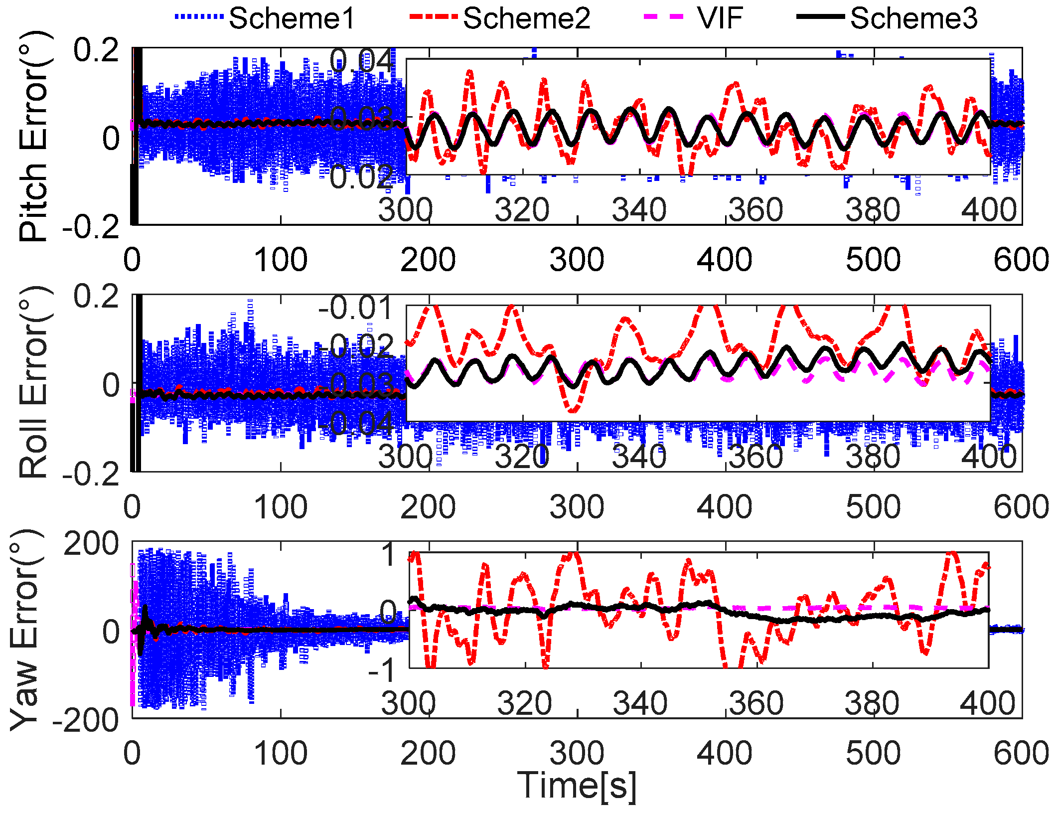
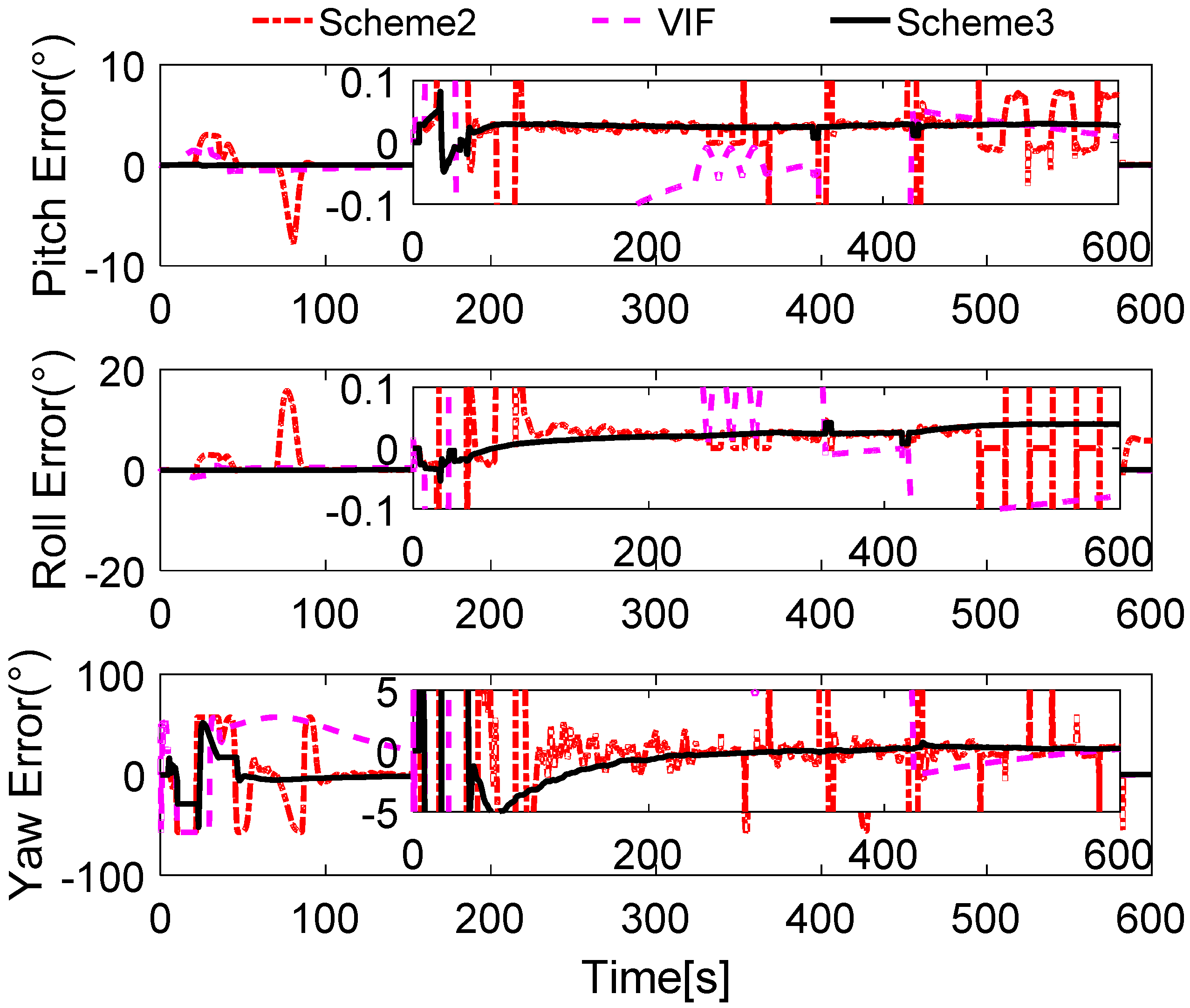
In
Figure 8, it is shown that the alignment results of Scheme 3 are more stable than Scheme 1 and Scheme 2, and are equivalent to the current VIF method, which is based on apparent velocity. For convenient comparison, the partial enlarged views of the alignment errors between 300 s and 400 s are depicted, where the errors of Scheme 1 have been ignored due to the wide fluctuation.
To verify our analysis, the statistics of three methods between 300 s and 400 s are listed in
Table 4. It can be obviously found that the mean values of the errors of horizontal angles are closer, which are around 0.028° for pitch error and −0.025° for roll error. However, as the STD value shows, the horizontal angles of three methods error of Scheme 3 and VIF method are around 0.0020°, while the horizontal angles error of Scheme 2 is greater than 0.004°, which is more than twice as much as the other two methods. In the yaw errors, the same features can be found. This reveals that the results of Scheme 2 are unstable, and the performance of Scheme 2 will decline in the harsh external environment. It can be also noted that the STD value of yaw errors of Scheme 3 is 0.0904°, while that of the VIF method is 0.0098°, which is much smaller than Scheme 3. This is because the apparent gravity are more sensitive to the external noises than the apparent velocity, and the simulation condition are ideal. In the practical cases, there always exist linear velocity disturbation, then Scheme 3 will be better than the VIF method. This is verified in the next subsections.
6.2. Simulation Tests for the Vehicle Motion
In the swaying simulation, it is shown that the performance of Scheme 3 is better than Scheme 2, and it is equivalent to the VIF method. In this work, the application of the initial alignment under the in-motion base is considered, and the simulation for the vehicle test is designed in this subsection. In
Table 5, the state of the vehicle motion is listed, the curves of the vehicle motion are depicted in
Figure 9.
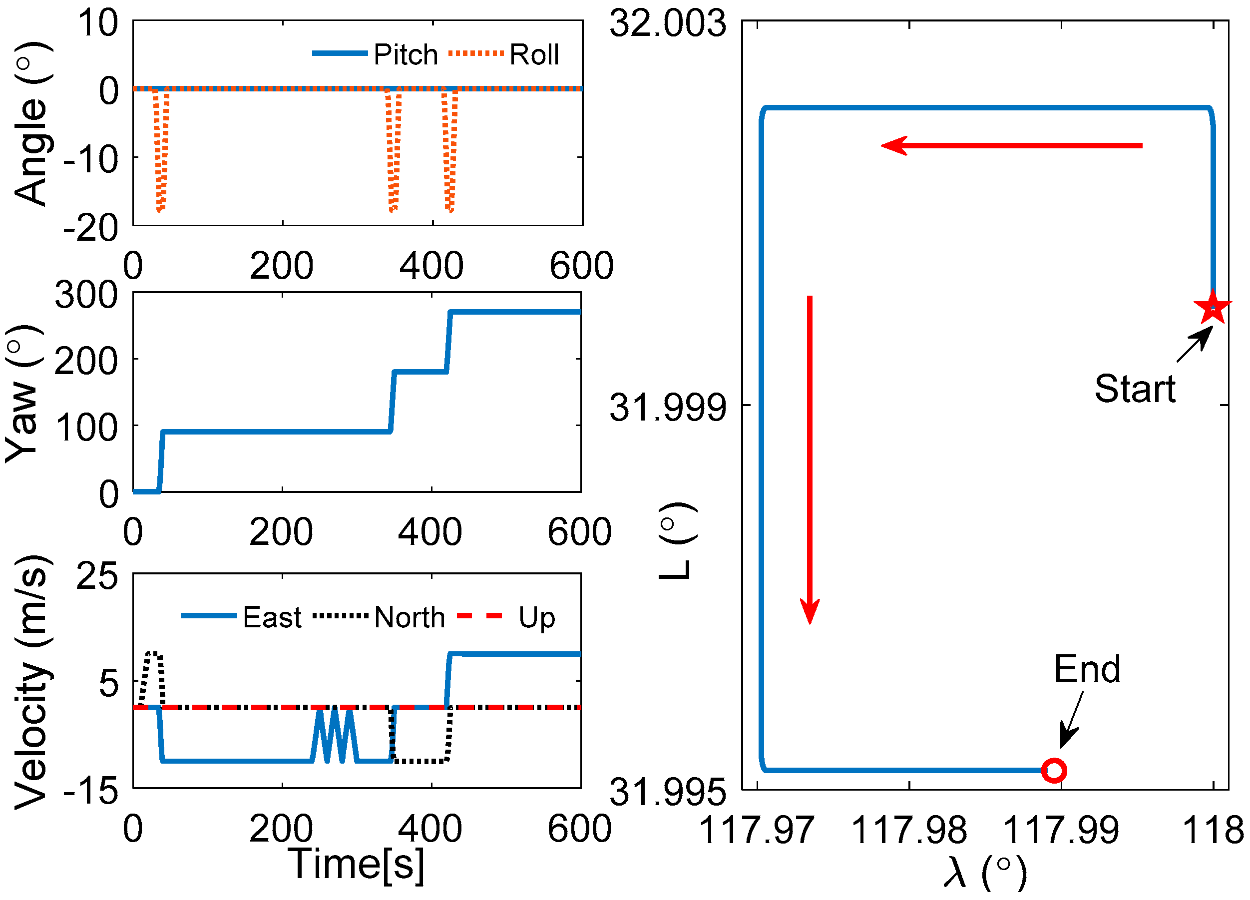
To verify the proposed method effectively, the common in-motion states of the vehicle, such as acceleration, deceleration, uniform motion, and turning motion, are considered. In this simulation, the velocity of the vehicle is lower than 10 m/s, and the rotating speed is 6°/s, which are the relative proper in-motion cases for initial alignment. Under the cases of this movement, the outputs of the inertial sensors can be acquired, and the alignment results are shown in
Figure 10,
Figure 11 and
Figure 12. In
Figure 10, the curves of vehicle motion is depicted, they are attitude, velocity, and the well-defined trajectory. It is obvious that the moving velocity of the simulation test is not higher than 10 m/s, because the much higher velocity will contaminate the performance of this coarse alignment.
Due to the well-known initial condition of the vehicle, the true parameters are certain. In
Figure 10, the estimated parameter matrix is depicted, and the familiar features can be found in
Figure 6. As shown, the second parameter of each row of
is close to the true parameter, the fluctuation is small, while the other six parameters are wide fluctuations; the reasons have been analyzed in
Section 6.1. It is also noted that the parameter
is tuning during the whole alignment. This is caused by the real correction of the robust filter, when the new effective measurements are acquired after some outliers, the parameters will be re-estimated. In addition, the other two parameters
and
are smoother than
; this is because the gravitational apparent motion is projected on
, and the parameters
and
are not sensitive to the measurements. The analysis has been confirmed with the reconstructed observation vectors, which is calculated by Equation (32).
In
Figure 11, the reconstructed observation vectors of Schemes 1–3 are shown. It can be found that the digital filter cannot eliminate the outliers caused by the vehicle motion, but the robust filter, which is proposed by this paper, can address these defects effectively. It can also be noted that the reconstructed observation vectors
have significant changes, which consisted of the aforementioned analysis.
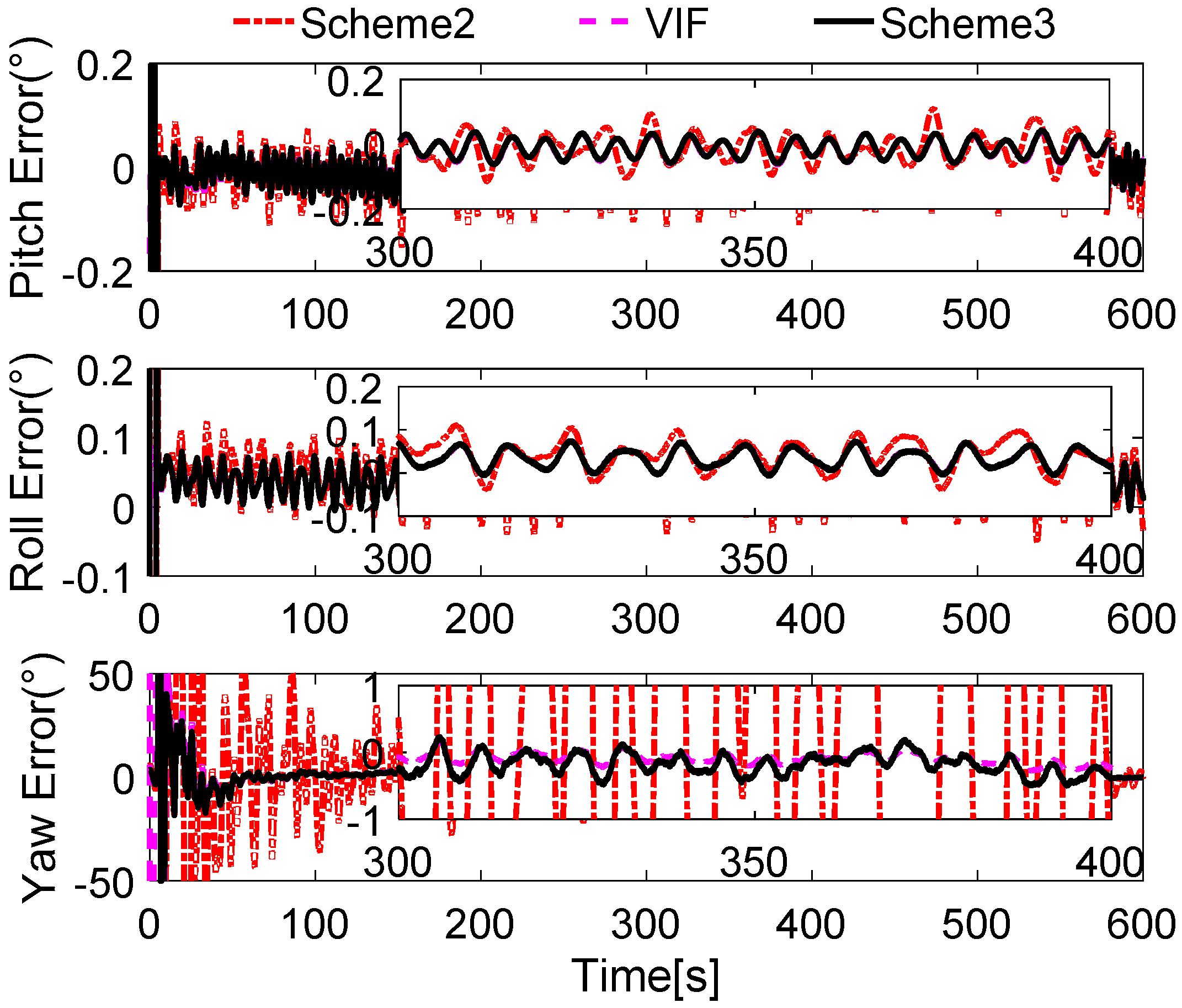
In
Figure 12, the alignment errors are described. Due to the greater errors in Scheme 1, we do not depict the alignment results of Scheme 1. During the 600 s coarse alignment, the results of Scheme 2 and the VIF method are fluctuating, and they are sensitive to the vehicle motion, thus the results are not suitable for the follow-on inertial navigation. By using the more precisely reconstructed observation vectors, the alignment results of the proposed method are steady and accurate.
For showing the performance of the proposed method, the statistics of the alignment errors during the whole alignment procedure are listed in
Table 6.
The statistics of the alignment errors of the proposed method show that the mean value of the final errors of horizontal angles is less than 0.05°, and the STD value is under 0.01°. When the coarse alignment procedure lasts for 600 s, the mean value of the yaw errors is around 0.2°, and the corresponding STD value is under 0.2°. All of the errors are low enough for the fine alignment.
6.3. Turntable Test
To verify the performance of the proposed method in practical applications, the practical tests, including the turntable test and field vehicle test are designed in this subsection and the next subsection, respectively.
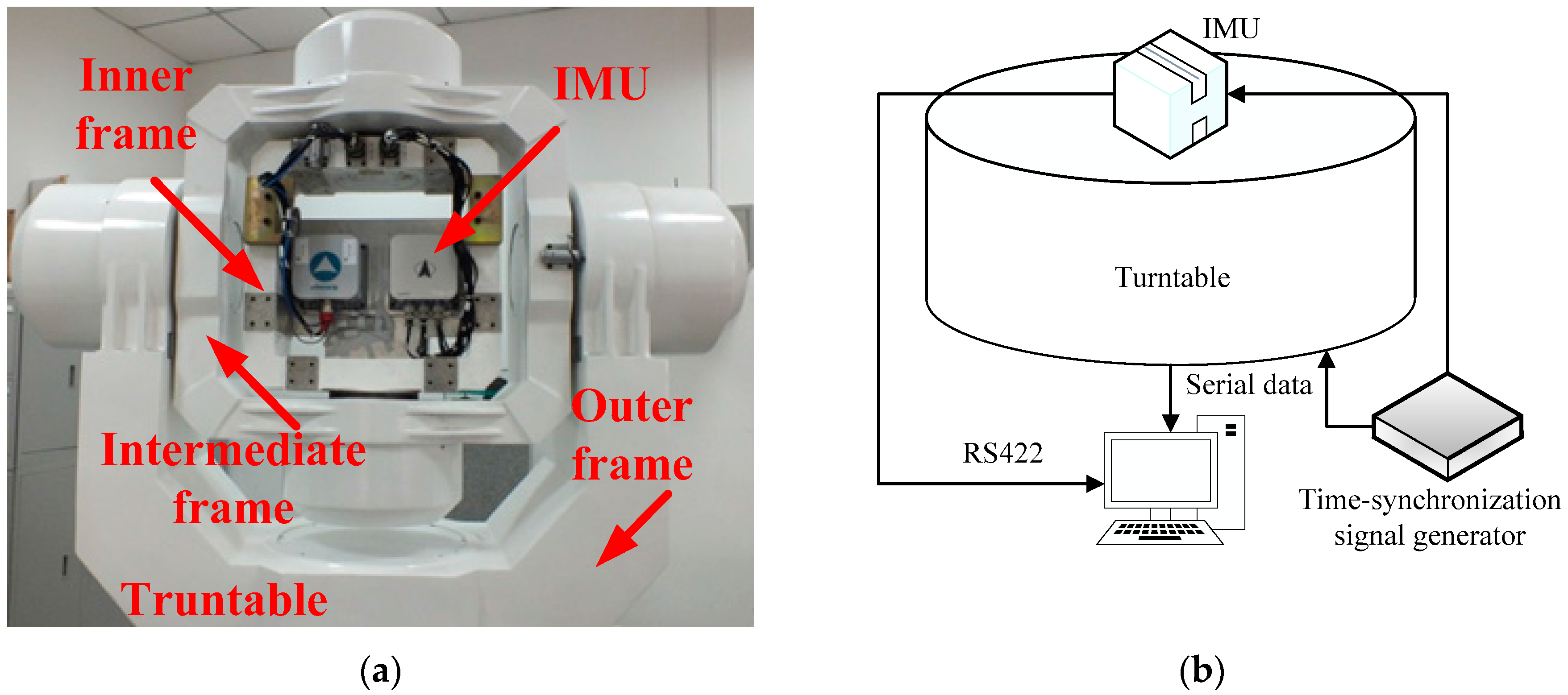
For the turntable test, the equipment is installed as shown in
Figure 13a, and the construction of the turntable test is as shown in
Figure 13b. The turntable is designed by the AVIC Beijing Precision Engineering Institute for the aircraft industry, and the controlling accuracy is ±0.0005°/s, the accuracy of the corresponding angle controlling is ±0.0001°. The IMU used in this test is a navigational-grade production, the corresponding parameters are listed in
Table 7.
In this test, the data from turntable and SINS is collected via serial communication ports as a response to the external time-synchronization signal. Before the test, all of the system errors, such as the coupling coincident scale factors of the inertial sensors, installing errors, and so on, are corrected by the calibration test, so the above-mentioned system errors are ignored.
The outputs rate of the turntable and SINS are set as 200 Hz, and the turntable works under the swaying condition, the swaying parameters are as common as
Table 2. The Kalman filter parameters are set, as shown in
Section 6.1, and the robust filter parameter in this test is set as
, because the magnitude of the noises are greater than the simulation tests. The coarse alignment also lasts for 600 s, the reconstructed observation vectors and the alignment errors are depicted in
Figure 14 and
Figure 15, respectively.
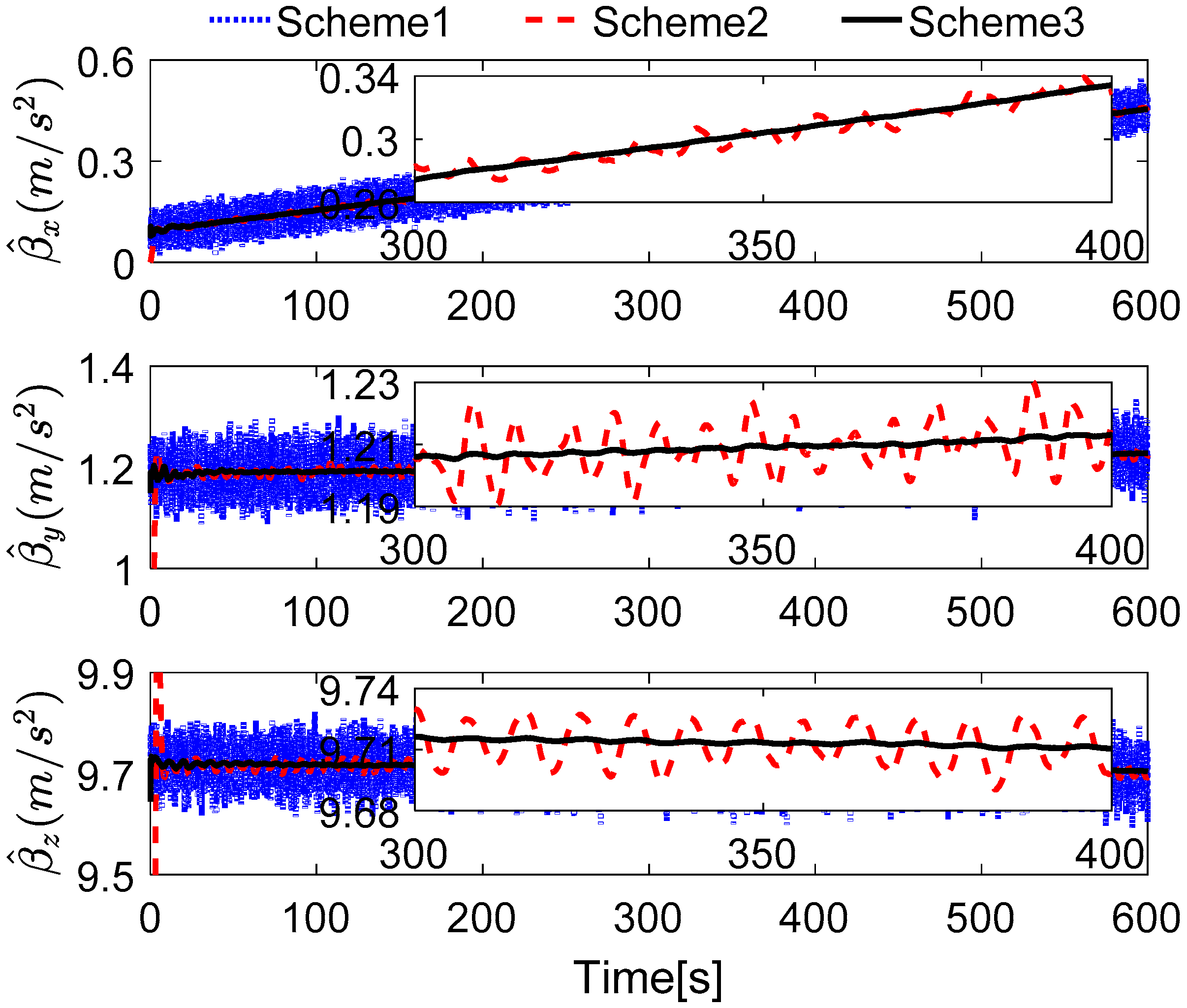
In
Figure 14, it can be found that the reconstructed observation vectors based on Scheme 2 are widely fluctuating, which is caused by the drawbacks of the low-pass digital filter. It is obvious that the reconstructed observation vector, which is acquired by Scheme 3, is smoother than Scheme 2. In addition, it is easily concluded that the smoother observation vector will acquire more stable alignment results, so the alignment results of Scheme 3 will be smoother than Scheme 2.
In
Figure 15, the results of Scheme 1 are ignored due to the great interference of the reconstructed observation vectors in
Figure 14. The alignment errors are showed that the performance of Scheme 3 is superior to Scheme 2, because the reconstructed observation vectors of Scheme 2 are more widely fluctuating than that which are reconstructed by Scheme 3. Just like in
Section 6.1, the partially enlarged views of the alignment errors between 300 s and 400 s are depicted in
Figure 15, it can be found that the performance of Scheme 2 is inferior to Scheme 3 and the VIF method, and the horizontal performance of Scheme 3 are familiar with the VIF method. For clear analysis, the statistics of the alignment errors of the three methods from 300 s and 400 s are listed in
Table 8.
In
Table 8, the mean value of pitch and roll errors of three methods are approximated. However, the STD values of VIF and Scheme 3 are around 0.02
°, it is smaller than Scheme 2, which is larger than 0.03
°. Due to the smoothed feature of reconstructed observation vector of Scheme 3, it can be found that the STD value of the yaw error of Scheme 3 is 0.1543
°, while it is 5.2979
° of Scheme 2. These features reveal that the alignment results of Scheme 2 are unstable, thus the digital filter cannot obtain the excellent results. Based on the apparent velocity properties, the STD value of the VIF method is 0.1222
°, and the corresponding value of Scheme 3 is 0.1543
°. Moreover, the mean value of yaw error of Scheme 3 is −0.1696°, which is −0.1424° for the VIF. It is revealed that the performance of VIF and Scheme 3 is quite equivalent. However, when the alignment is processing under the in-motion case without additional information, Scheme 3 will be superior to the VIF method, and this test is investigated in the next subsection.
6.4. Vehicle Test
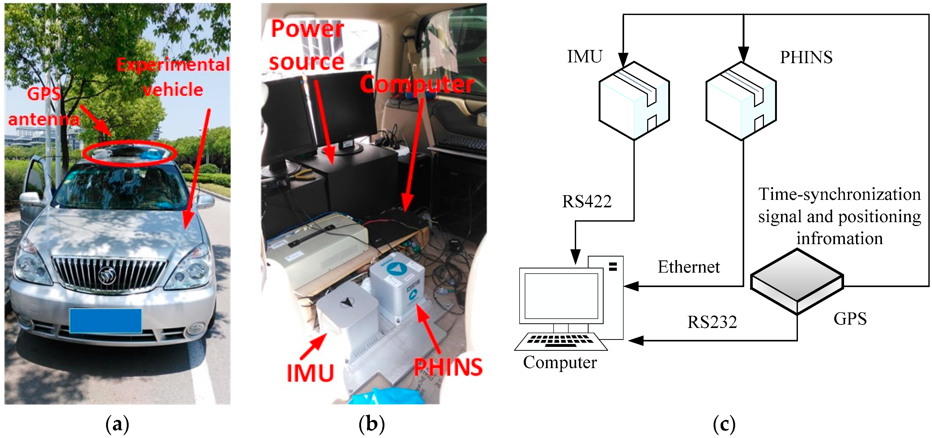
In this subsection, the field vehicle test of coarse alignment is designed for examining the performance of Scheme 3. PHINS III, which is produced by iXBlue Corporation (Saint-Germain en Laye Cedex, France), is utilized as the reference system. The experimental vehicle, installed IMU and PHINS and construction of vehicle test are shown in
Figure 16a–c, respectively. In
Figure 16a, a GPS antenna is used to collect the GPS signal, which is required for PHINS, and then the initial position of the vehicle is well-known. In
Figure 16b, the IMU and PHINS are installed on the surface of a steel plate, and the power is supplied with a rechargeable battery pack. All of the raw data of the sensors are logged by the computer. Moreover, a real-time operation system (VxWorks) is embedded in the navigation computer. Four methods mentioned in this paper are processed by four real-time tasks of VxWorks. The alignment results are also logged by the computer.
Figure 16c gives the construction of the vehicle test, and the outputs of GPS provide the time-synchronization signal for IMU and PHINS. The positioning information of GPS is also acquired by PHINS and computers via serial communication ports. The PHINS data are collected via Ethernet, and the raw data of the outputs of the inertial sensors are transferred via an RS422 port.
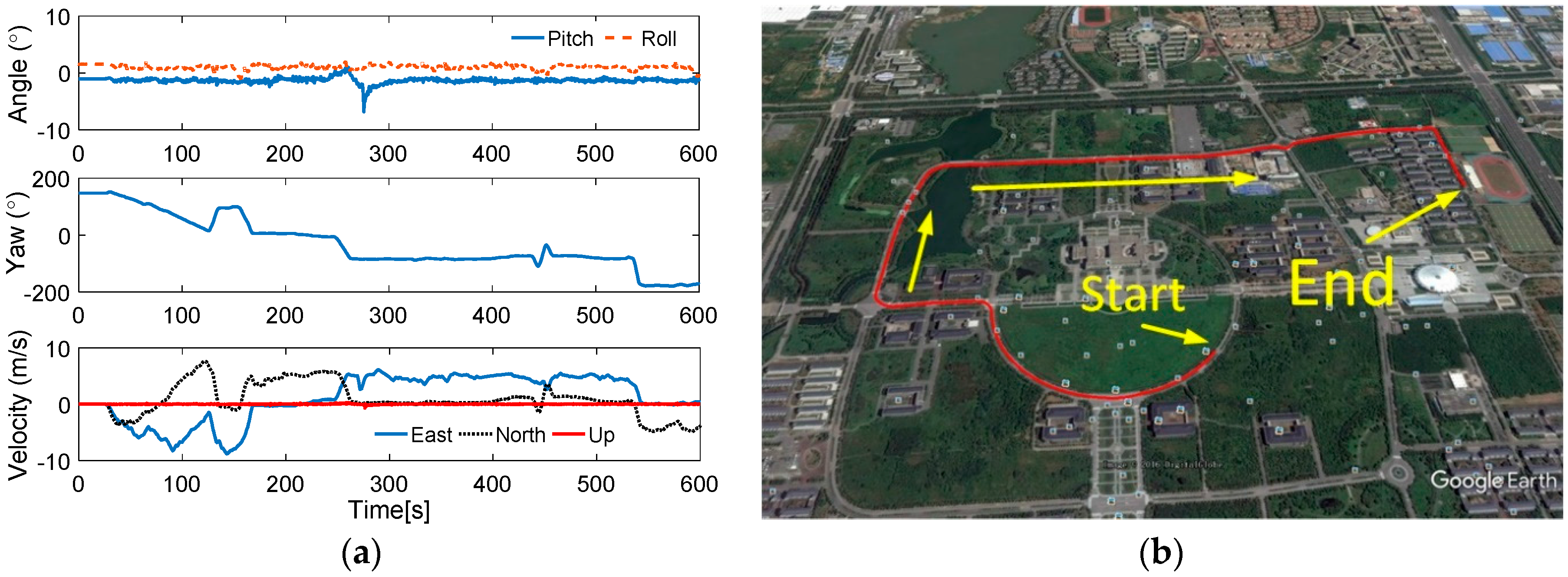
Before the test, the installed error between IMU and PHINS are corrected, and the IMU system errors, such as the coupling coincident scale factors of the inertial sensors, are also corrected by the calibration methods. In
Figure 17, the curves and trajectory of vehicle motion are depicted, and the field test is proceeded on our campus. The velocity of the vehicle is under 10 m/s.
The field test designed here lasts for 600 s, and the reconstructed observation vectors and the alignment errors are shown in
Figure 18 and
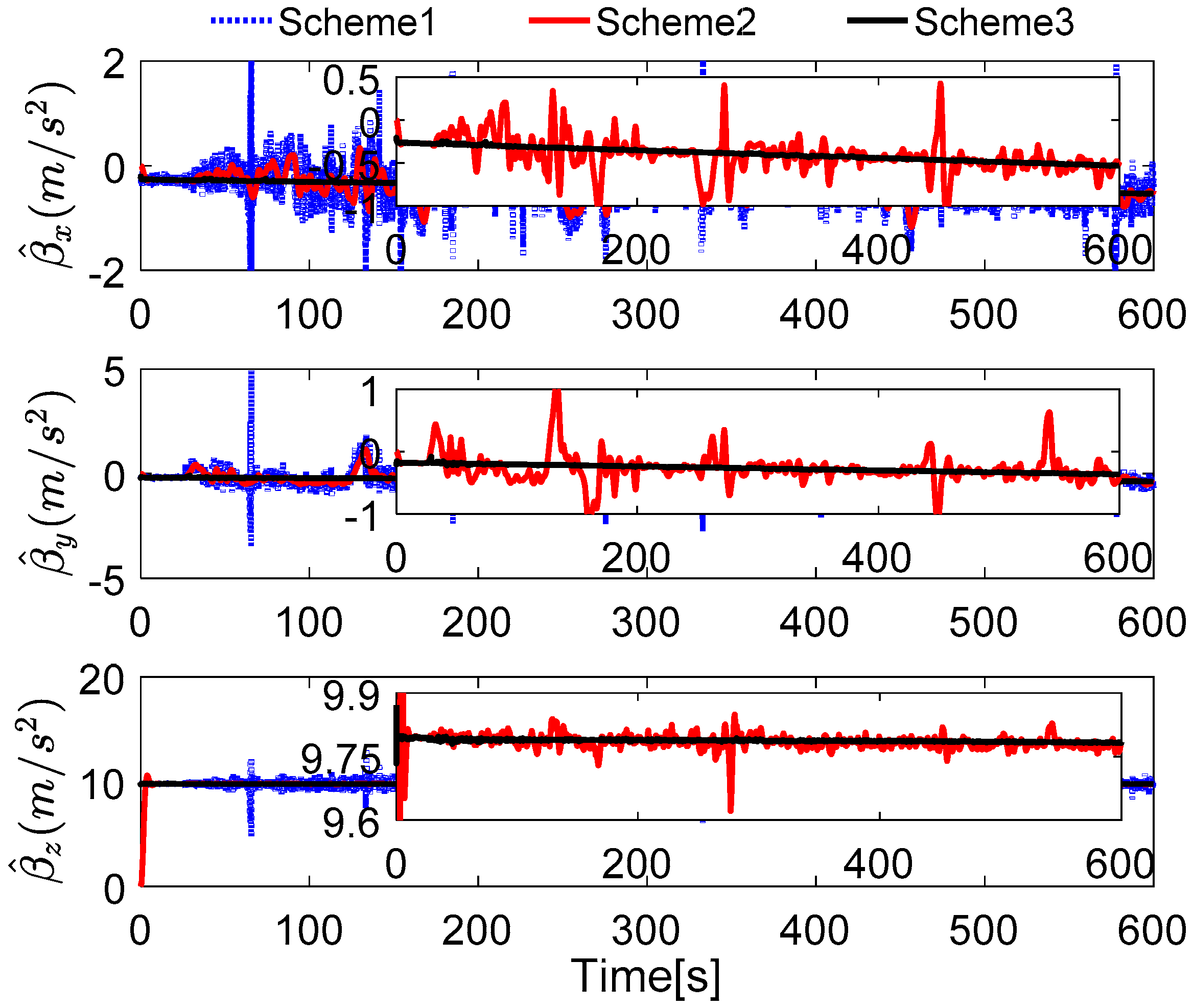
Figure 19, respectively. In
Figure 18, the reconstructed observation vectors of the three methods are shown, and the wide fluctuation in Scheme 1 can be found, which is because the disturbance of the vehicle movement, the external environment, and the sensors’ noises. Based on the IIR low-pass digital filter, some high-frequency noises are filtered out from the observation vectors. The enlarged views of the reconstructed observation vectors are shown that there are a lot of outliers in Scheme 2, these outliers will contaminate the performance of the coarse alignment. Based on Scheme 3, the outliers are address by the robust filter, and the optimal observation vectors are extracted by the parameter recognition and the reconstruction algorithm, which shows that the reconstructed observation vectors of Scheme 3 are more stable. The alignment errors showed in
Figure 19 also verify the precision of the extracted observation vectors of Scheme 3.
In
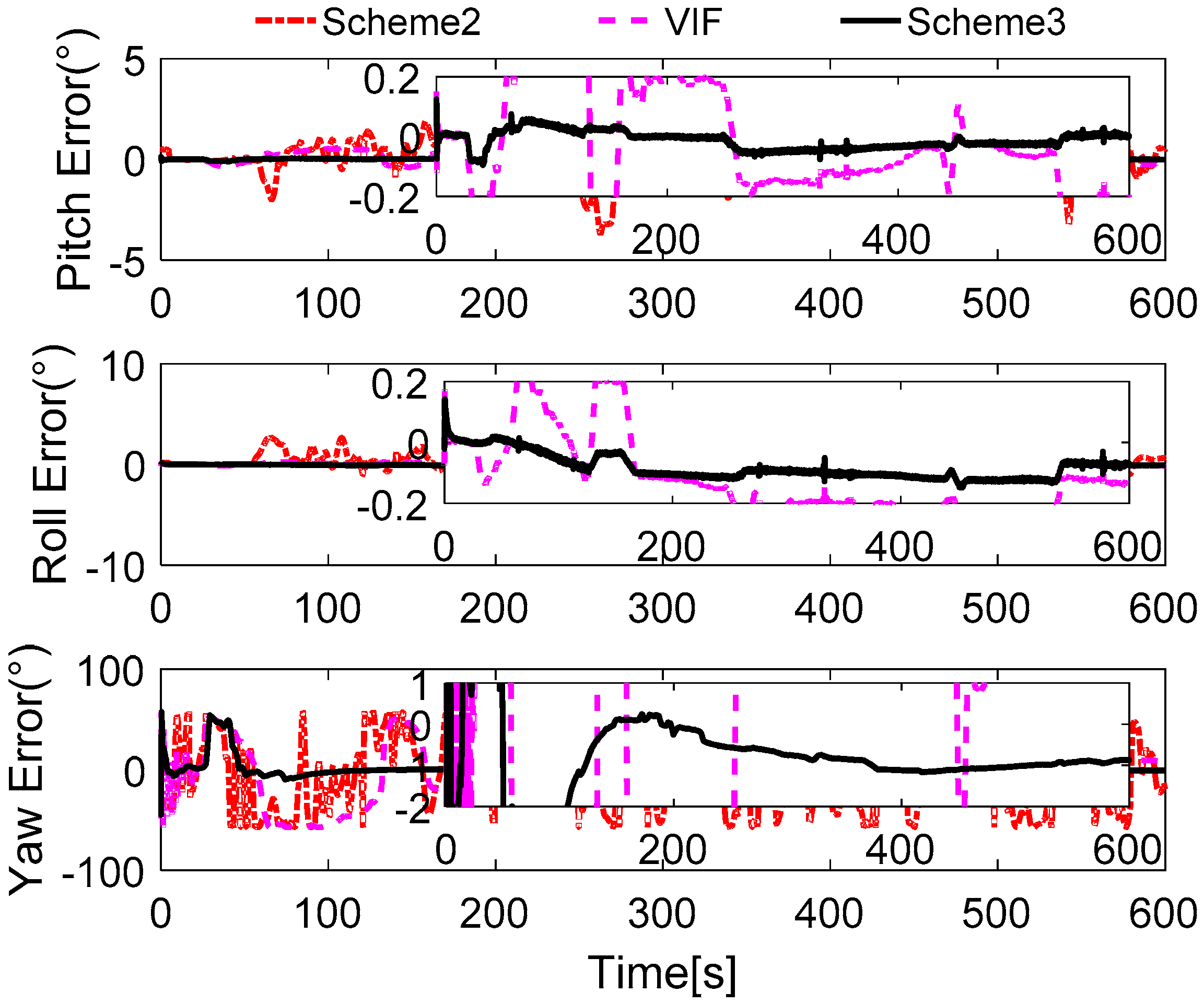
Figure 19, it is obviously found that the alignment results of Scheme 2 are wide fluctuation and it does not acquired a stable value after 600 s. In this test, the SINS under an entirely self-contained mode is considered. Hence, the performance of the VIF method is also poor in this field test, because the additional information, which is the external reference velocity, cannot be acquired when SINS is under an entirely self-contained mode. According to the aforementioned analysis, the reconstructed observation vectors of Scheme 3 have been reconstructed by the designed method, and the precision of these vectors can be verified by the alignment errors. It is noted that the performance of Scheme 3 is superior to the other two methods, and the errors of pitch and roll are less than 0.2° during the whole alignment procedure. The errors of yaw are constraint in 2°, when the errors are stable. It is also can be found that the smaller distortion of the alignment errors of Scheme 3, and this is caused by the interference of the vehicle movements, which disturb the measurement observation vectors. In order to show the precision of Scheme 3,
Table 9 summarized the statistics of the alignment errors of Scheme 3.
In
Table 9, it is shown that the STD value of the errors of pitch and roll are less than 0.1°, and the corresponding value of yaw errors is less than 0.5° after the alignment lasts for 100 s. These reveal that the alignment results of Scheme 3 are available in the practical system.


