Benthic Habitat Mapping Using Multispectral High-Resolution Imagery: Evaluation of Shallow Water Atmospheric Correction Techniques


Abstract
1. Introduction
2. Methodology
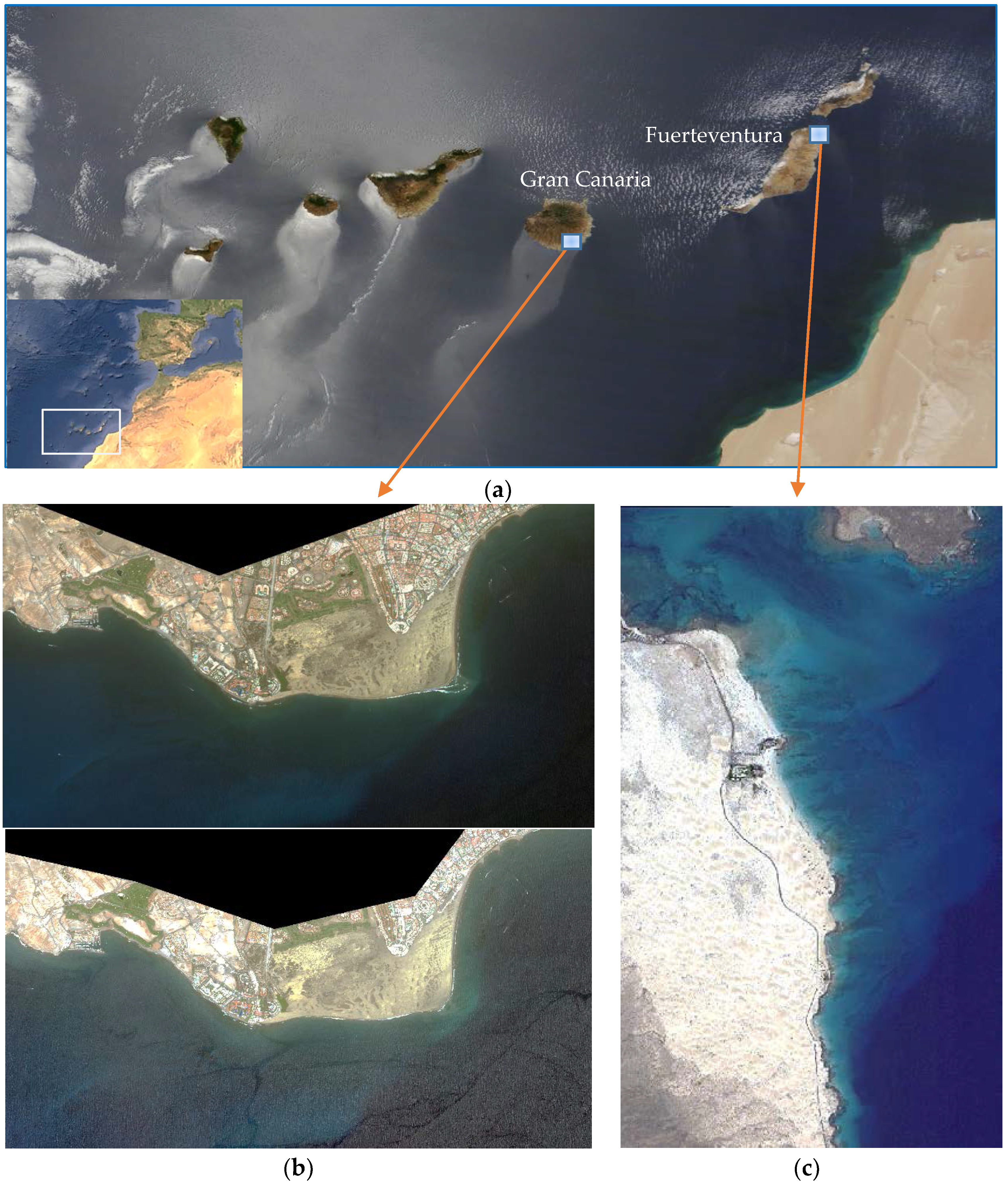
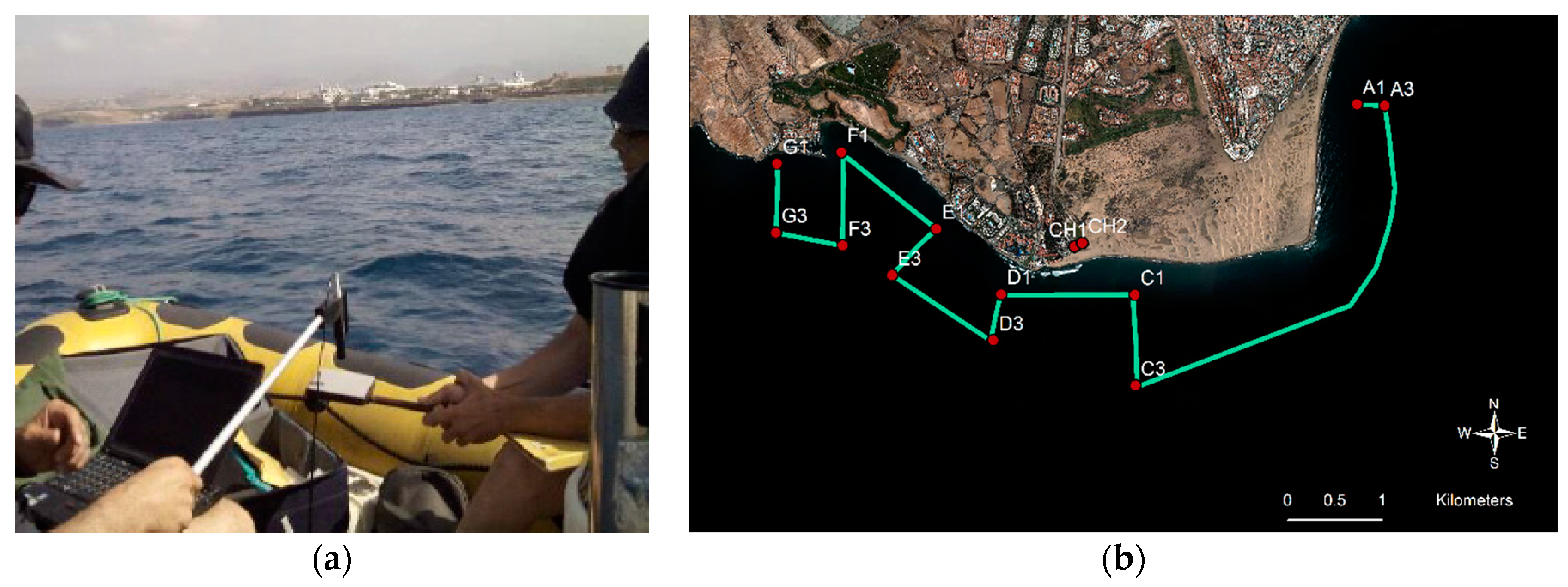
2.1. Dataset and Study Area
2.2. Multispectral High-Resolution Data Correction
2.2.1 Atmospheric Correction Algorithms
- represents the difference between solar and satellite azimuth.
- represents the total transmissibility of the gases (in the upward and downward path), taking into account the absorption of the different gases of the atmosphere.
- represents the atmospheric reflectivity, which depends on the molecular properties and the aerosols in the atmosphere.
- represents the atmospheric thickness (Atmospheric Optical Depth, AOD).
- represents the diffuse transmittance of the atmosphere.
- represents the spherical albedo of the atmosphere.
- The term takes into account the multiple scatterings between the surface and the atmosphere. As it can be seen, the absorption and scattering processes are dealt separately in the 6S equation. The scattering produced by molecules and aerosols are differentiated as well. The total reflectivity of the atmosphere is obtained by the introduction of coefficients from Rayleigh scattering and aerosols. These coefficients are obtained by first-order approximations.
- (i)
- The Mid-Latitude Summer seems the most suitable atmosphere model for the climate of the Canary Islands. Water vapor was considered implicitly when selecting the atmosphere model as it considers standard column water vapor amounts (from sea level to space).
- (ii)
- The most acceptable aerosol model for the islands is the Maritime model.
- (iii)
- The aerosol optical thickness (AOT) parameter must be properly adjusted using in-situ or satellite information because major errors in their estimation can significantly affect the surface reflectivity computed. Nowadays, such information is daily available from satellite sensors (i.e., MODIS at 550 nm).
2.2.2. Automatic Correction of Sunglint Effect
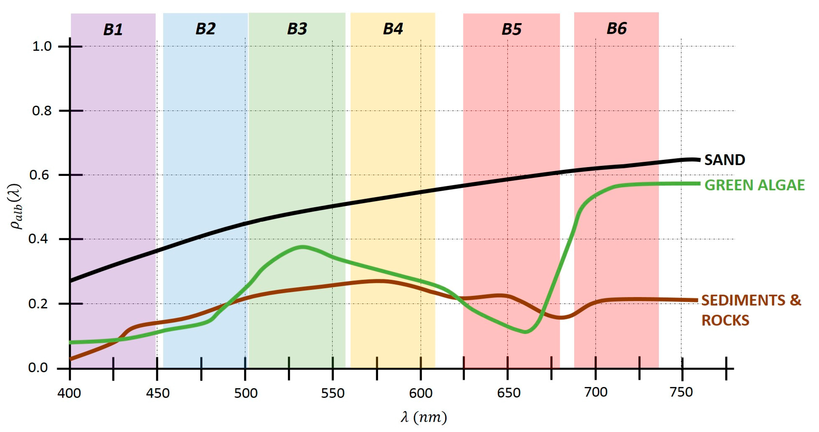
2.3. Coastal Monitoring Algorithms: Benthic Habitat Abundance Mapping and Bathymetry Estimation
3. Results and Discussion
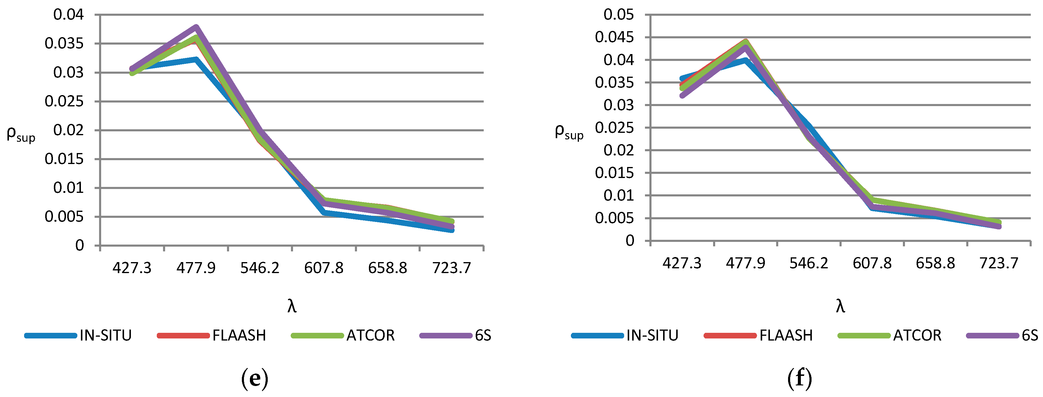
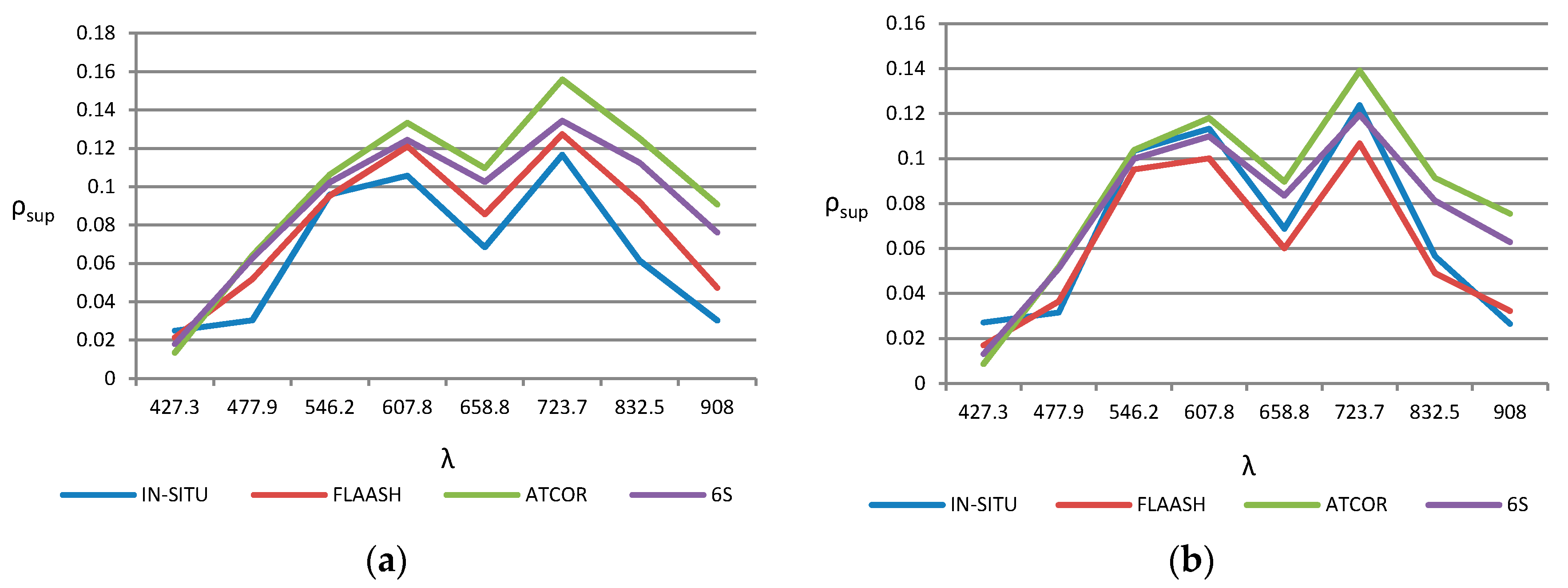
3.1. Atmosperic Assessment: Absolute Evaluation Using In-situ Spectroradiometer Measurements
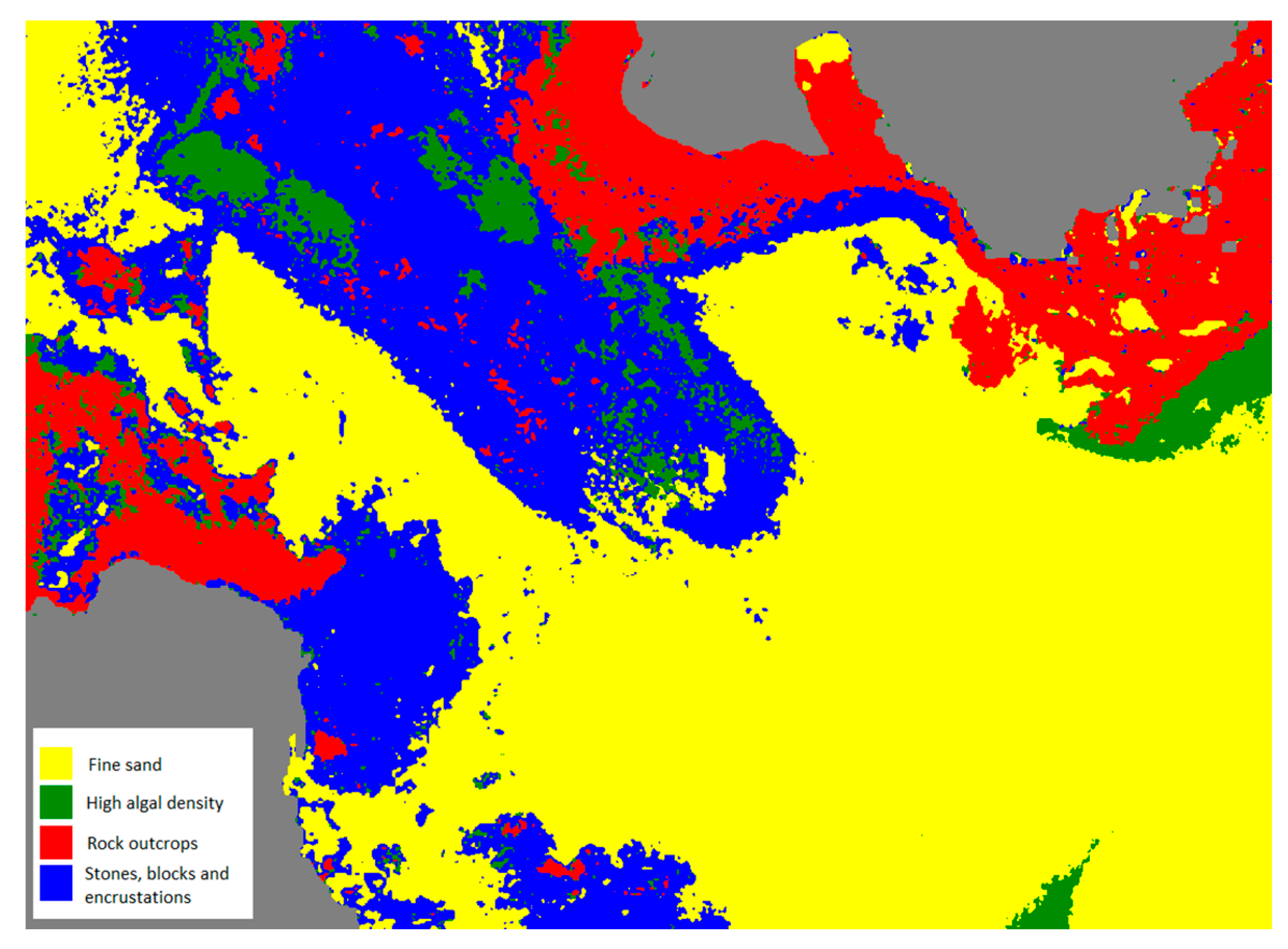
3.2. Coastal Monitoring: Benthos Abundance
4. Conclusions
Acknowledgments
Author Contributions
Conflicts of Interest
References
- Horning, E.; Robinson, J.; Sterling, E.; Turner, W.; Spector, S. Remote Sensing for Ecology and Conservation; Oxford University Press: New York, NY, USA, 2010. [Google Scholar]
- Wang, Y. Remote Sensing of Coastal Environments; Taylor and Francis Series; CRC Press: Boca Raton, FL, USA, 2010. [Google Scholar]
- Richards, J.A. Remote Sensing Digital Image Analysis; Springer: Berlin, Germany, 2013. [Google Scholar]
- Lyons, M.; Phinn, S.; Roelfsema, C. Integrating Quickbird multi-spectral satellite and field data: Mapping bathymetry, seagrass cover, seagrass species and change in Moreton bay, Australia in 2004 and 2007. Remote Sens. 2011, 3, 42–64. [Google Scholar] [CrossRef]
- Knudby, A.; Nordlund, L. Remote Sensing of Seagrasses in a Patchy Multi-Species Environment. Int. J. Remote Sens. 2011, 32, 2227–2244. [Google Scholar] [CrossRef]
- ZhongPing, L.; Casey, B.; Arnone, R.; Weidemann, A.; Parsons, R.; Montes, M.; Gao, B.C.; Goode, W.; Davis, C.O.; Dyef, J. Water and bottom properties of a coastal environment derived from Hyperion data measured from the EO-1 spacecraft platform. J. Appl. Remote Sens. 2007, 1. [Google Scholar] [CrossRef]
- Kibele, J.; Shears, N.T. Nonparametric Empirical Depth Regression for Bathymetric Mapping in Coastal Waters. IEEE J. Sel. Top. Appl. Earth Obs. Remote Sens. 2016, 9, 5130–5138. [Google Scholar] [CrossRef]
- Adler-Golden, S.M.; Acharya, P.A.; Berk, A.; Matthew, M.; Gorodetzky, D. Remote bathymetry of the littoral zone from AVIRIS, LASH and QuickBird imagery. IEEE Trans. Geosci. Remote Sens. 2005, 43, 337–347. [Google Scholar] [CrossRef]
- Sokoletsky, L.G.; Fang, S. Optical closure for remote-sensing reflectance based on accurate radiative transfer approximations: The case of the Changjiang (Yangtze) River Estuary and its adjacent coastal area, China. Int. J. Remote Sens. 2014, 35, 4193–4224. [Google Scholar] [CrossRef]
- Collin, A.; Hench, J.L. Towards deeper measurements of tropical reefscape structure using the WorldView-2 spaceborne sensor. Remote Sens. 2012, 4, 1425–1447. [Google Scholar] [CrossRef]
- Eugenio, F.; Marcello, J.; Martin, J. High-resolution maps of bathymetry and benthic habitats in shallow-water environments using multispectral remote sensing imagery. IEEE Trans. Geosci. Remote Sens. 2015, 53, 3539–3549. [Google Scholar] [CrossRef]
- Hadjimitsis, D.G.; Clayton, C.; Hope, V.S. An assessment of the effectiveness of atmospheric correction algorithms through the remote sensing of some reservoirs. Int. J. Remote Sensi. 2004, 25, 18. [Google Scholar] [CrossRef]
- Mahiny, A.S.; Turner, B.J. A comparison of four common atmospheric correction methods. Photogramm. Eng. Remote Sens. 2007, 73, 361–368. [Google Scholar] [CrossRef]
- Smith, G.M.; Milton, E.J. The use of the empirical line method to calibrate remotely sensed data to reflectance. Int. J. Remote Sens. 1999, 20, 2653–2662. [Google Scholar] [CrossRef]
- Wu, J.; Wang, D.; Bauer, M.E. Image-based atmospheric correction of QuickBird imagery of Minnesota cropland. Remote Sens. Environ. 2005, 99, 315–325. [Google Scholar] [CrossRef]
- Nguyen, H.C.; Jung, J.; Lee, J.; Choi, S.U.; Hong, S.Y.; Heo, J. Optimal Atmospheric Correction for Above-Ground Forest Biomass Estimation with the ETM+ Remote Sensor. Sensors 2015, 15, 18865–18886. [Google Scholar] [CrossRef] [PubMed]
- Broszeit, A.; Ashraf, S. Using different atmospheric correction methods to classify remotely sensed data to detect liquefaction of the February 2011 earthquake in Christchurch. In Proceedings of the GIS and Remote Sensing Research Conference, Dunedin, New Zealand, 29–30 August 2013. [Google Scholar]
- Agrawal, G.; Sarup, J. Comparison of QUAC and FLAASH Atmospheric Correction Modules on EO-1 Hyperion Data of Sanchi. Int. J. Adv. Eng. Sci. Technol. 2011, 6, 178–186. [Google Scholar]
- Pu, R.; Landry, S.; Zhang, J. Evaluation of Atmospheric Correction Methods in Identifying Urban Tree Species with WorldView-2 Imagery. IEEE J. Sel. Top. Appl. Earth Obs. Remote Sens. 2015, 8, 1886–1897. [Google Scholar] [CrossRef]
- Vanonckelen, S.; Lhermitte, S.; Van Rompaey, A. The effect of atmospheric and topographic correction methods on land cover classification accuracy. Int. J. Appl. Earth Obs. Geoinf. 2013, 24, 9–21. [Google Scholar] [CrossRef]
- El Hajj, M.; Bégué, A.; Lafrance, B.; Hagolle, O.; Dedieu, G.; Rumeau, M. Relative Radiometric Normalization and Atmospheric Correction of a SPOT 5 Time Series. Sensors 2008, 8, 2774–2791. [Google Scholar] [CrossRef] [PubMed]
- Marcello, J.; Eugenio, F.; Perdomo, U.; Medina, A. Assessment of Atmospheric Algorithms to Retrieve Vegetation in Natural Protected Areas Using Multispectral High-resolution Imagery. Sensors 2016, 16, 1624. [Google Scholar] [CrossRef] [PubMed]
- Martin, J.; Medina, A.; Eugenio, F.; Marcello, J.; Bermejo, J.A.; Arbelo, M. Atmospheric Correction for high-resolution images WorldView-2 using 6S model, a case study in the Canary Islands, Spain. In Proceedings of the SPIE Remote Sensing Europe, Edinburgh, UK, 24–27 September 2012. [Google Scholar]
- Pacifici, F. An automatic atmospheric compensation algorithm for very high spatial resolution imagery and its comparison to FLAASH and QUAC. In Proceedings of the Joint Agency Commercial Imagery Evaluation (JACIE) Workshop, Saint Louis, MO, USA, 16–18 April 2013. [Google Scholar]
- San, B.T.; Suzen, M.L. Evaluation of different atmospheric correction algorithms for EO-1 Hyperion imagery. International Archives of the Photogrammetry. Remote Sens. Spat. Inf. Sci. 2010, 38, 392–397. [Google Scholar]
- Kay, S.; Hedley, J.; Lavender, S. Sun glint correction of high and low spatial resolution images of aquatic scenes: A review of methods for visible and near-infrared wavelengths. Remote Sens. 2009, 1, 697–730. [Google Scholar] [CrossRef]
- Lyzenga, D.R.; Malinas, N.P.; Tanis, F.J. Multispectral bathymetry using a simple physically based algorithm. IEEE Trans. Geosci. Remote Sens. 2006, 44, 2251–2259. [Google Scholar] [CrossRef]
- Martin, J.; Eugenio, F.; Marcello, J.; Medina, A. Automatic Sunglint Removal of Multispectral High-Resolution Worldview-2 Imagery for Retrieving Coastal Shallow Water Parameters. Remote Sens. 2016, 8, 37. [Google Scholar] [CrossRef]
- Morel, A. Optical modeling of the upper ocean in relation to its biogenous matter content (case I waters). J. Geophys. Res. Oceans 1988, 93, 10749–10768. [Google Scholar] [CrossRef]
- DigitalGlobe, Inc. Available online: https://www.digitalglobe.com/resources/satellite-information (accessed on 15 May 2017).
- Marcello, J.; Eugenio, F.; Estrada-Allis, S.; Sangrà, P. Segmentation and tracking of anticyclonic eddies during a submarine volcanic eruption using ocean colour imagery. Sensors 2015, 15, 8732–8748. [Google Scholar] [CrossRef] [PubMed]
- Schowengerdt, R.A. Remote Sensing: Models and Methods for Image Processing; Academic Press: Cambridge, MA, USA, 2006. [Google Scholar]
- Eugenio, F.; Martin, J.; Marcello, J.; Fraile-Nuez, E. Environmental monitoring of El Hierro Island submarine volcano, by combining low and high-resolution satellite imagery. Int. J. Appl. Earth Obs. Geoinf. 2014, 29, 53–66. [Google Scholar] [CrossRef]
- Richter, R. A spatially adaptive fast atmospheric correction algorithm. Int. J. Remote Sens. 1996, 17, 1201–1214. [Google Scholar] [CrossRef]
- Richter, R.; Schläpfer, D. Atmospheric/Topographic Correction for Satellite Imagery: ATCOR-2/3 User Guide; DLR Report; ReSe Applications Schläpfer: Wil, Switzerland, 2015. [Google Scholar]
- Vermote, E.; Tanré, D.; Deuzé, J.L.; Herman, M.; Morcrette, J.J.; Kotchenova, S.Y. Second Simulation of a Satellite Signal in the Solar Spectrum—Vector (6SV); 6S User Guide Version 3; NASA Goddard Space Flight Center: Greenbelt, MD, USA, 2006.
- Svetlana, Y.; Kotchenova, E.; Vermote, F.; Raffaella, M.; Frank, J.; Klemm, Jr. Validation of vector version of 6s radiative transfer code for atmospheric correction of satellite data. Part I. Parth radiance. Appl. Opt. 2006, 45, 6762–6774. [Google Scholar]
- Hedley, J.D.; Harborne, A.R.; Mumby, P.J. Simple and robust removal of sunglint for mapping shallow-water bentos. Int. J. Remote Sens. 2005, 26, 2107–2112. [Google Scholar] [CrossRef]
- Mountrakis, G.; Im, J.; Ogole, C. Support vector machines in remote sensing: A review. ISPRS J. Photogramm. Remote Sens. 2011, 66, 247–259. [Google Scholar] [CrossRef]
- Dekker, A.G.; Phinn, S.R.; Bissett, P.; Anstee, J.; Brando, V.E.; Casey, B.; Fearns, P.; Hedley, J.; Klonowski, W.; Lee, Z.P.; et al. Intercomparison of shallow water bathymetry, hydro-optics and benthos mapping techniques in Australian and Caribbean coastal environments. Limnol. Oceanogr. Methods 2011, 9, 396–425. [Google Scholar] [CrossRef]
- Lee, Z.; Carder, K.L.; Mobley, C.D.; Steward, R.G.; Patch, J.S. Hyperspectral remote sensing for shallow waters. I. A semianalytical model. Appl. Opt. 1998, 37, 6329–6338. [Google Scholar] [CrossRef] [PubMed]
- Kocsis, L.; Herman, P.; Eke, A. The modified Beer–Lambert law revisited. Phys. Med. Biol. 2006, 51. [Google Scholar] [CrossRef] [PubMed]
- Lee, Z.; Carder, K.L.; Arnone, A.R. Deriving inherent optical properties from water color: A multiband quasi-analytical algorithm for optically deep waters. Appl. Opt. 2002, 41, 5755–5772. [Google Scholar] [CrossRef] [PubMed]
- Kirk, J.T. Light and Photosynthesis in Aquatic Ecosystems; Cambridge University Press: Cambridge, UK, 1994. [Google Scholar]
- Albert, A.; Gege, P. Inversion of irradiance and remote sensing reflectance in shallow water between 400 and 800 nm for calculations of water and bottom properties. Appl. Opt. 2006, 45, 2331–2343. [Google Scholar] [CrossRef] [PubMed]
- Gordon, H.R.; Brown, O.B.; Jacobs, M.M. Computed relationships between the inherent and apparent optical properties of a flat homogeneous ocean. Appl. Opt. 1975, 14, 417–427. [Google Scholar] [CrossRef] [PubMed]
- Bricaud, A.; Moreland, A.; Prieur, L. Absorption by dissolved organic matter of the sea (yellow substance) in the UV and visible domains. Limnol. Oceanogr. 1981, 26, 43–53. [Google Scholar] [CrossRef]
- Lee, Z.; Carder, K.L.; Mobley, C.D.; Steward, R.G.; Patch, J.S. Hyperspectral remote sensing for shallow waters: 2. Deriving bottom depths and water properties by optimization. Appl. Opt. 1999, 38, 3831–3843. [Google Scholar] [CrossRef] [PubMed]
- Heylen, R.; Burazerović, D.; Scheunders, P. Fully constrained least squares spectral unmixing by simplex projection. IEEE Trans. Geosci. Remote Sens. 2011, 49, 4112–4122. [Google Scholar] [CrossRef]
- Darvishzadeh, R.; Atzbergerb, C.; Skidmorec, A.; Schlerfc, M. Mapping grassland leaf area index with airborne hyperspectral imagery: A comparison study of statistical approaches and inversion of radiative transfer models. ISPRS J. Photogramm. Remote Sens. 2011, 66, 894–906. [Google Scholar] [CrossRef]
- Gavin, H.P. The Levenberg-Marquardt Method for Nonlinear Least Squares Curve-Fitting Problems; Department of Civil and Environmental Engineering, Duke University: Durham, NC, USA, 2011; pp. 1–15. [Google Scholar]


| Category | Algorithm | Authors | HR Satellite-based System |
|---|---|---|---|
| Image-based | Dark Object Subtraction (DOS) | Wu et al. (2005) [15] | QuickBird Landsat ETM+ WorldView-2 |
| Nguyen et al. (2015) [16] | |||
| Martin et al. (2012) [23] | |||
| Cosine of the sun zenith angle (COST) | Wu et al. (2005) [15] | QuickBird Geoeye and Rapideye WorldView-2 | |
| Broszeit and Ashraf (2013) [17] | |||
| Martin et al. (2012) [23] | |||
| QUick Atmospheric Correction (QUAC) | Agrawal and Sarup (2011) [18] | Hyperion QuickBird and WorldView | |
| Pacifici (2013) [24] | |||
| Physical model-based | Fast Line-of-sight Atmospheric Analysis of Spectral Hypercubes (FLAASH) | Nguyen et al. (2015) [16] | Landsat ETM+ Hyperion WorldView-2 QuickBird and WorldView Hyperion |
| Agrawal and Sarup (2011) [18] | |||
| Pu et al. (2015) [19] | |||
| Pacifici (2013) [24] | |||
| San et al. (2010) [25] | |||
| ATmospheric CORrection (ATCOR) | Broszeit and Ashraf (2013) [17] | Geoeye and Rapideye Landsat TM and ETM+ | |
| Vanonckelen et al. (2015) [20] | |||
| Second Simulation of a Satellite Signal in the Solar Spectrum (6S) | Nguyen et al. (2015) [16] | Medium Resolution Spot 5 WorldView-2 | |
| El Hajj et al. (2008) [21] | |||
| Martin et al. (2012) [23] |
| Area | Date/Time | Latitude (°N) | Longitude (°W) | Field Data Acquisition |
|---|---|---|---|---|
| Maspalomas | 11 August 2013 | UL: 27.7785459 | UL: 15.6810007 | Reflectance (ADS Fieldspec 3), water quality parameters, bathymetry (Reson Navisound 110 echosounder) and GPS location (trimble DSM132). |
| 12:05:24 UTC | LR: 27.7139141 | LR: 15.5318325 | ||
| Maspalomas | 4 June 2015 | UL: 27.7784654 | UL: 15.6971379 | Reflectance (ADS Fieldspec 3), water quality parameters, bathymetry (Reson Navisound 110 echosounder), seafloor video (GoPro Hero 3+) and GPS location (trimble DSM132). |
| 11:49:47 UTC | LR: 27.7099647 | LR: 15.5306367 | ||
| Corralejo Lobos | 28 October 2010 | UL: 28.7443727 | UL: 13.8561800 | No field data measurements |
| 11:51:00 UTC | LR: 28.6306247 | LR: 13.8110141 |
| Point | Latitude | Longitude |
|---|---|---|
| A1 | 27°45′03.49″ | 15°33′51.05″ |
| A3 | 27°45′03.17″ | 15°33′40.18″ |
| C1 | 27°43′58.80″ | 15°35′13.09″ |
| C3 | 27°43′27.01″ | 15°35′14.93″ |
| D1 | 27°43′57.72″ | 15°36′05.08″ |
| D3 | 27°43′41.84″ | 15°36′07.63″ |
| E1 | 27°44′20.04″ | 15°36′31.00″ |
| E3 | 27°44′04.34″ | 15°36′48.53″ |
| F1 | 27°44′46.50″ | 15°37′08.72″ |
| F3 | 27°44′14.21″ | 15°37′06.67″ |
| G1 | 27°44′41.86″ | 15°37′33.35″ |
| G3 | 27°44′18.17″ | 15°37′33.06″ |
| CH-1 | 27°44′12.41″ | 15°35′38.57″ |
| CH-2 | 27°44′15.28″ | 15°35′37.05″ |
| Algorithm | Scenario | RMSE | BIAS |
|---|---|---|---|
| FLAASH | Coast | 0.0379 | −0.0355 |
| Inner-lake | 0.0141 | −0.0034 | |
| ATCOR | Coast | 0.0318 | −0.0251 |
| Inner-lake | 0.0185 | 0.0143 | |
| 6S | Coast | 0.0271 | −0.0217 |
| Inner-lake | 0.0153 | 0.0089 |
| Ground Truth (Percent) | ||||||
|---|---|---|---|---|---|---|
| Overall Accuracy = 93.32%. Kappa Coefficient = 0.87 | ||||||
| Stones | Rock | Sand | Algae | % of Total | Accuracy | |
| Stone | 93.56 | 2.58 | 0.09 | 1.72 | 19.03 | 93.56 |
| Rock | 5.76 | 96.58 | 0.00 | 0.96 | 23.80 | 96.58 |
| Sand | 0.69 | 0.82 | 92.31 | 2.39 | 50.88 | 92.31 |
| Algae | 0.00 | 0.02 | 7.60 | 94.93 | 6.29 | 94.93 |
© 2017 by the authors. Licensee MDPI, Basel, Switzerland. This article is an open access article distributed under the terms and conditions of the Creative Commons Attribution (CC BY) license (http://creativecommons.org/licenses/by/4.0/).
Share and Cite
Eugenio, F.; Marcello, J.; Martin, J.; Rodríguez-Esparragón, D. Benthic Habitat Mapping Using Multispectral High-Resolution Imagery: Evaluation of Shallow Water Atmospheric Correction Techniques. Sensors 2017, 17, 2639. https://doi.org/10.3390/s17112639
Eugenio F, Marcello J, Martin J, Rodríguez-Esparragón D. Benthic Habitat Mapping Using Multispectral High-Resolution Imagery: Evaluation of Shallow Water Atmospheric Correction Techniques. Sensors. 2017; 17(11):2639. https://doi.org/10.3390/s17112639
Chicago/Turabian StyleEugenio, Francisco, Javier Marcello, Javier Martin, and Dionisio Rodríguez-Esparragón. 2017. "Benthic Habitat Mapping Using Multispectral High-Resolution Imagery: Evaluation of Shallow Water Atmospheric Correction Techniques" Sensors 17, no. 11: 2639. https://doi.org/10.3390/s17112639
APA StyleEugenio, F., Marcello, J., Martin, J., & Rodríguez-Esparragón, D. (2017). Benthic Habitat Mapping Using Multispectral High-Resolution Imagery: Evaluation of Shallow Water Atmospheric Correction Techniques. Sensors, 17(11), 2639. https://doi.org/10.3390/s17112639