Deep Recurrent Neural Networks for Human Activity Recognition


Abstract
:
1. Introduction
- We demonstrate the effectiveness of using unidirectional and bidirectional DRNNs for HAR tasks without any additional data-preprocessing or merging with other deep learning methods.
- We implement bidirectional DRNNs for HAR models. To the best of our knowledge, this the first work to do so.
- We introduce models that are able to classify variable-length windows of human activities. This is accomplished by utilizing RNN’s capacity to read variable-length sequences of input samples and merge the prediction for each sample into a single prediction for the entire window segment.
2. Related Works
3. Background: Recurrent Neural Networks
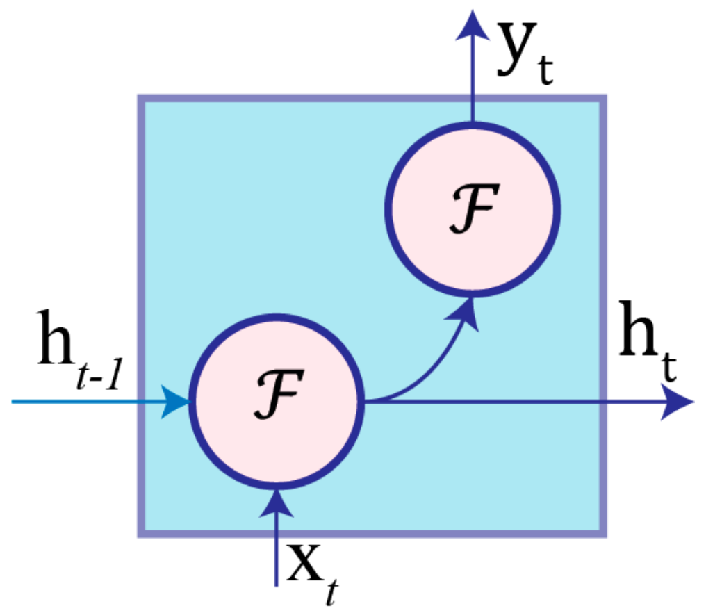
3.1. Recurrent Neural Networks
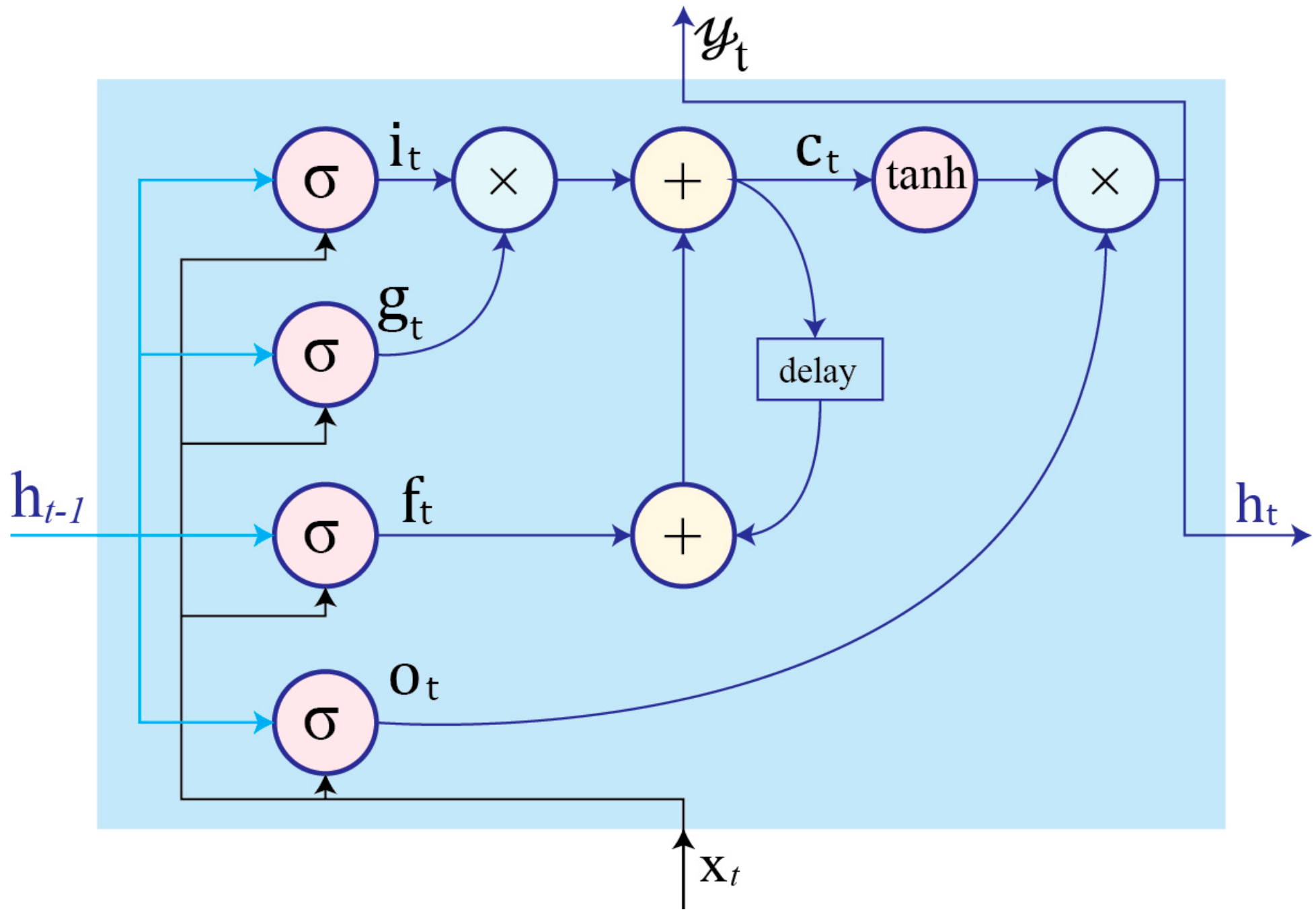
3.2. Long Short-Term Memory (LSTM)
- Input gate controls the flow of new information to the cell.
- Forget gate determins when to forget content regarding the internal state.
- Output gate controls which information flows to the output.
- Input modulation gate is the main input to the cell.
- Internal state handles cell internal recurrence.
- Hidden state contains information from previously seen samples within the context window:
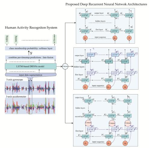
4. Proposed DRNN Architectures
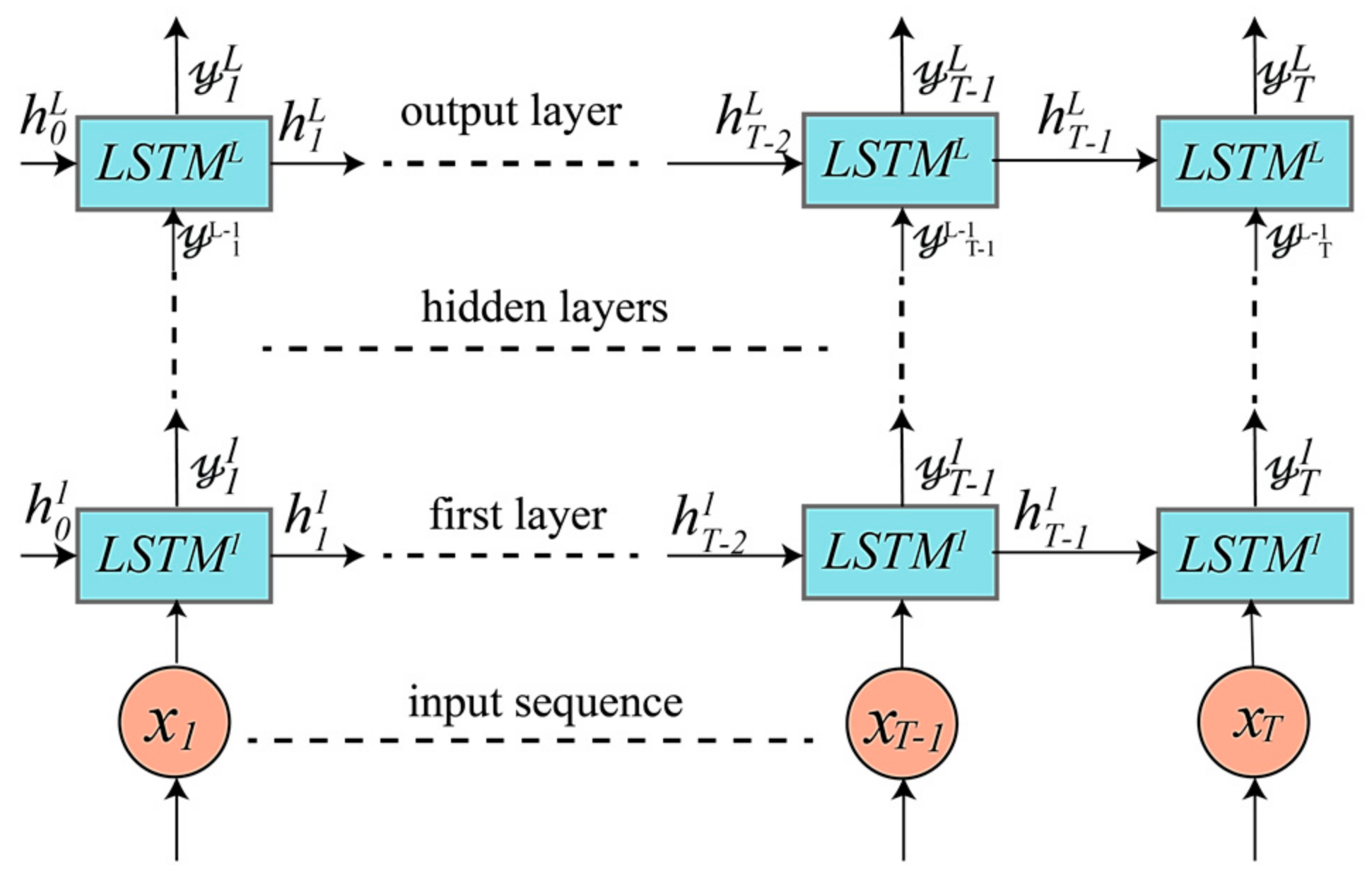
4.1. Unidirectional LSTM-Based DRNNs Model
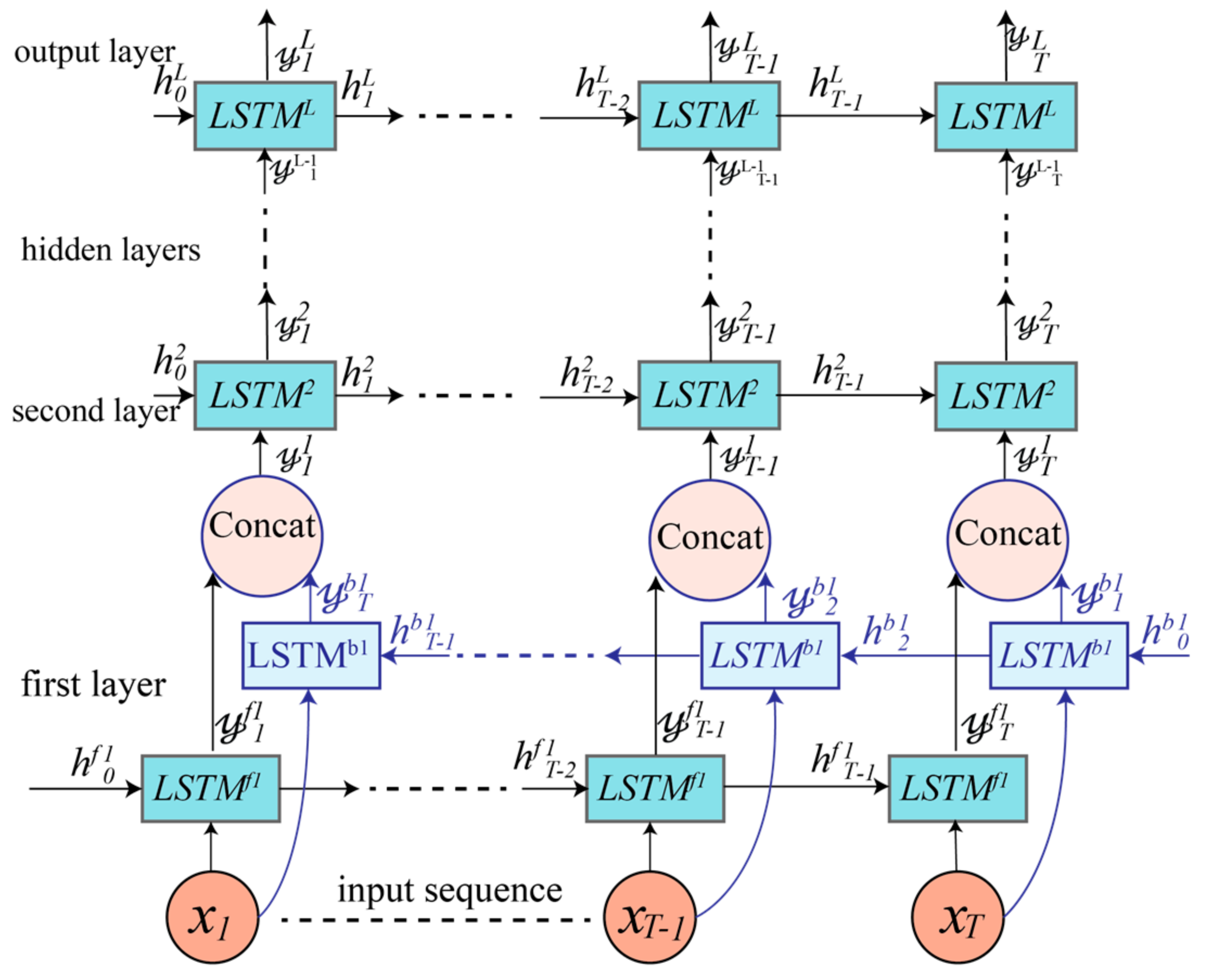
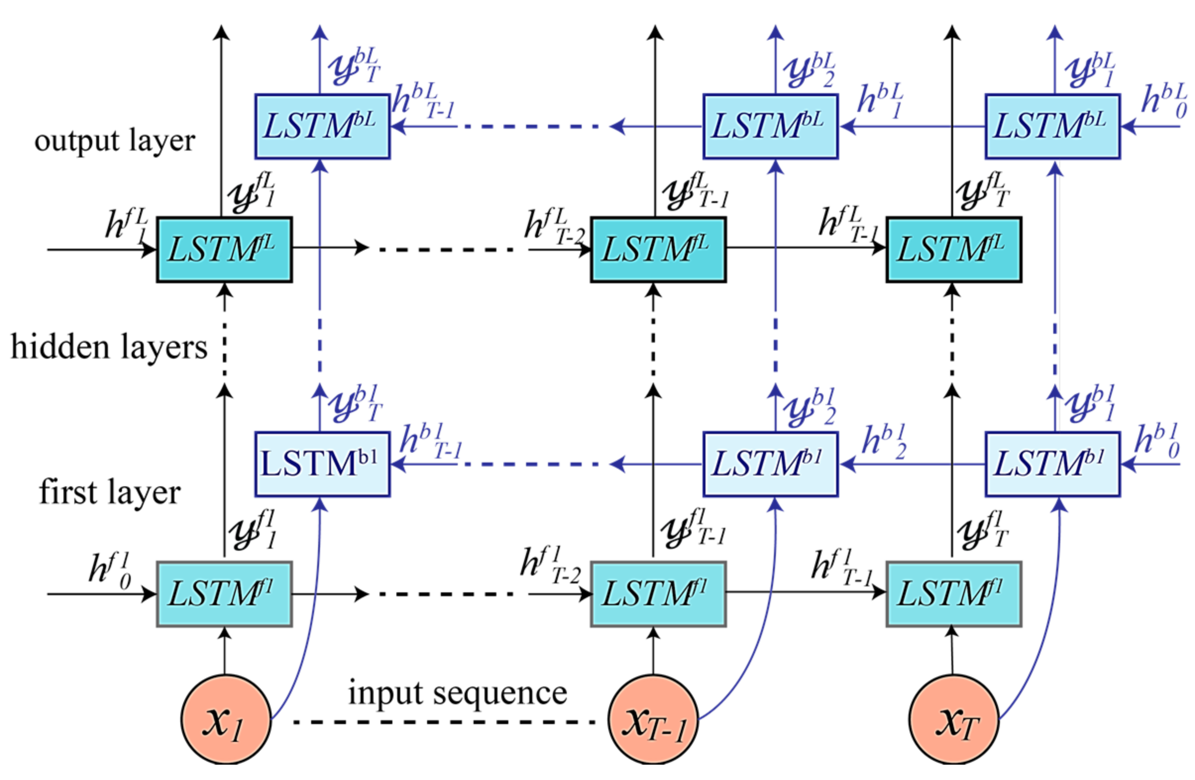
4.2. Bidirectional LSTM-Based DRNN Model
4.3. Cascaded Bidirectional and Unidirectional LSTM-based DRNN Model
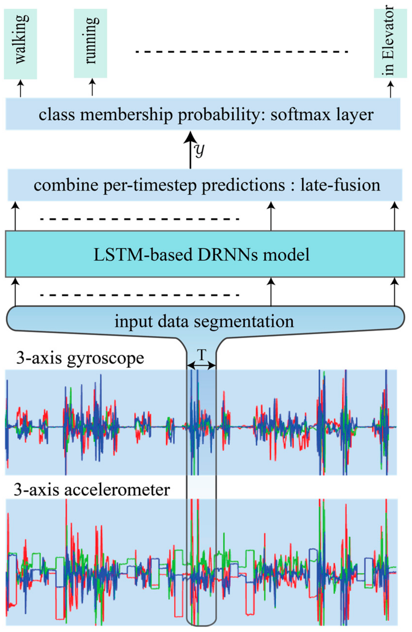
5. Experimental Setup
5.1. Datasets of Human Activities
- 1)
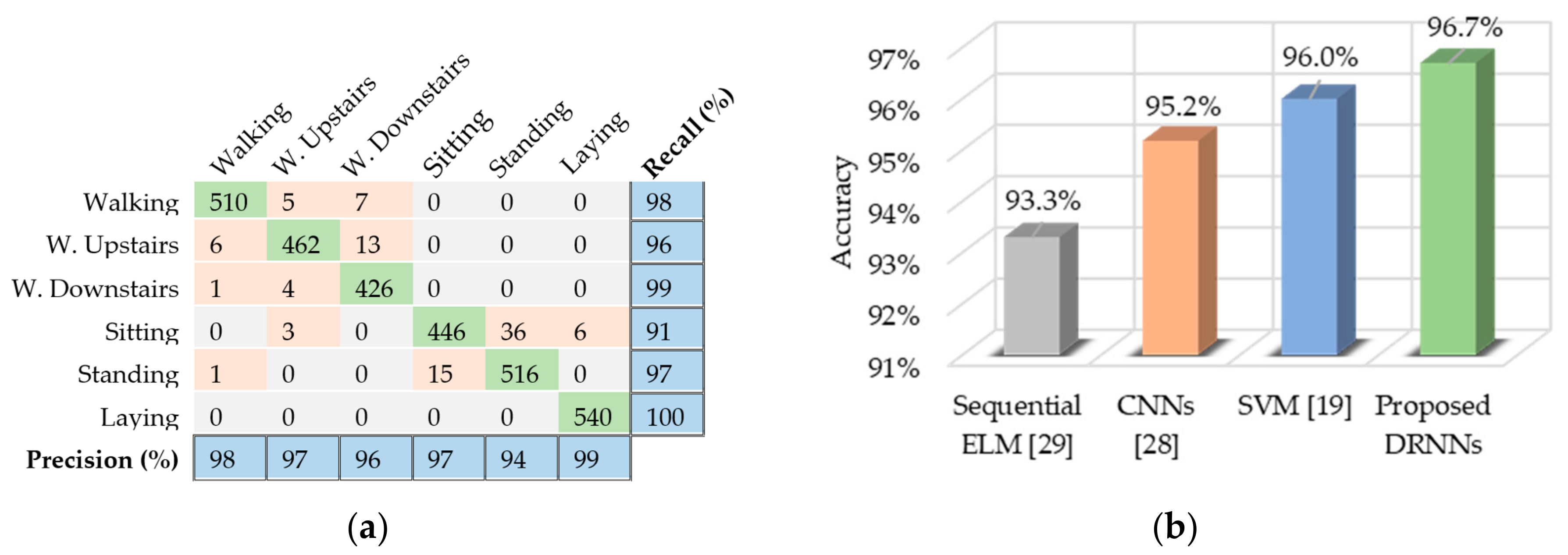
- UCI-HAD [19]: Dataset for activities of daily living (ADL) recorded by using a waist-mounted smartphone with an embedded 3-axis accelerometer, gyroscope, and magnetometer. All nine channels from the 3-axis sensors are used as inputs for our DRNN model at every time step. This dataset contains only six classes: walking, ascending stairs, descending stairs, sitting, standing, and laying.
- 2)
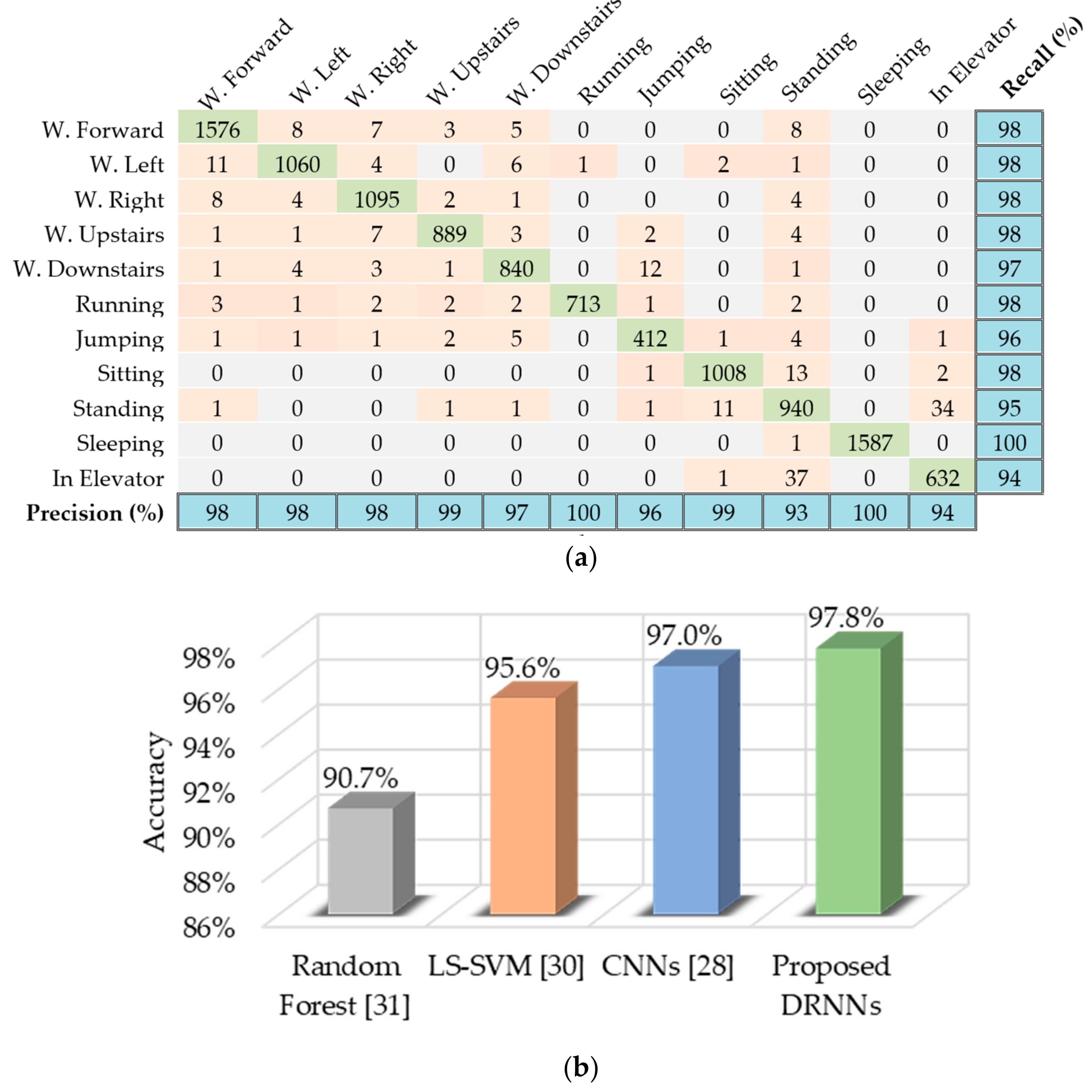
- USC-HAD [20]: Dataset collected by using a high performance IMU (3D accelerometer and gyroscope) sensor positioned on volunteers’ front right hips. The dataset contains 12 basic human activities: walking forward, walking left, walking right, walking upstairs, walking downstairs, running forward, jumping up, sitting, standing, sleeping, in elevator up, and in elevator down. We considered 11 classes by combining the last two activities into a single “in elevator” activity. The reason for this combination is that the model is unable to differentiate between the two classes using only a single IMU sensor. Additional barometer readings are required to determine height changes in an elevator and discriminate between the two classes (up or down in elevator).
- 3)
- Opportunity [21]: Dataset comprised of ADL recorded in a sensor-rich environment. We consider only recordings from on-body sensors, which are seven IMUs and 12 3D-accelerometers placed on various body parts. There are 18 activity classes: opening and closing two types of doors, opening and closing three drawers at different heights, opening and closing a fridge, opening and closing a dishwasher, cleaning a table, drinking from a cup, toggling a switch, and a null-class for any non-relevant actions.
- 4)
- Daphnet FOG [22]: Dataset containing movement data from patients with Parkinson’s disease (PD) who suffer from freezing of gait (FOG) symptoms. The dataset was built using three 3D-accelerometers attached to the shank, thigh, and lower back of the patients. Two classes (freeze and normal) were considered depending on whether or not the gait of a patient was frozen when the sample was recorded. We used this dataset to train our model to detect FOG episodes in PD patients and prove the suitability of our model for gait analysis using only wearable sensors.
- 5)
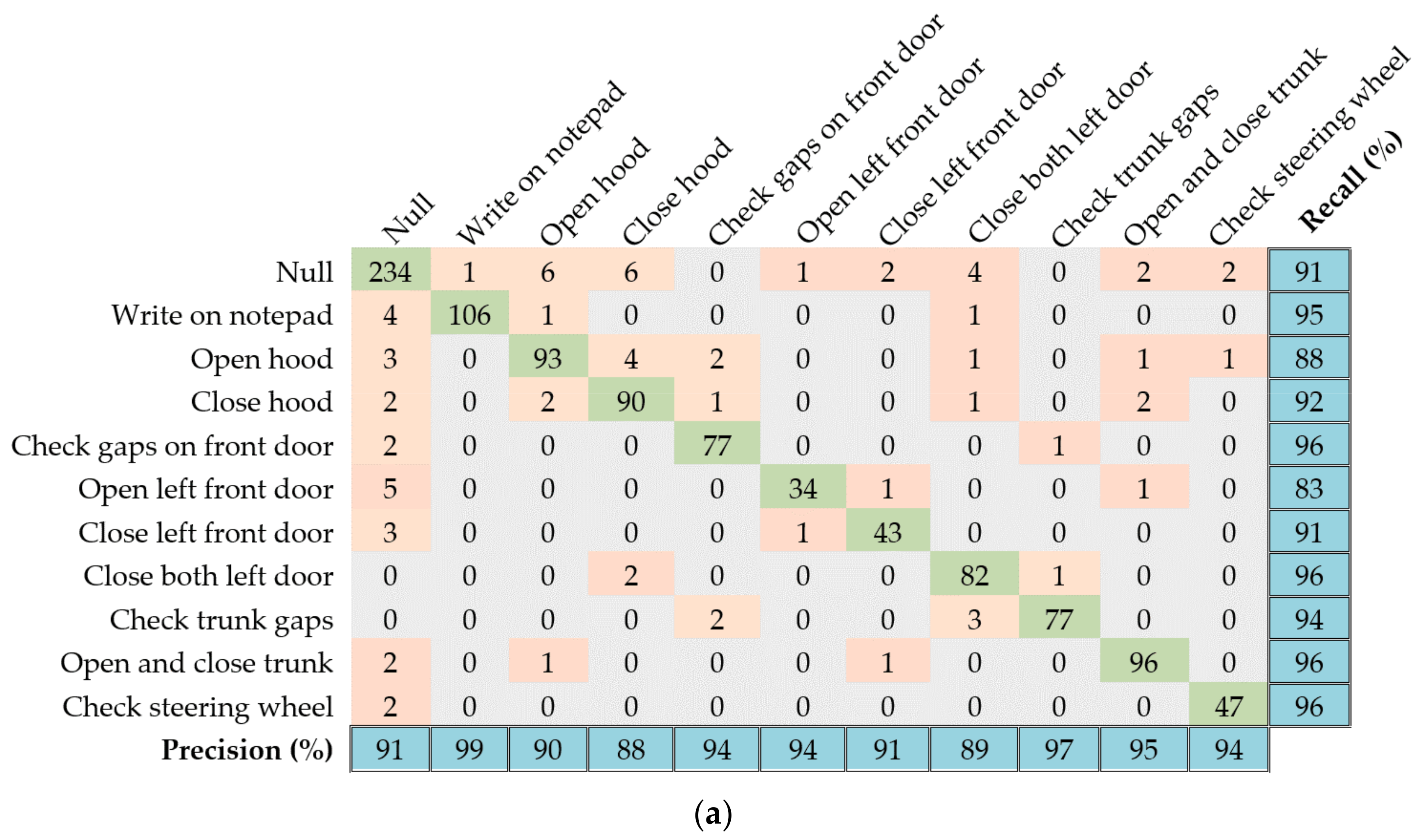
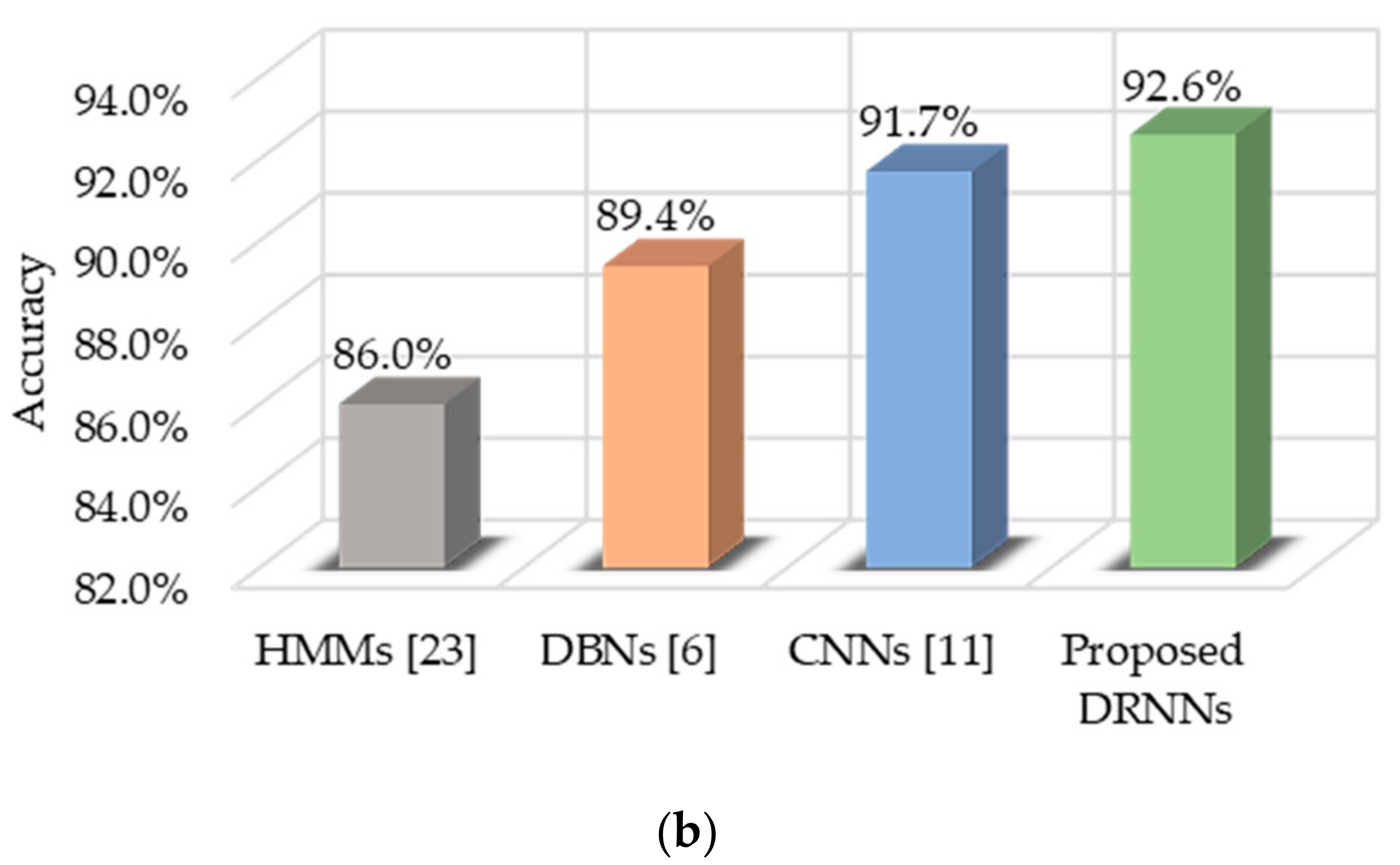
- Skoda [23]: Dataset containing activities of an employee in a car maintenance scenario. We consider recordings from a single 3D accelerometer, which is placed on the right hand of an employee. The dataset contains 11 activity classes: writing on a notepad, opening hood, closing hood, checking gaps on front door, opening left front door, closing left front door, closing both left doors, checking trunk gaps, opening and closing trunk, and a null-class for any non-relevant actions.
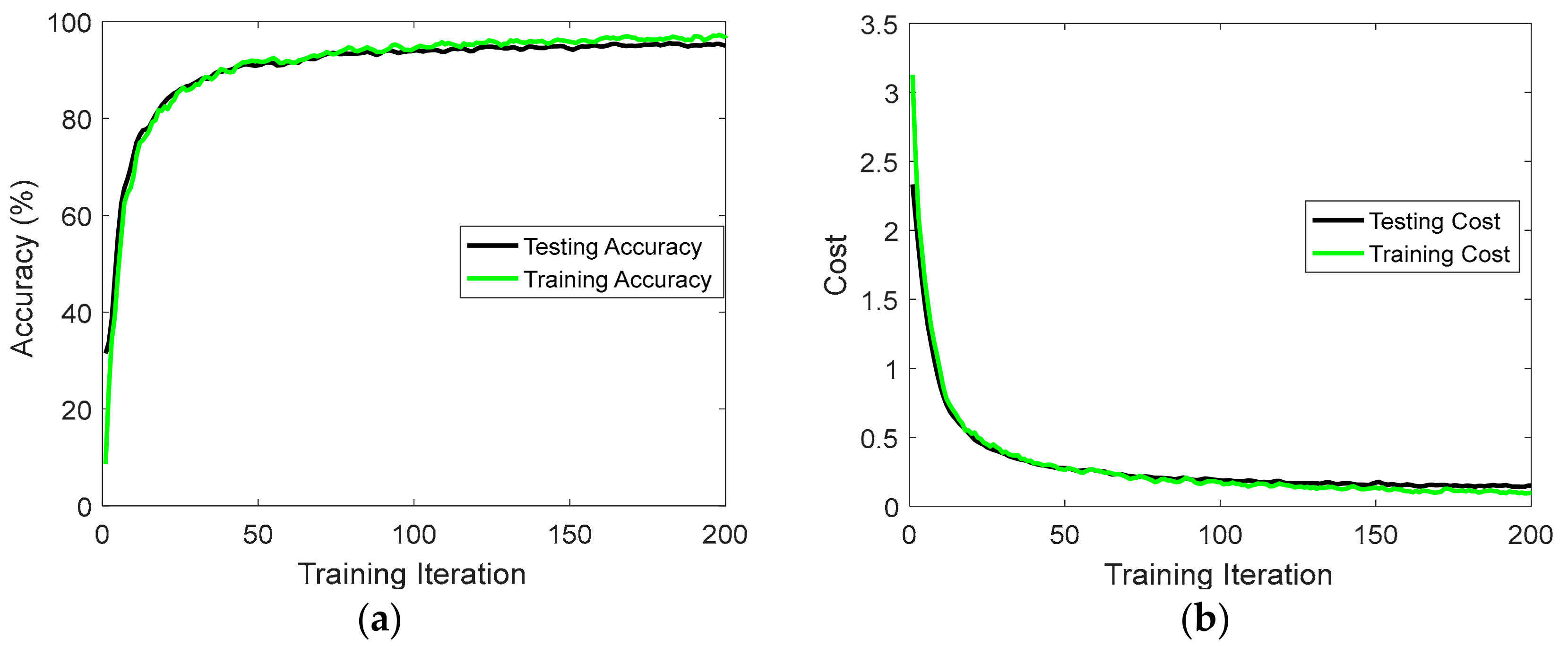
5.2. Training
5.3. Performance Metrics
- 1)
- Precision: Measures the number of true samples out of those classified as positive. The overall precision is the average of the precisions for each class:where is the true positive rate of a class , is the false positive rate, and is the number of classes in the dataset.
- 2)
- Recall (Sensitivity): Measures the number correctly classified samples out of the total samples of a class. The overall recall is the average of the recalls for each class:where is the false negative rate of a class .
- 3)
- Accuracy: Measures the proportion of correctly predicted labels over all predictions:where is the overall true positive rate for a classifier on all classes, is the overall true negative rate, is the overall false positive rate, and is the overall false negative rate.
- 4)
- F1-score: A weighted harmonic mean of precision and recall:where is the number of samples of a class and is the total number of samples in a set with classes. The F1-score is typically adopted for imbalanced datasets that have more samples of one class and less of another, such as the Daphnet FOG dataset. There are more instances of normal walking (majority class) than of FOG (minority class). The Opportunity dataset is also imbalanced because there are many more instances of the null class than any of the other classes. Using accuracy as a performance metric in imbalanced datasets can be misleading, because any classifier can perform well by correctly classifying the majority class even if it wrongly classifies the minority class.
6. Results
6.1. UCI-HAD
6.2. USC-HAD
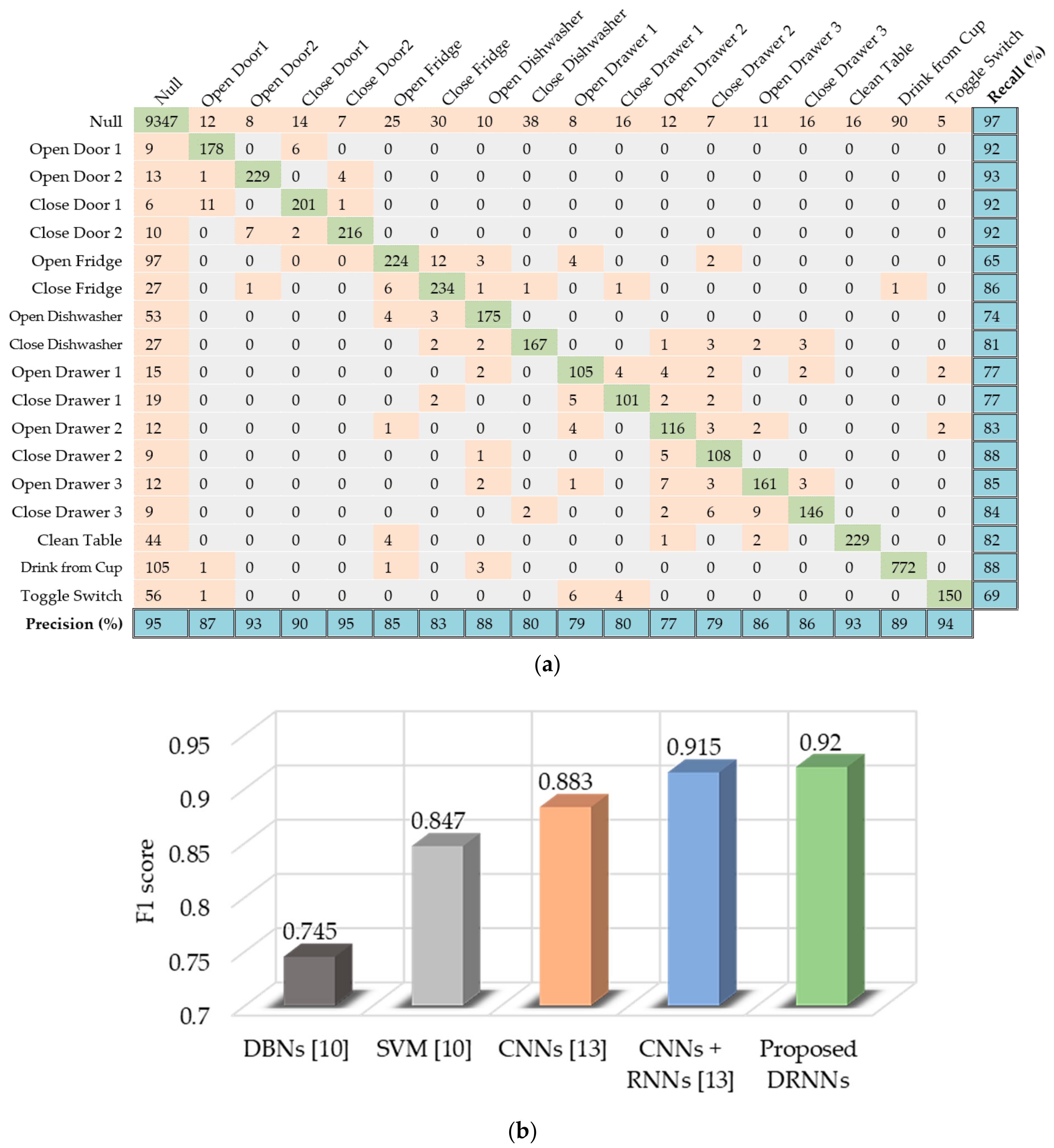
6.3. Opportunity
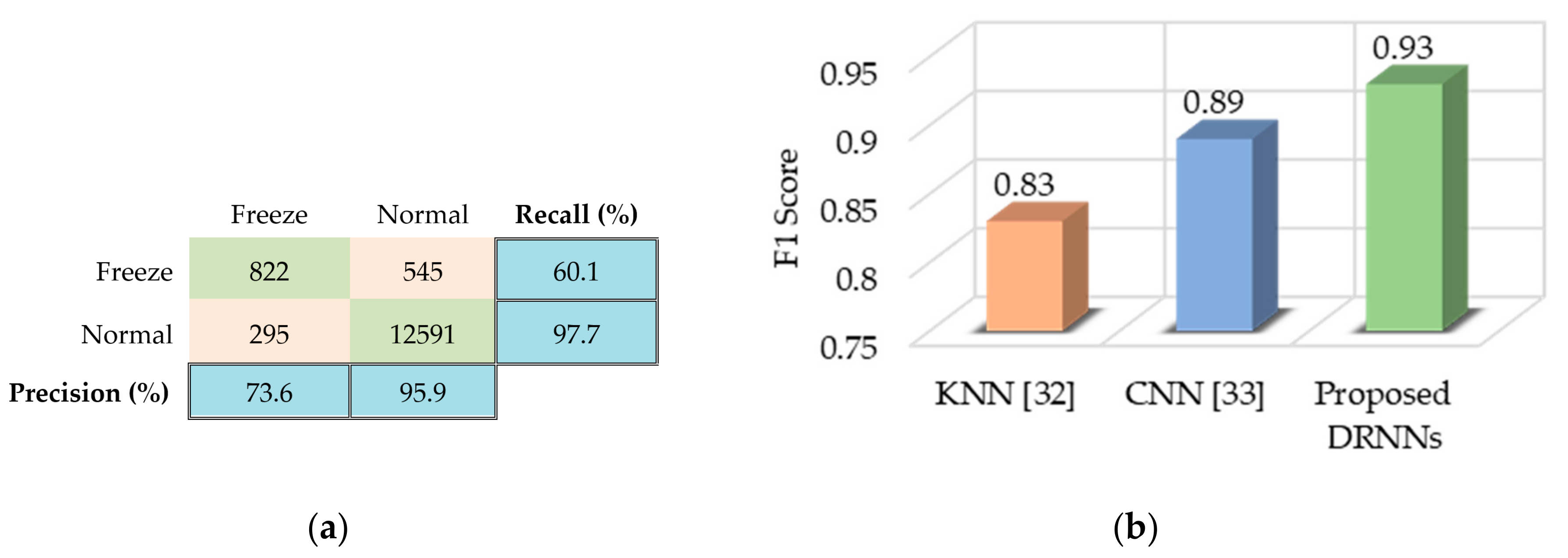
6.4. Daphnet FOG
6.5. Skoda
7. Discussion
8. Conclusions
Author Contributions
Conflicts of Interest
References
- Graves, A.; Mohamed, A.; Hinton, G. Speech recognition with deep recurrent neural networks. In Proceedings of the IEEE International Conference on Acoustics, Speech and Signal Processing, Vancouver, BC, Canada, 26–31 May 2013; pp. 6645–6649. [Google Scholar]
- Sundermeyer, M.; Schlüter, R.; Ney, H. LSTM Neural Networks for Language Modeling. In Proceedings of the Thirteenth Annual Conference of the International Speech Communication Association, Portland, OR, USA, 9–13 September 2012. [Google Scholar]
- Yao, L.; Cho, K.; Ballas, N.; Paí, C.; Courville, A. Describing Videos by Exploiting Temporal Structure. In Proceedings of the IEEE International Conference on Computer Vision, Santiago, Chile, 7–13 December 2015. [Google Scholar]
- Graves, A. Supervised Sequence Labelling with Recurrent Neural Networks; Studies in Computational Intelligence; Springer: Berlin/Heidelberg, Germany, 2012; Volume 385, ISBN 978-3-642-24796-5. [Google Scholar]
- Plötz, T.; Hammerla, N.Y.; Olivier, P. Feature Learning for Activity Recognition in Ubiquitous Computing. In Proceedings of the Twenty-Second International Joint Conference on Artificial Intelligence, Barcelona, Catalonia, Spain, 16–22 July 2011; Volume 2, pp. 1729–1734. [Google Scholar]
- Alsheikh, M.A.; Selim, A.; Niyato, D.; Doyle, L.; Lin, S.; Tan, H.-P. Deep Activity Recognition Models with Triaxial Accelerometers. In Proceedings of the AAAI Workshop: Artificial Intelligence Applied to Assistive Technologies and Smart Environments, Phoenix, AZ, USA, 12 February 2016. [Google Scholar]
- Zeng, M.; Nguyen, L.T.; Yu, B.; Mengshoel, O.J.; Zhu, J.; Wu, P.; Zhang, J. Convolutional Neural Networks for Human Activity Recognition using Mobile Sensors. In Proceedings of the 6th International Conference on Mobile Computing, Applications and Services, Austin, TX, USA, 6–7 November 2014; pp. 197–205. [Google Scholar]
- Chen, Y.; Xue, Y. A Deep Learning Approach to Human Activity Recognition Based on Single Accelerometer. In Proceedings of the IEEE International Conference on Systems, Man, and Cybernetics, Hong Kong, China, 20 June 2015; pp. 1488–1492. [Google Scholar]
- Hessen, H.-O.; Tessem, A.J. Human Activity Recognition with Two Body-Worn Accelerometer Sensors. Master’s Thesis, Norwegian University of Science and Technology, Trondheim, Norway, 2015. [Google Scholar]
- Yang, J.B.; Nguyen, M.N.; San, P.P.; Li, X.L.; Krishnaswamy, S. Deep convolutional neural networks on multichannel time series for human activity recognition. In Proceedings of the 24th International Joint Conference on Artificial Intelligence (IJCAI), Buenos Aires, Argentina, 25–31 July 2015. [Google Scholar]
- Ravi, D.; Wong, C.; Lo, B.; Yang, G.-Z. Deep learning for human activity recognition: A resource efficient implementation on low-power devices. In Proceedings of the IEEE 13th International Conference on Wearable and Implantable Body Sensor Networks (BSN), San Francisco, CA, USA, 14–17 June 2016; pp. 71–76. [Google Scholar]
- Waibel, A.; Hanazawa, T.; Hinton, G.; Shikano, K.; Lang, K.J. Phoneme recognition using time-delay neural networks. IEEE Trans. Acoust. Speech Signal Process. 1989, 37, 328–339. [Google Scholar] [CrossRef]
- Ordóñez, F.J.; Roggen, D. Deep convolutional and LSTM recurrent neural networks for multimodal wearable activity recognition. Sensors 2016, 16, 115. [Google Scholar] [CrossRef] [PubMed]
- Fan, Y.; Qian, Y.; Xie, F.; Soong, F.K. TTS synthesis with bidirectional LSTM based Recurrent Neural Networks. In Proceedings of the Fifteenth Annual Conference of the International Speech Communication Association, Singapore, 14–18 September 2014; pp. 1964–1968. [Google Scholar]
- Hochreiter, S.; Bengio, Y.; Frasconi, P.; Schmidhuber, J. Gradient Flow in Recurrent Nets: The Difficulty of Learning Long-Term Dependencies. In Field Guide to Dynamical Recurrent Networks; Kremer, S., Kolen, J., Eds.; Wiley-IEEE Press: Hoboken, NJ, USA, 2001; pp. 237–243. ISBN 9780470544037. [Google Scholar]
- Kittler, J.; Hater, M.; Duin, R.P.W. Combining classifiers. IEEE Trans. Pattern Anal. Mach. Intell. 1996, 2, 226–239. [Google Scholar] [CrossRef]
- Schuster, M.; Paliwal, K.K. Bidirectional recurrent neural networks. IEEE Trans. Signal Process. 1997, 45, 2673–2681. [Google Scholar] [CrossRef]
- Wu, Y.; Schuster, M.; Chen, Z.; Le, Q.V.; Norouzi, M.; Macherey, W.; Krikun, M.; Cao, Y.; Gao, Q.; Macherey, K.; et al. Google’s Neural Machine Translation System: Bridging the Gap between Human and Machine Translation. CoRR 2016, arXiv:arXiv:1609.08144. [Google Scholar]
- Anguita, D.; Ghio, A.; Oneto, L.; Parra, X.; Reyes-Ortiz, J.L. A Public Domain Dataset for Human Activity Recognition Using Smartphones. In Proceedings of the European Symposium on Artificial Neural Networks, Bruges, Belgium, 24–26 April 2013; pp. 24–26. [Google Scholar]
- Zhang, M.; Sawchuk, A.A. USC-HAD: A Daily Activity Dataset for Ubiquitous Activity Recognition Using Wearable Sensors. In Proceedings of the 2012 ACM Conference on Ubiquitous Computing, Pittsburgh, PA, USA, 5–8 September 2012; pp. 1036–1043. [Google Scholar]
- Chavarriaga, R.; Sagha, H.; Calatroni, A.; Digumarti, S.T.; Tröster, G.; Millán, J.D.R.; Roggen, D. The Opportunity challenge: A benchmark database for on-body sensor-based activity recognition. Pattern Recognit. Lett. 2013, 34, 2033–2042. [Google Scholar] [CrossRef]
- Bachlin, M.; Plotnik, M.; Roggen, D.; Maidan, I.; Hausdorff, J.M.; Giladi, N.; Troster, G. Wearable assistant for Parkinson’s disease patients with the freezing of gait symptom. IEEE Trans. Inf. Technol. Biomed. 2010, 14, 436–446. [Google Scholar] [CrossRef] [PubMed]
- Zappi, P.; Lombriser, C.; Stiefmeier, T.; Farella, E.; Roggen, D.; Benini, L.; Tröster, G. Activity Recognition from On-Body Sensors: Accuracy-Power Trade-Off by Dynamic Sensor Selection. In Wireless Sensor Networks; Springer: Berlin/Heidelberg, Germany, 2008; pp. 17–33. [Google Scholar]
- Goodfellow, I.; Bengio, Y.; Courville, A. Optimization for Training Deep Models. In Deep Learning; The MIT Press: Cambridge, MA, USA, 2016; p. 800. ISBN 978-0262035613. [Google Scholar]
- Abadi, M.; Agarwal, A.; Barham, P.; Brevdo, E.; Chen, Z.; Citro, C.; Corrado, G.S.; Davis, A.; Dean, J.; Devin, M.; et al. TensorFlow: Large-Scale Machine Learning on Heterogeneous Distributed Systems. 2015. Available online: https://www.tensorflow.org/ (accessed on 13 September 2017).
- Pham, V.; Bluche, T.; Kermorvant, C.; Louradour, J. Dropout Improves Recurrent Neural Networks for Handwriting Recognition. In Proceedings of the 14th International Conference on Frontiers in Handwriting Recognition, Crete, Greece, 1–4 September 2014; pp. 285–290. [Google Scholar]
- Sokolova, M.; Lapalme, G. A systematic analysis of performance measures for classification tasks. Inf. Process. Manag. 2009, 45, 427–437. [Google Scholar] [CrossRef]
- Jiang, W. Human Activity Recognition using Wearable Sensors by Deep Convolutional Neural Networks. In Proceedings of the 23rd ACM International Conference on Multimedia, Brisbane, Australia, 26–30 October 2015; pp. 1307–1310. [Google Scholar]
- Chandan Kumar, R.; Bharadwaj, S.S.; Sumukha, B.N.; George, K. Human activity recognition in cognitive environments using sequential ELM. In Proceedings of the Second International Conference on Cognitive Computing and Information Processing, Mysuru, India, 12–13 August 2016; pp. 1–6. [Google Scholar]
- Zheng, Y. Yuhuang Human Activity Recognition Based on the Hierarchical Feature Selection and Classification Framework. J. Electr. Comput. Eng. 2015, 2015, 34. [Google Scholar] [CrossRef]
- Prakash Reddy Vaka, B.B. A Pervasive Middleware for Activity Recognition with Smartphones. Master’s Thesis, University of Missouri, Columbia, MO, USA, 2015. [Google Scholar]
- Hammerla, N.; Kirkham, R. On Preserving Statistical Characteristics of Accelerometry Data using their Empirical Cumulative Distribution. In Proceedings of the 2013 International Symposium on Wearable Computers, Zurich, Switzerland, 9–12 September 2013; pp. 65–68. [Google Scholar]
- Ravi, D.; Wong, C.; Lo, B.; Yang, G.-Z. A deep learning approach to on-node sensor data analytics for mobile or wearable devices. IEEE J. Biomed. Health Inform. 2017, 21, 56–64. [Google Scholar] [CrossRef] [PubMed]


| Dataset | # of Classes | Sensors | # of Subjects | Sampling Rate | Training Window Length | # of Training Examples | # of Testing Examples |
|---|---|---|---|---|---|---|---|
| UCI-HAD [19] | 6 | 3D Acc., Gyro., and Magn. of a smartphone | 30 | 50 Hz | 128 | 11,988 | 2997 |
| USC-HAD [20] | 12 | 3D Acc. & Gyro | 14 (5 sessions) | 100 Hz | 128 | 44,000 | 11,000 |
| Opportunity [21] | 18 | 7 IMU sensors (3D ACC, Gyro & Mag.) & 12 Acc. | 4 (5 sessions) | 30 Hz | 24 | 55,576 | 13,894 |
| Daphnet FOG [22] | 2 | 3 3D Acc. | 10 | 64 Hz | 32 | 57,012 | 14,253 |
| Skoda [23] | 11 | 3D Acc. | 1 (19 sessions) | 98 Hz | 128 | 4411 | 1102 |
| Model | Dataset | Overall Accuracy | Average Precision | Average Recall | F1 Score |
|---|---|---|---|---|---|
| Unidirectional DRNN | UCI | 96.7% | 96.8% | 96.7% | 0.96 |
| Unidirectional DRNN | USC-HAD | 97.8% | 97.4.0% | 97.4% | 0.97 |
| Bidirectional DRNN | Opportunity | 92.5% | 86.7% | 83.5% | 0.92 |
| Cascaded DRNN | Daphnet FOG | 94.1% | 84.7% | 78.9% | 0.93 |
| Cascaded DRNN | Skoda | 92.6% | 93.0% | 92.6% | 0.92 |
© 2017 by the authors. Licensee MDPI, Basel, Switzerland. This article is an open access article distributed under the terms and conditions of the Creative Commons Attribution (CC BY) license (http://creativecommons.org/licenses/by/4.0/).
Share and Cite
Murad, A.; Pyun, J.-Y. Deep Recurrent Neural Networks for Human Activity Recognition. Sensors 2017, 17, 2556. https://doi.org/10.3390/s17112556
Murad A, Pyun J-Y. Deep Recurrent Neural Networks for Human Activity Recognition. Sensors. 2017; 17(11):2556. https://doi.org/10.3390/s17112556
Chicago/Turabian StyleMurad, Abdulmajid, and Jae-Young Pyun. 2017. "Deep Recurrent Neural Networks for Human Activity Recognition" Sensors 17, no. 11: 2556. https://doi.org/10.3390/s17112556
APA StyleMurad, A., & Pyun, J.-Y. (2017). Deep Recurrent Neural Networks for Human Activity Recognition. Sensors, 17(11), 2556. https://doi.org/10.3390/s17112556