
Enhance the Quality of Crowdsensing for Fine-Grained Urban Environment Monitoring via Data Correlation

Abstract
:1. Introduction
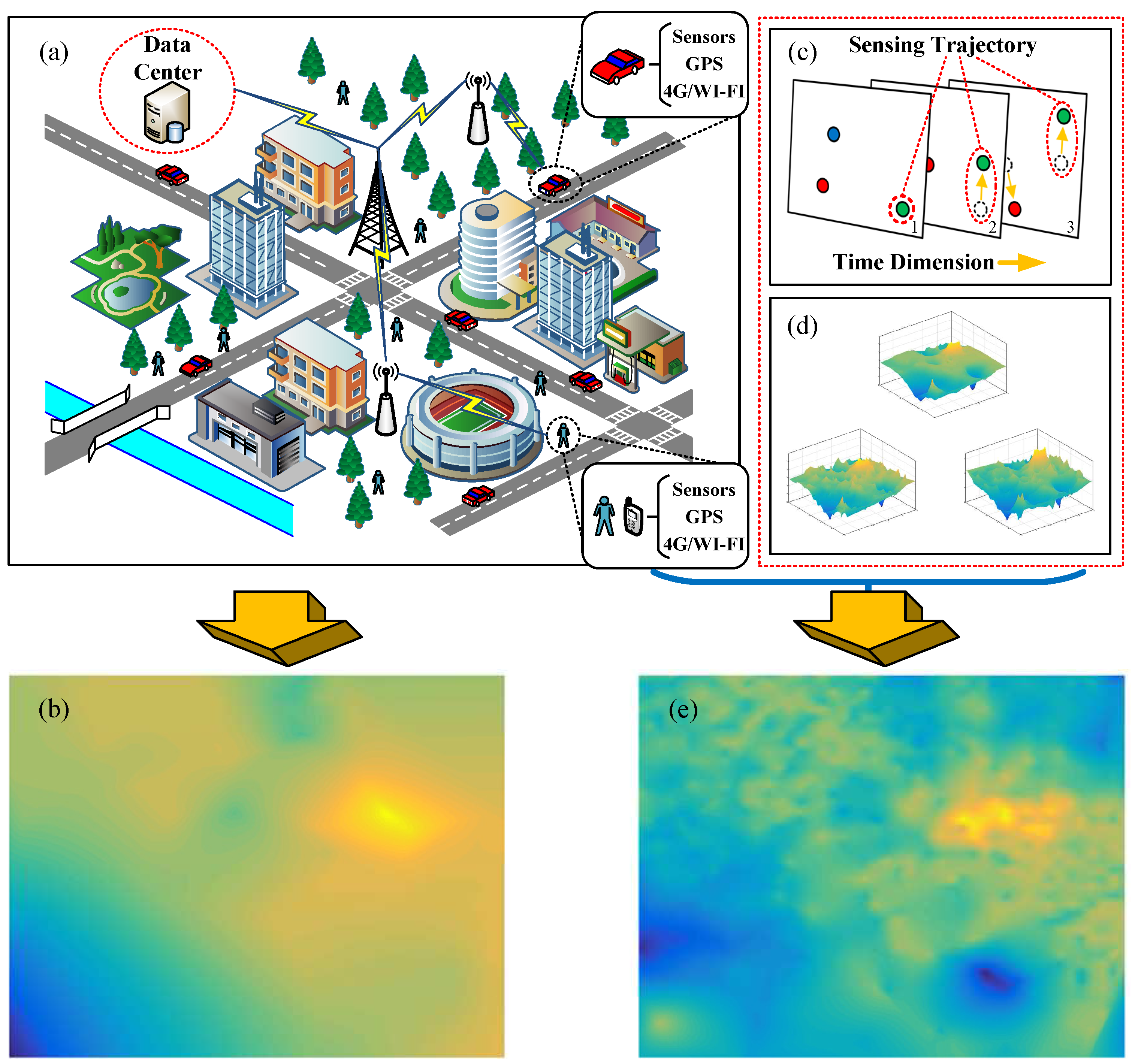
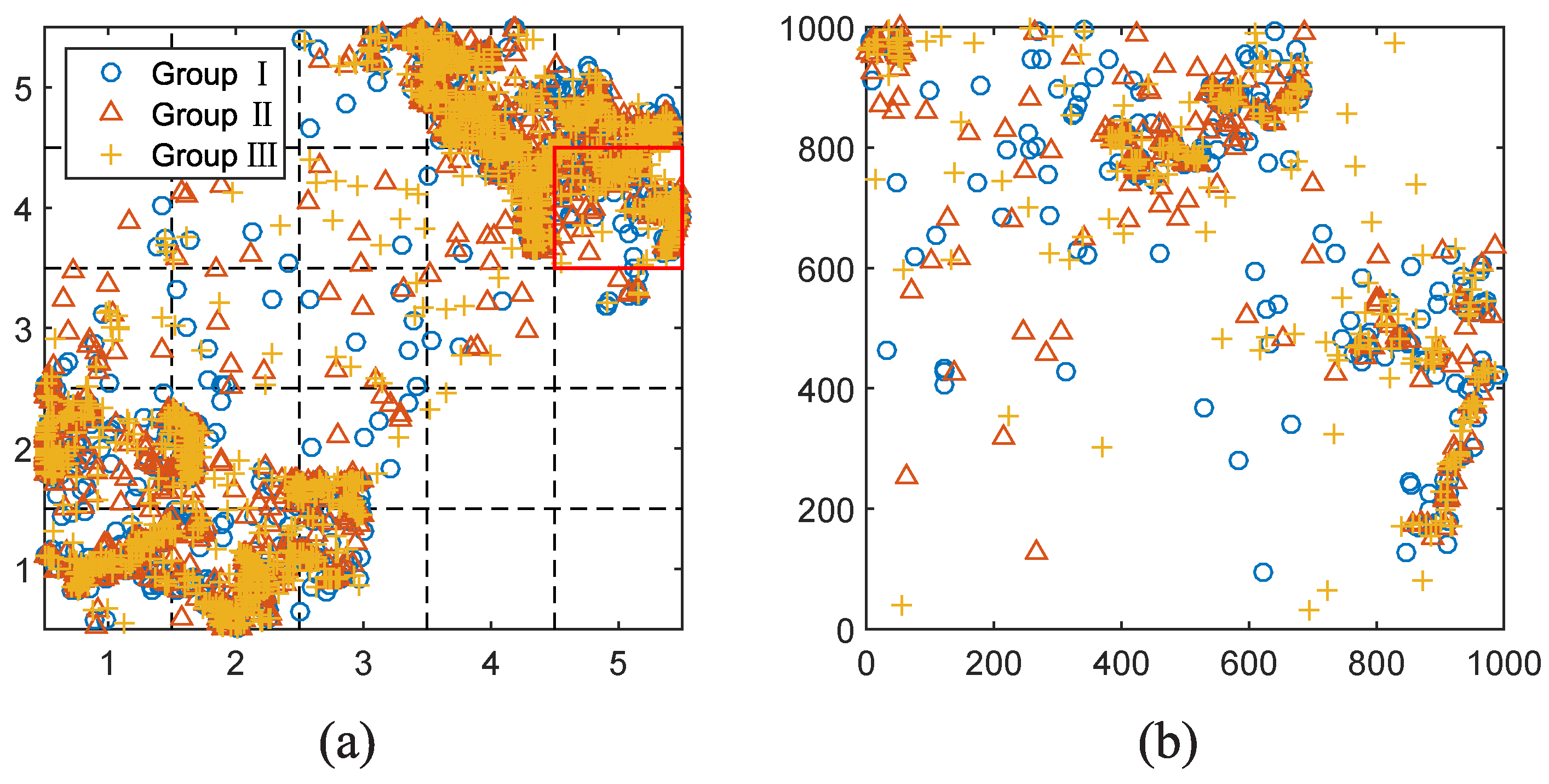
- Temporal correlation of sensory data. Researchers of [17] revealed the pervasive existence of time stability feature among environmental phenomenons, such as temperature, humidity and light. This feature indicates that most environmental phenomenons will not change dramatically and maintain stable for a while. On the other hand, the frequency of participants sending their measurements is much higher than that of environment changing. Utilizing temporal correlation is to leverage measurement data in a correlated time period rather than a moment. Due to the dynamic feature of crowdsensing participants, a discrete participant at a moment is converted into a sensing trajectory in correlated time period (see Figure 1c), which could decrease the area of blank zones.
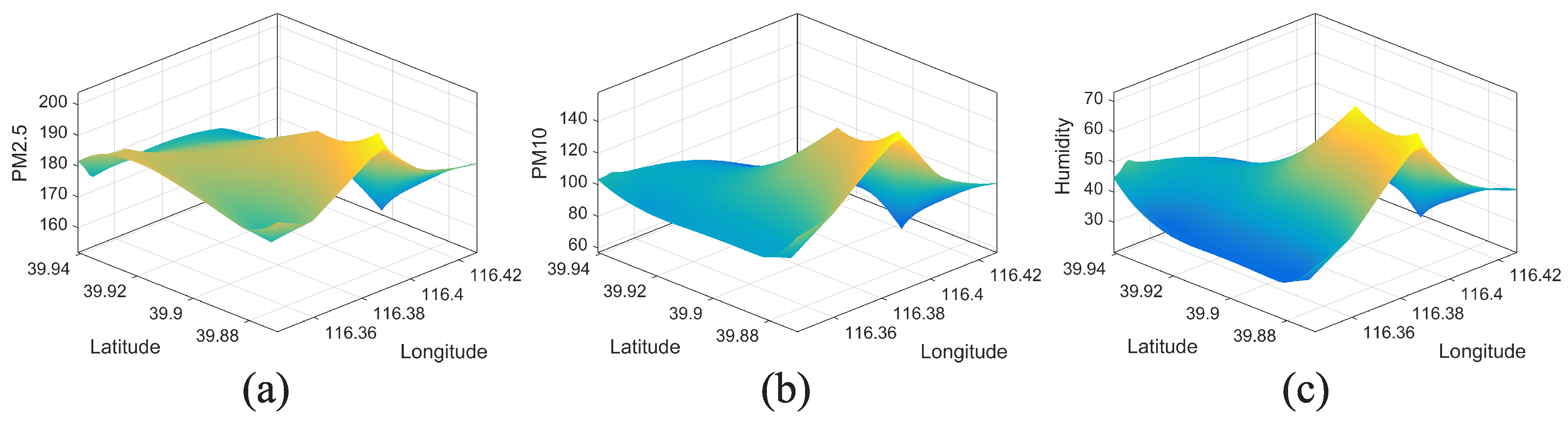
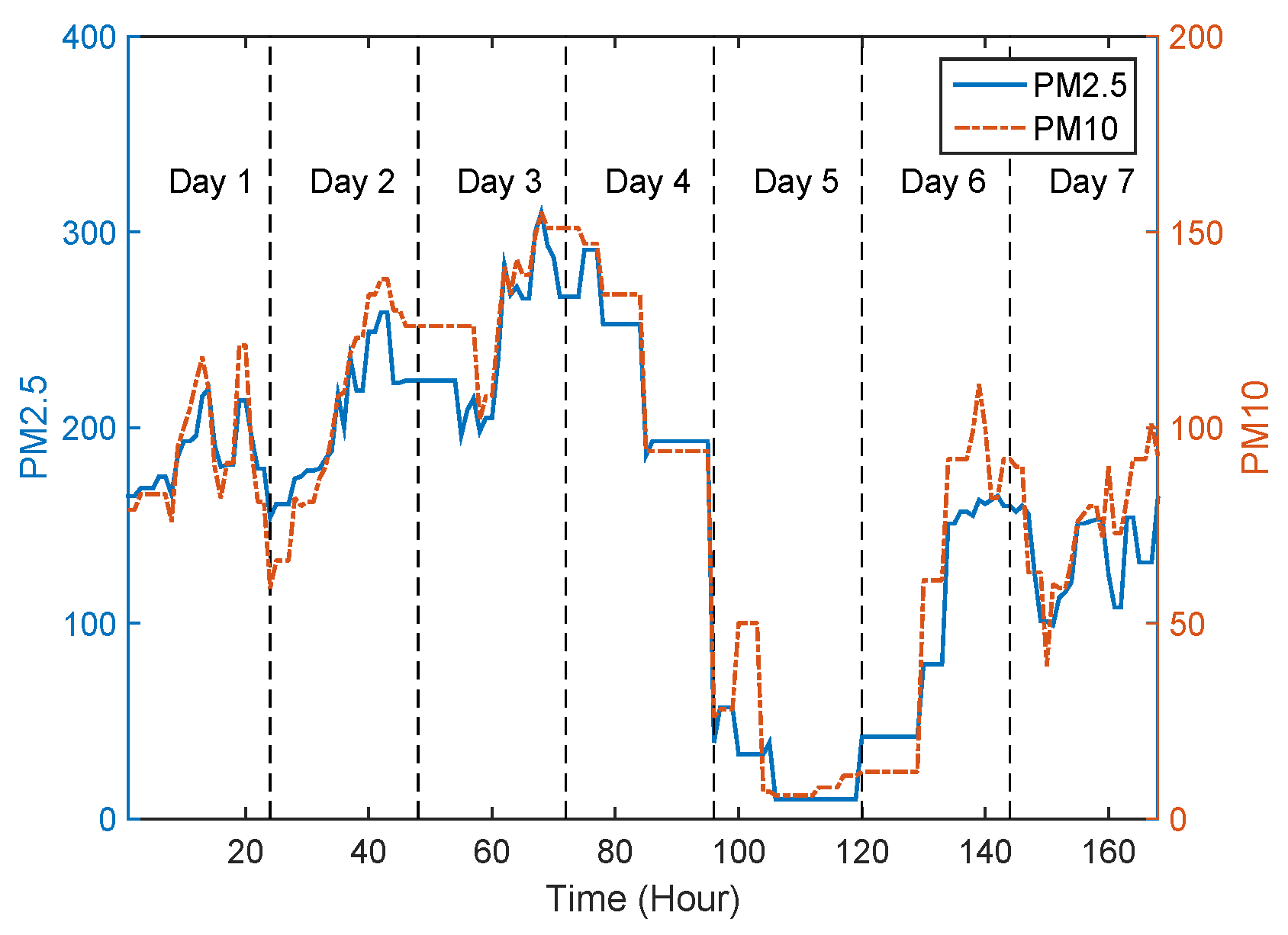
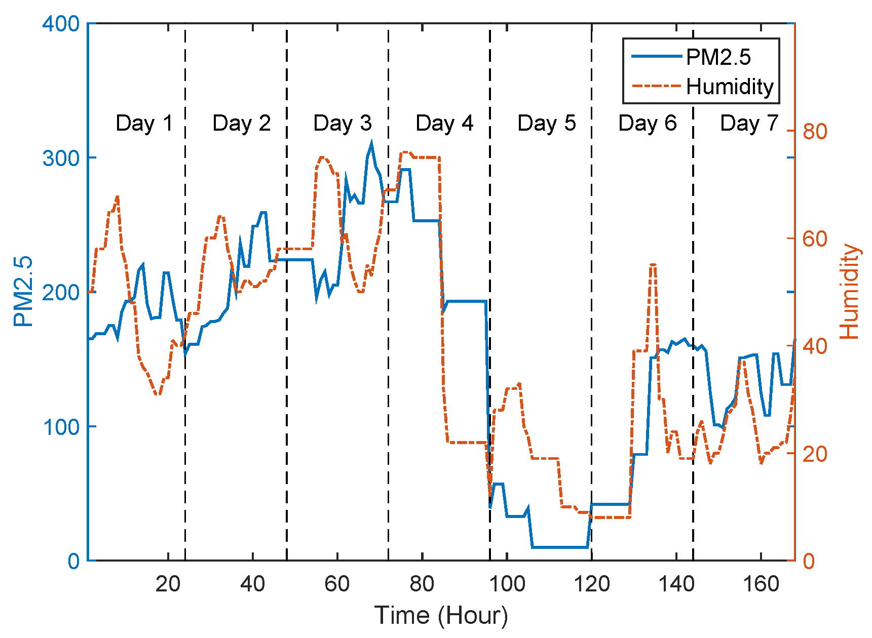
- Category correlation of sensory data. Many existing researches [20,21,22] show the strong correlation among some categories of sensory data (see Figure 1d). Taking air quality data for example, three mainly concerned atmospheric pollutants, the concentration of PM, PM10, and NO, have clear correlation. Therefore, if there exist some correlated sensory data in blank zones, then the correlated information is able to recover the target environmental phenomenon.
2. Urban Monitoring via Crowdsensing and Sensing Restriction of Crowdsensing
2.1. Generation of Sensing Image via Crowdsensing Network
- There is only one crowdsensing node in . For this case, the corresponding entry in matrix is equal to the sensory data provided by the only crowdsensing node.
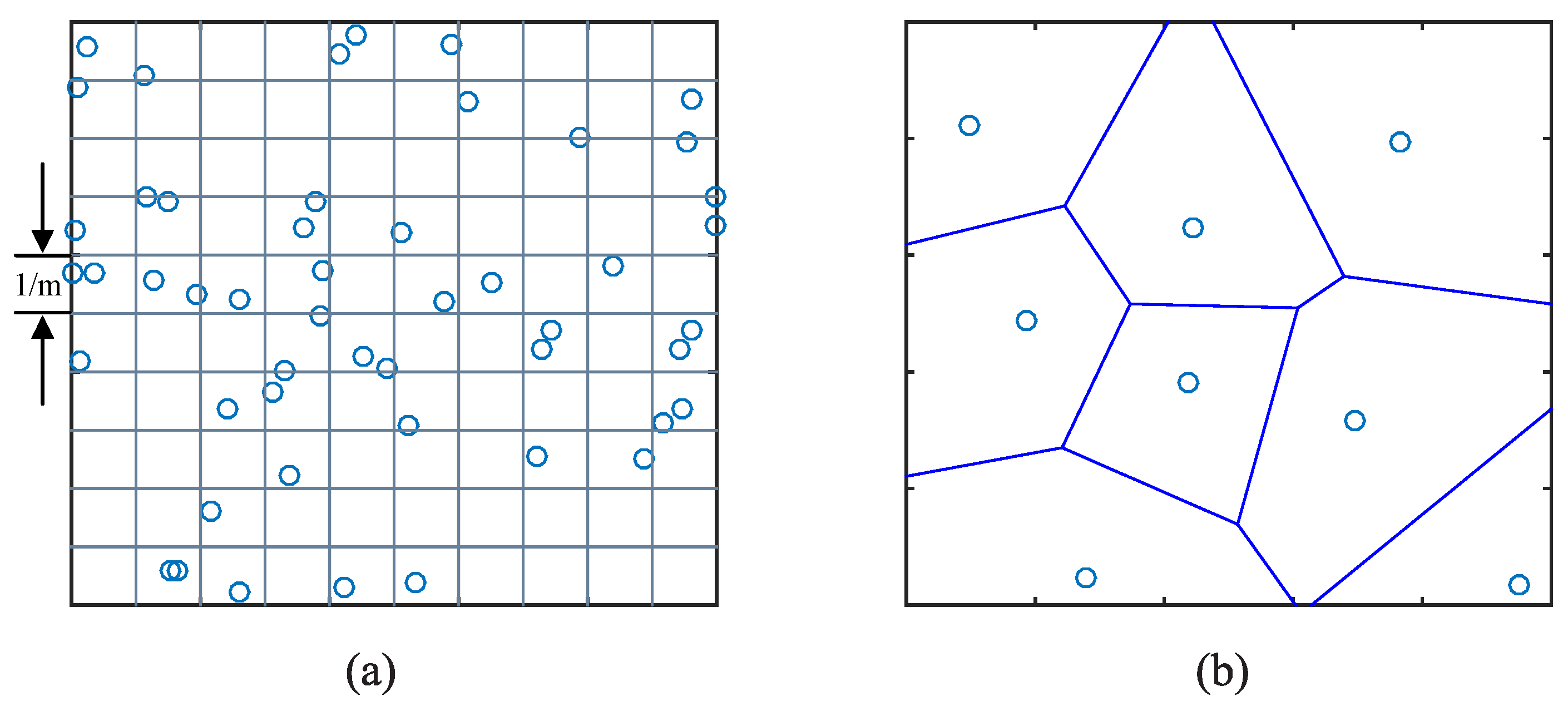
- There are more than one crowdsensing nodes in . The corresponding is calculated by a weight sum of all the sensory data generated in . Considering the distribution of crowdsensing nodes in one grid, we build a voronoi diagram according to the locations of crowdsensing nodes (see Figure 3b), and then calculate the weight sum of sensory data where the area of the divided polygons are weights of sensory data.
- There is no crowdsensing node in . The corresponding is set to null.
2.2. Resolution of Crowdsensing
2.3. Linear Restriction
3. Enhanced Crowdsensing Approach
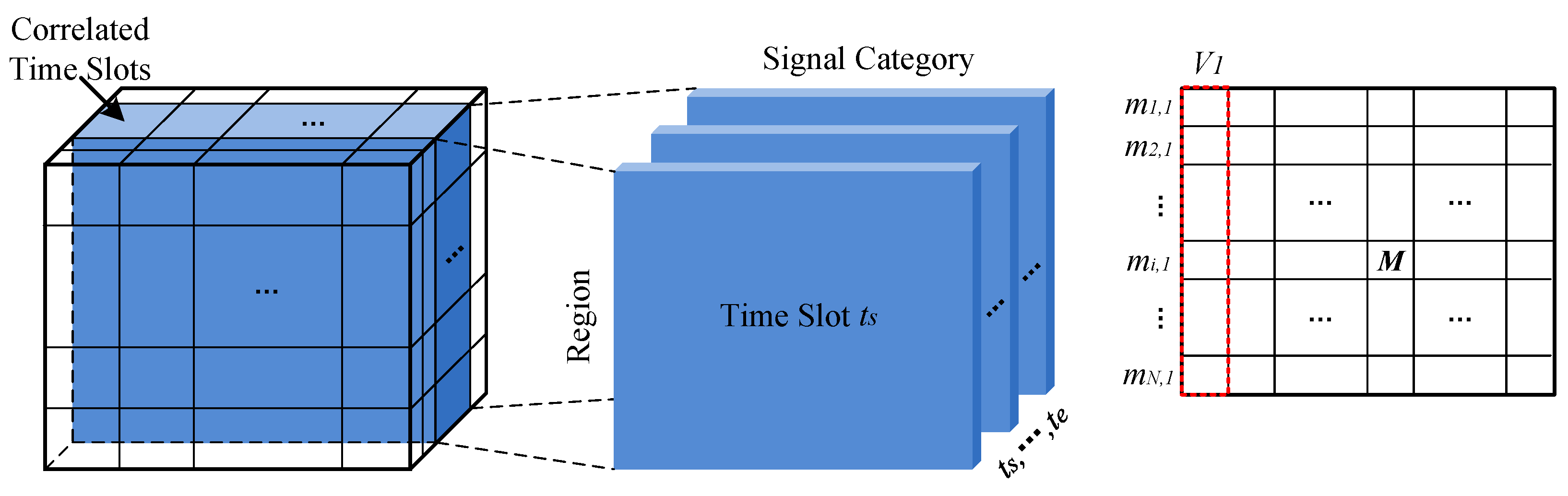
3.1. Data Modeling
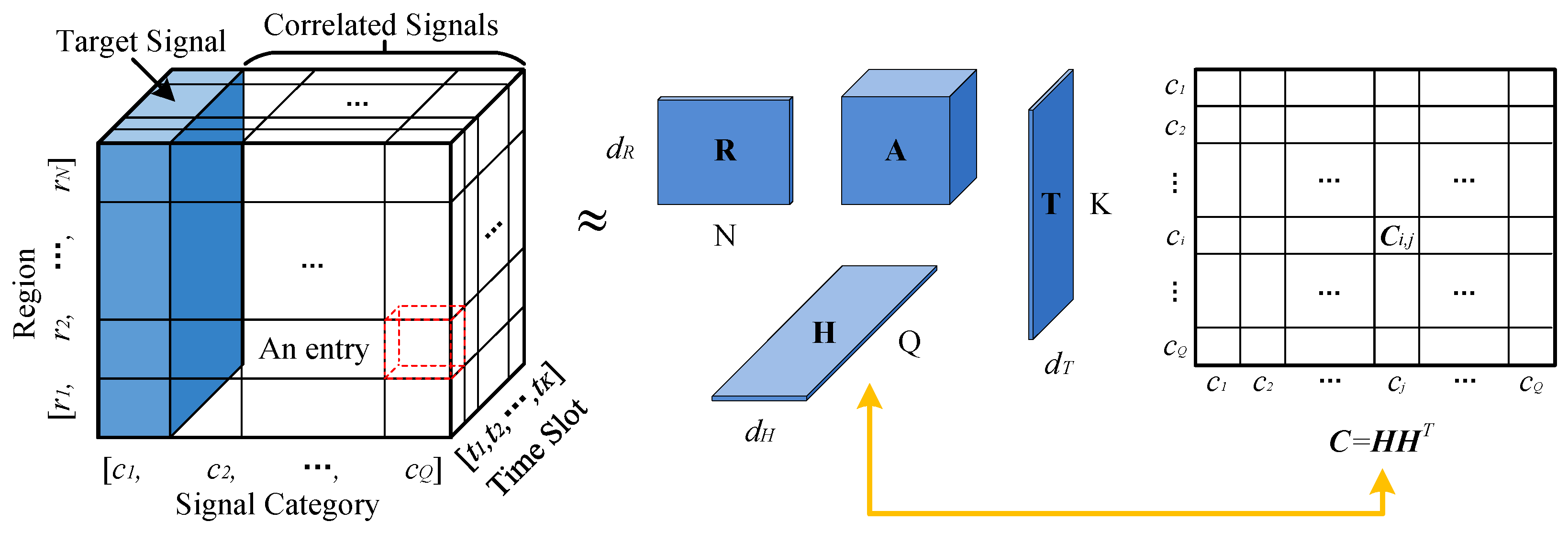
- Region dimension, , denotes N regions which are transferred from grids, one region per grid, .
- Category dimension, , denotes Q signal categorise, where is the target signal and the others are correlated signals.
- Time dimension, , denotes K time slots. Here, we divide the monitoring time period into K time slots and the span of each time slot is decided by the sending intervals of crowdsensing nodes.
3.2. Collaborative Tensor Decomposition
3.3. Correlated Time Slots Combination
4. Numerical Simulation
4.1. Basic Models
4.2. Instance Illustration
4.3. Statistical Results
5. Case Study: Air Quality Monitoring in Beijing
5.1. Data Correlation Analysis
5.2. Data Modelling
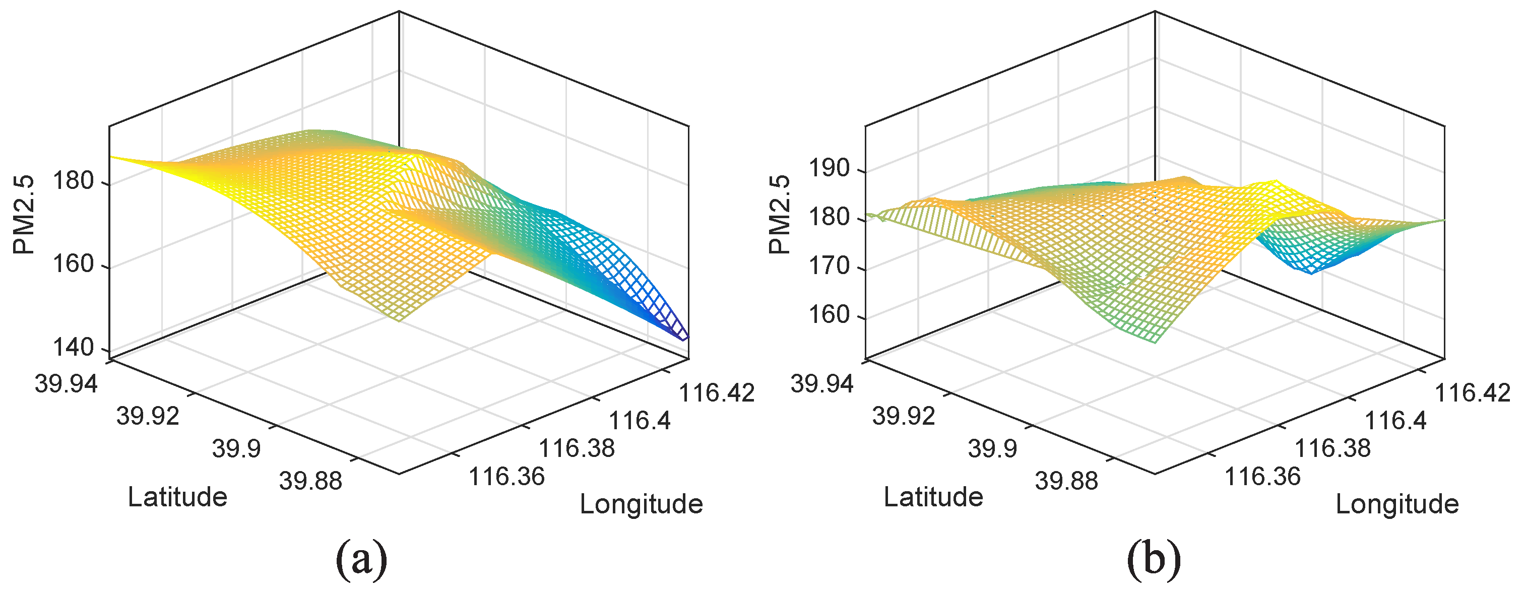
5.3. Comparison of Generated Sensing Images
6. Conclusions
Acknowledgments
Author Contributions
Conflicts of Interest
References
- Yang, X. Urban Remote Sensing: Monitoring, Synthesis and Modeling in the Urban Environment; John Wiley & Sons: Hoboken, NJ, USA, 2011. [Google Scholar]
- Dong, M.; Ota, K.; Liu, A. RMER: Reliable and Energy Efficient Data Collection for Large-scale Wireless Sensor Networks. IEEE Internet Things J. 2016, 3, 511–519. [Google Scholar] [CrossRef]
- Hu, Y.; Dong, M.; Ota, K.; Liu, A. Mobile Target Detection in Wireless Sensor Networks With Adjustable Sensing Frequency. IEEE Syst. J. 2016, 10, 1160–1171. [Google Scholar] [CrossRef]
- Liu, X.; Wei, T.; Liu, A. Fast Program Codes Dissemination for Smart Wireless Software Defined Networks. Sci. Program. 2016, 2016, 1–21. [Google Scholar] [CrossRef]
- Liu, Y.; Dong, M.; Ota, K.; Liu, A. ActiveTrust: Secure and Trustable Routing in Wireless Sensor Networks. IEEE Trans. Inf. Forensics Secur. 2016, 11, 2013–2027. [Google Scholar] [CrossRef]
- Campbell, A.T.; Eisenman, S.B.; Lane, N.D.; Miluzzo, E.; Peterson, R.A.; Lu, H.; Zheng, X.; Musolesi, M.; Fodor, K.; Ahn, G.S. The rise of people-centric sensing. IEEE Internet Comput. 2008, 12, 12–21. [Google Scholar] [CrossRef]
- Tang, Z.; Liu, A.; Li, Z.; Choi, Y.J.; Sekiya, H.; Li, J. A Trust-Based Model for Security Cooperating in Vehicular Cloud Computing. Mobile Inf. Syst. 2016, 2016, 1–22. [Google Scholar] [CrossRef]
- Ganti, R.K.; Ye, F.; Lei, H. Mobile crowdsensing: Current state and future challenges. IEEE Commun. Mag. 2011, 49, 32–39. [Google Scholar] [CrossRef]
- Mitas, L.; Mitasova, H. Spatial interpolation. Geogr. Inf. Syst. Princ. Tech. Manag. Appl. 1999, 1, 481–492. [Google Scholar]
- Liu, L.; Wei, W.; Zhao, D.; Ma, H. Urban resolution: New metric for measuring the quality of urban sensing. IEEE Trans. Mob. Comput. 2015, 14, 2560–2575. [Google Scholar] [CrossRef]
- Lee, K.; Hong, S.; Kim, S.J.; Rhee, I. SLAW: Self-Similar Least-Action Human Walk. IEEE ACM Trans. Netw. 2012, 20, 515–529. [Google Scholar] [CrossRef]
- Wang, L.; Zhang, D.; Wang, Y.; Chen, C. Sparse mobile crowdsensing: Challenges and opportunities. IEEE Commun. Mag. 2016, 54, 161–167. [Google Scholar] [CrossRef]
- Wang, L.; Zhang, D.; Pathak, A.; Chen, C.; Xiong, H.; Yang, D.; Wang, Y. CCS-TA: Quality-guaranteed online task allocation in compressive crowdsensing. In Proceedings of the ACM International Joint Conference on Pervasive and Ubiquitous Computing, Osaka, Japan, 7–11 September 2015; pp. 683–694.
- Zhang, Y.; Roughan, M.; Willinger, W.; Qiu, L. Spatio-temporal compressive sensing and internet traffic matrices. Acm Sigcomm Comput. Commun. Rev. 2009, 39, 267–278. [Google Scholar] [CrossRef]
- Li, Z.; Zhu, Y.; Zhu, H.; Li, M. Compressive Sensing Approach to Urban Traffic Sensing. In Proceedings of the International Conference on Distributed Computing Systems, Minneapolis, MN, USA, 20–24 June 2011; pp. 889–898.
- Rallapalli, S.; Qiu, L.; Zhang, Y.; Chen, Y.C. Exploiting temporal stability and low-rank structure for localization in mobile networks. In Proceedings of the Sixteenth Annual International Conference on Mobile Computing and Networking, Chicago, IL, USA, 20–24 September 2010; pp. 161–172.
- Kong, L.; Xia, M.; Liu, X.Y.; Chen, G.; Gu, Y.; Wu, M.Y.; Liu, X. Data Loss and Reconstruction in Wireless Sensor Networks. IEEE Trans. Parallel Distrib. Syst. 2014, 25, 2818–2828. [Google Scholar] [CrossRef]
- Xu, L.; Hao, X.; Lane, N.D.; Liu, X.; Moscibroda, T. More with less: Lowering user burden in mobile crowdsourcing through compressive sensing. In Proceedings of the ACM International Joint Conference on Pervasive and Ubiquitous Computing, Osaka, Japan, 7–11 September 2015; pp. 659–670.
- Zhang, Y.; Roughan, M.; Willinger, W.; Qiu, L. Spatio-temporal Compressive Sensing and Internet Traffic Matrices. In Proceedings of the ACM SIGCOMM 2009 Conference on Data Communication, Barcelona, Spain, 16–21 August 2009; pp. 267–278.
- Zheng, Y.; Liu, F.; Hsieh, H.P. U-Air: When urban air quality inference meets big data. In Proceedings of the 19th ACM SIGKDD International Conference on Knowledge Discovery and Data Mining, Chicago, IL, USA, 11–14 August 2013; pp. 1436–1444.
- Zheng, Y.; Liu, T.; Wang, Y.; Zhu, Y.; Liu, Y.; Chang, E. Diagnosing New York city’s noises with ubiquitous data. In Proceedings of the 2014 ACM International Joint Conference on Pervasive and Ubiquitous Computing, Seattle, WA, USA, 13–17 September 2014; pp. 715–725.
- Vardoulakis, S.; Fisher, B.E.; Pericleous, K.; Gonzalez-Flesca, N. Modelling air quality in street canyons: A review. Atmos. Environ. 2003, 37, 155–182. [Google Scholar] [CrossRef]
- Kolda, T.G.; Bader, B.W. Tensor decompositions and applications. Soc. Ind. Appl. Math. Rev. 2009, 51, 455–500. [Google Scholar] [CrossRef]
- Mao, X.; Miao, X.; He, Y.; Li, X.Y. Citysee: Urban CO2 monitoring with sensors. In Proceedings of the IEEE INFOCOM International Conference on Computer Communications, Orlando, FL, USA, 25–30 March 2012; pp. 1611–1619.
- Yuan, J.; Zheng, Y.; Xie, X.; Sun, G. Driving with knowledge from the physical world. In Proceedings of the ACM SIGKDD International Conference on Knowledge Discovery and Data Mining, San Diego, CA, USA, 21–24 August 2011; pp. 316–324.


| Parameter | Value |
|---|---|
| Distance alpha | 3 |
| Number of mobile nodes | 6000 |
| Simulation area | |
| Number of waypoints | 6000 |
| Hurst parameter | 0.75 |
| Time duration | 10 h |
| Clustering range | 100 m |
| Levy exponent for pause time | 1 |
| Minimum/maximum pause time | 30 s/1800 s |
| Value Ranges of | Number of Monitoring Stations | |
|---|---|---|
| 13 | 0 | |
| 7 | 1 | |
| 1 | 19 | |
| 1 | 2 | |
© 2017 by the authors; licensee MDPI, Basel, Switzerland. This article is an open access article distributed under the terms and conditions of the Creative Commons Attribution (CC-BY) license (http://creativecommons.org/licenses/by/4.0/).
Share and Cite
Kang, X.; Liu, L.; Ma, H. Enhance the Quality of Crowdsensing for Fine-Grained Urban Environment Monitoring via Data Correlation. Sensors 2017, 17, 88. https://doi.org/10.3390/s17010088
Kang X, Liu L, Ma H. Enhance the Quality of Crowdsensing for Fine-Grained Urban Environment Monitoring via Data Correlation. Sensors. 2017; 17(1):88. https://doi.org/10.3390/s17010088
Chicago/Turabian StyleKang, Xu, Liang Liu, and Huadong Ma. 2017. "Enhance the Quality of Crowdsensing for Fine-Grained Urban Environment Monitoring via Data Correlation" Sensors 17, no. 1: 88. https://doi.org/10.3390/s17010088
APA StyleKang, X., Liu, L., & Ma, H. (2017). Enhance the Quality of Crowdsensing for Fine-Grained Urban Environment Monitoring via Data Correlation. Sensors, 17(1), 88. https://doi.org/10.3390/s17010088