
Epipolar Resampling of Cross-Track Pushbroom Satellite Imagery Using the Rigorous Sensor Model


Abstract
:1. Introduction
2. Theoretical Background
2.1. Linear Pushbroom Imaging
2.2. MPC Model
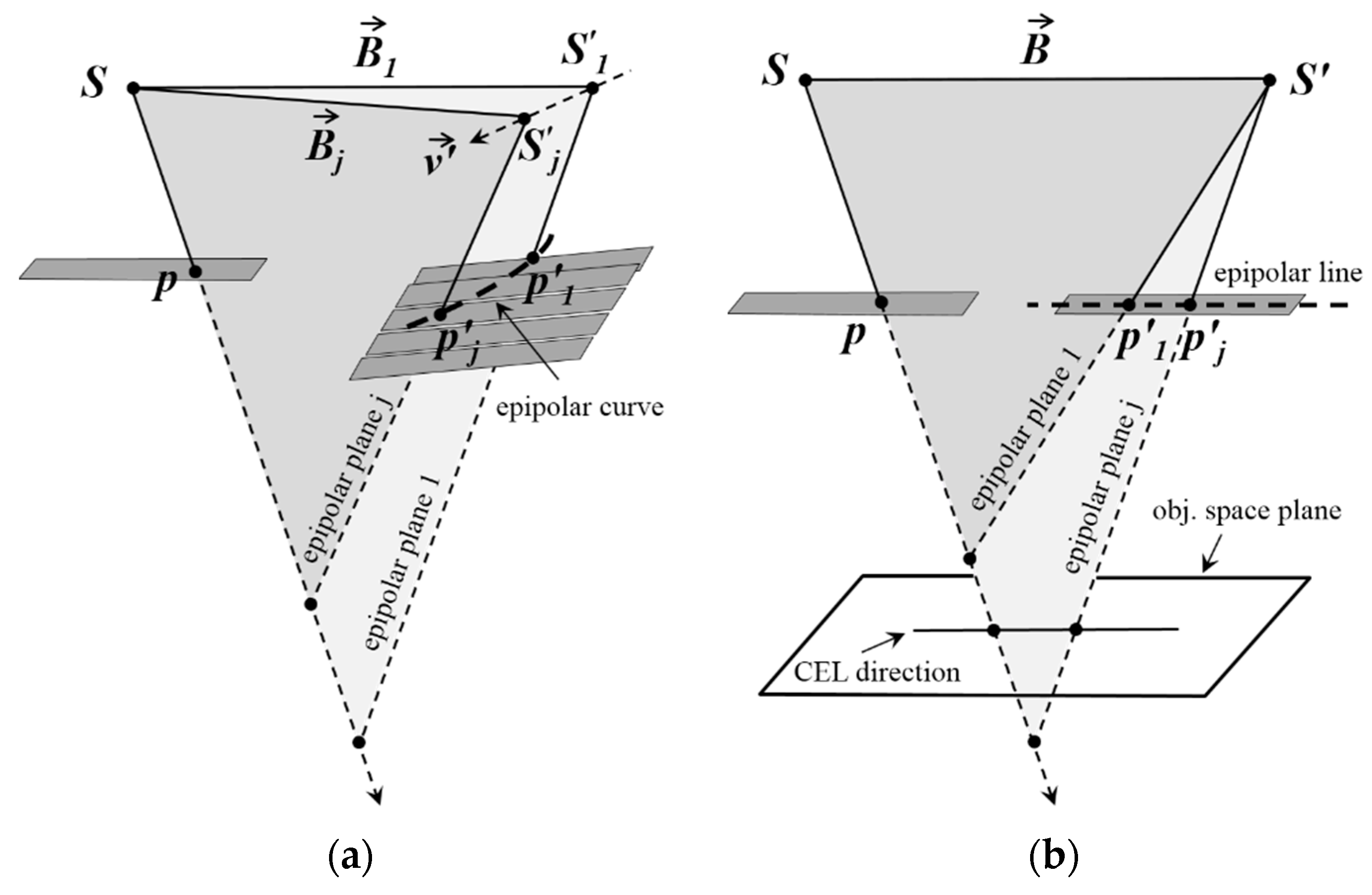
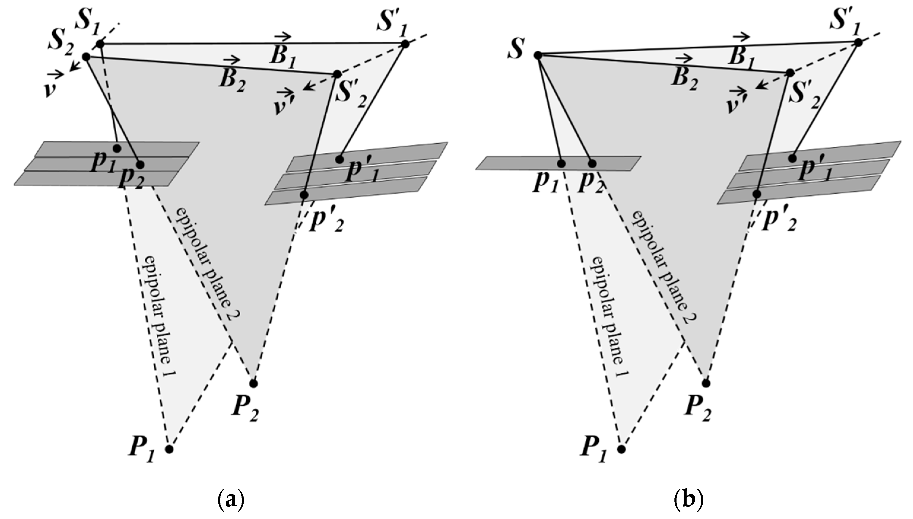
2.3. The EG of Linear Pushbroom Images
3. Proposed Method
- parallelizing scanlines containing the CIPs with their IBs to produce straight epipolar lines,
- parallelizing the epipolar lines of all CIPs with each other to eliminate the vertical parallax of CIPs, and,
- correcting the scale of the normalized scenes.
3.1. Producing Straight Epipolar Lines
3.2. Eliminating the Vertical Parallax of CIPs
3.3. Correcting the Scale of the Normalized Scenes
4. Study Area and Data Used
5. Results
6. Discussion
7. Conclusions
Author Contributions
Conflicts of Interest
Abbreviations
| IB | Instantaneous Baseline |
| CIPs | Conjugate Image Points |
| EG | Epipolar Geometry |
| DEM | Digital Elevation Model |
| ROP | Relative Orientation Parameters |
| EOP | Exterior Orientation Parameters |
| IOP | Interior Orientation Parameters |
| RFM | Rational Function Model |
| ACEL | Approximate Conjugate Epipolar Lines |
| RPCs | Rational Function Coefficients |
| MPC | Multiple projection Centers |
| PP | Parallel Projection |
| CCDs | Charged Coupled Devices |
| CMOS | Complementary Metal-Oxide Semiconductor |
| GCPs | Ground Control Points |
| IRF | Image Reference Frame |
| GRF | Ground Reference Frame |
| SRF | Sensor Reference Frame |
| PRF | Platform Reference Frame |
| CEL | Conjugate Epipolar Lines |
| CoCP | Control Conjugate Points |
| ChCP | Check Conjugate Points |
References
- Morgan, M. Epipolar Resampling of Linear Array Scanner Scenes. Ph.D. Thesis, University of Calgary, Calgary, AB, Canada, 2004. [Google Scholar]
- Kornus, W.; Alamús, R.; Ruiz, A.; Talaya, J. DEM generation from SPOT-5 3-fold along track stereoscopic imagery using autocalibration. ISPRS J. Photogramm. Remote Sens. 2006, 60, 147–159. [Google Scholar] [CrossRef]
- Cho, W.; Schenk, T.; Madani, M. Resampling Digital Imagery to Epipolar Geometry. Int. Arch. Photogramm. Remote Sens. 1992, 29, 404–408. [Google Scholar]
- Torr, P.H.S. Bayesian model estimation and selection for epipolar geometry and generic manifold fitting. Int. J. Comput. Vis. 2002, 50, 35–61. [Google Scholar] [CrossRef]
- Kim, T. A Study on the Epipolarity of Linear Pushbroom Images. Photogramm. Eng. Remote Sens. 2000, 66, 961–966. [Google Scholar]
- Heipke, C.; Kornus, W.; Pfannenstein, A. The Evaluation of MEOSS Airborne Three-line Scanner Imagery: Processing chain and results. Photogramm. Eng. Remote Sens. 1996, 62, 293–299. [Google Scholar]
- Gupta, R.; Hartley, R.I. Linear Pushbroom Cameras. IEEE Trans. Pattern Anal. Mach. Intell. 1997, 19, 963–975. [Google Scholar] [CrossRef]
- Habib, A.F.; Morgan, M.; Jeong, S.; Kim, K.O. Analysis of Epipolar Geometry in Linear Array Scanner Scenes. Photogramm. Record. 2005, 20, 27–47. [Google Scholar] [CrossRef]
- Kratky, V. Rigorous Stereo Photogrammetric Treatment of SPOT Images, SPOT 1-Utilisation des Images, Bilan, Resultats; CNES: Paris, France, 1987; pp. 1195–1204. [Google Scholar]
- Lee, H.Y.; Park, W. A new epipolarity model based on the simplified pushbroom sensor model. Int. Achieves Photogramm. Remote Sens. Spat. Inf. Sci. 2002, 34, 631–636. [Google Scholar]
- Morgan, M.; Kim, K.; Jeong, S.; Habib, A. Indirect epipolar resampling of scenes using parallel projection modeling of linear array scanners. Int. Achieves Photogramm. Remote Sens. Spat. Inf. Sci. 2004, 35, 508–513. [Google Scholar]
- Oh, J.; Lee, W.H.; Toth, C.K.; Grejner-Brzezinska, D.A.; Lee, C. A Piecewise Approach to Epipolar Resampling of Pushbroom Satellite Images Based on RPC. Photogramm. Eng. Remote Sens. 2010, 76, 1353–1363. [Google Scholar] [CrossRef]
- Wang, M.; Hub, F.; Li, J. Epipolar Resampling of Linear Pushbroom Satellite Imagery by a New Epipolarity Model. ISPRS J. Photogramm. Remote Sens. 2011, 66, 347–355. [Google Scholar] [CrossRef]
- Koh, J.W.; Yang, H.S. Unified piecewise epipolar resampling method for pushbroom satellite images. EURASIP J. Image Video Process. 2016, 1. [Google Scholar] [CrossRef]
- Fraser, C.S.; Yamakawa, T. Insights into the affine model for high-resolution satellite sensor orientation. ISPRS J. Photogramm. Remote Sens. 2004, 58, 275–288. [Google Scholar] [CrossRef]
- Morgan, M.; Kim, K.; Jeong, S.; Habib, A. Epipolar geometry of linear array scanners moving with constant velocity and constant attitude. Int. Achieves Photogramm. Remote Sens. Spat. Inf. Sci. 2004, 35, 52–57. [Google Scholar]
- Morgan, M.; Kim, K.; Jeong, S.; Habib, A. Epipolar resampling of spaceborne linear array scanner scenes using parallel projection. Photogramm. Eng. Remote Sens. 2006, 72, 1255–1263. [Google Scholar] [CrossRef]
- Jaehong, O.H.; Shin, S.W.; Kim, K. Direct epipolar image generation from IKONOS stereo imagery based on RPC and parallel projection model. Korean J. Remote Sens. 2006, 22, 451–456. [Google Scholar]
- Habib, A.F.; Kim, E.M.; Morgan, M.; Couloigner, I. DEM generation from high resolution satellite imagery using parallel projection model. Int. Achieves Photogramm. Remote Sens. Spat. Inf. Sci. 2004, 35, 393–398. [Google Scholar]
- Baltsavias, E.; Pateraki, M.; Zhang, L. Radiometric and geometric evaluation of Ikonos Geo images and their use for 3D building modeling. In Proceedings of the Joint ISPRS Workshop High Resolution Mapping from Space 2001, Hanover, Germany, 19–21 September 2001.
- Fraser, C.; Hanley, H.; Yamakawa, T. Sub-Metre Geopositioning with IKONOS GEO Imagery. In Proceedings of the Joint ISPRS Workshop High Resolution Mapping from Space 2001, Hanover, Germany, 19–21 September 2001.
- Fraser, C.; Hanley, H. Bias Compensation in Rational Functions for IKONOS Satellite Imagery. J. Photogramm. Eng. Remote Sens. 2003, 69, 53–57. [Google Scholar] [CrossRef]
- Tao, V.; Hu, Y. A Comprehensive Study for Rational Function Model for Photogrammetric Processing. J. Photogramm. Eng. Remote Sens. 2001, 67, 1347–1357. [Google Scholar]
- Habib, A.F.; Morgan, M.; Jeong, S.; Kim, K.O. Epipolar Geometry of Line Cameras Moving with Constant Velocity and Attitude. ETRI J. 2005, 27, 172–180. [Google Scholar] [CrossRef]
- Lee, Y.; Habib, A. Pose Estimation of Line Cameras Using Linear Features. In Proceedings of the ISPRS Symposium of PCV’02 Photogrammetric Computer Vision, Graz, Austria, 9–13 September 2002.
- Lee, C.; Theiss, H.; Bethel, J.; Mikhail, E. Rigorous Mathematical Modeling of Airborne Pushbroom Imaging Systems. J. Photogramm. Eng. Remote Sens. 2000, 66, 385–392. [Google Scholar]
- Valadan Zoej, M.J.; Petrie, G. Mathematical Modeling and Accuracy Testing of SPOT Level 1B Stereo Pairs. Photogramm. Record. 1998, 16, 67–82. [Google Scholar] [CrossRef]
- Valadan Zoej, M.J.; Sadeghian, S. Orbital Parameter Modeling Accuracy Testing of Ikonos Geo Image. Photogramm. J. Finl. 2003, 18, 70–80. [Google Scholar]
- Valadan Zoej, M.J. Photogrammetric Evaluation of Space Linear Array Imagery for Medium Scale Topographic Mapping. Ph.D. Thesis, University of Glasgow, Glasgow, UK, 1997. [Google Scholar]
- Wolf, P.R.; Dewitt, B.A. Elements of Photogrammetry with Applications in GIS, 3/e; McGraw-Hill: Toronto, ON, Canada, 2000; p. 608. [Google Scholar]
- Aguilar, M.A.; Saldaña, M.; Aguilar, F.J. Generation and quality assessment of stereo-extracted DSM from GeoEye-1 and WorldView-2 imagery. IEEE Trans. Geosci. Remote Sens. 2013, 52, 1259–1271. [Google Scholar] [CrossRef]
- Toutin, T. Comparison of 3D Physical and Empirical Models for Generating DSMs from Stereo HR Images. Photogramm. Eng. Remote Sens. 2006, 72, 597–604. [Google Scholar] [CrossRef]
- Deltsidis, P.; Ioannidis, C. Orthorectification of World View 2 Stereo Pair Using A New Rigorous Orientation Model. In Proceedings of the ISPRS Hanover 2011 Workshop, Hanover, Germany, 14–17 June 2011.
- Crespi, M.; Fratarcangeli, F.; Giannone, F.; Pieralice, F. A new rigorous model for high-resolution satellite imagery orientation: Application to EROS A and QuickBird. Int. J. Remote Sens. 2012, 33, 2321–2354. [Google Scholar] [CrossRef]
- Orun, A.B.; Natarajan, K. A Modified Bundle Adjustment Software for SPOT Imagery and Photography: Tradeoff. Photogramm. Eng. Remote Sens. 1994, 60, 1431–1437. [Google Scholar]
- Jannati, M.; Valadan Zoej, M.J. Introducing genetic modification concept to optimize rational function models (RFMs) for georeferencing of satellite imagery. GISci. Remote Sens. 2015, 52, 510–525. [Google Scholar] [CrossRef]
- Long, T.; Jiao, W.; He, G. RPC Estimation via L1-Norm-Regularized Least Squares (L1LS). IEEE Trans. Geosci. Remote Sens. 2015, 53, 4554–4567. [Google Scholar] [CrossRef]
- Yavari, S.; Valadan Zoej, M.J.; Mohammadzadeh, A.; Mokhtarzade, M. Particle Swarm Optimization of RFM for Georeferencing of Satellite Images. IEEE Geosci. Remote Sens. Lett. 2012, 10, 135–139. [Google Scholar] [CrossRef]
- Valadan Zoej, M.J.; Mokhtarzade, M.; Mansourian, A.; Ebadi, H.; Sadeghian, S. Rational Function Optimization Using Genetic Algorithms. Int. J. Appl. Earth Observ. Geoinf. 2007, 9, 403–413. [Google Scholar] [CrossRef]


| Attitude Parameters | ω | ϕ | K | ||||||
|---|---|---|---|---|---|---|---|---|---|
| Statistics | Value | p-Value | Std-Err | Value | p-Value | Std-Err | Value | p-Value | Std-Err |
| β0 | 0.449 | 4.4 × 10−201 | 1.0 × 10⁻⁷ | 0.140 | 1.5 × 10−105 | 2.1 × 10⁻⁵ | 0.061 | 2.4 × 10−105 | 9.3 × 10⁻⁶ |
| β1 | −1.6 × 10⁻⁷ | 9.3 × 10−99 | 3.9 × 10⁻¹¹ | −4.8 × 10⁻¹⁰ | 9.5 × 10⁻⁴ | 7.9 × 10⁻⁹ | −2.1 × 10⁻⁸ | 7.7 × 10⁻⁷ | 3.5 × 10⁻⁹ |
| β2 | 1.2 × 10⁻⁸ | 1.6 × 10−55 | 5.5 × 10⁻¹¹ | 2.6 × 10⁻⁶ | 2.6 × 10−56 | 1.1 × 10⁻⁸ | 1.1 × 10⁻⁶ | 2.7 × 10−56 | 4.9 × 10⁻⁹ |
| β3 | 3.6 × 10⁻¹⁴ | 1.6 × 10⁻⁷ | 5.6 × 10⁻¹⁵ | −1.0 × 10⁻¹¹ | 3.8 × 10⁻¹¹ | 1.1 × 10⁻¹² | −5.1 × 10⁻¹² | 5.0 × 10⁻¹² | 5.0 × 10⁻¹³ |
| β4 | 6.0 × 10⁻¹³ | 1.3 × 10−44 | 5.6 × 10⁻¹⁵ | 4.4 × 10⁻¹² | 4.6 × 10⁻⁵ | 1.1 × 10⁻¹² | 2.0 × 10⁻¹² | 2.9 × 10⁻⁵ | 5.0 × 10⁻¹³ |
| β5 | 1.0 × 10⁻¹³ | 3.4 × 10⁻¹⁵ | 7.5 × 10⁻¹⁵ | 1.8 × 10⁻¹¹ | 5.3 × 10⁻¹⁴ | 1.5 × 10⁻¹² | 8.6 × 10⁻¹² | 1.2 × 10⁻¹⁴ | 6.7 × 10⁻¹³ |
| R2 | 1.00 | 1.00 | 1.00 | ||||||
| (s) | 9.0 × 10⁻⁸ | 1.8 × 10⁻⁶ | 8.1 × 10⁻⁷ | ||||||
| Functional form: Y = β0 + β1 × i + β2 × l + β3 × i × l + β4 × i2 + β5 × l2 | |||||||||
| Dataset | Isfahan | Zanjan | Fars | |||
|---|---|---|---|---|---|---|
| Platform | SPOT-1 | SPOT-3 | Rapid Eye-2 | |||
| Sensor | HRV | HRV | Green Band † | |||
| Acquisition date | August 1987 | January 1987 | July 1993 | July 1993 | March 2010 | March 2010 |
| Pointing angle | 24.7° W | 20.84° E | 19.01° W | 16.66° E | 19.64° W | 7.09° E |
| Ground resolution | 10 m | 10 m | 6.5 m | |||
| Base to height ratio | 0.974 | 0.737 | 0.534 | |||
| Elevation relief | 687.2 m | 654.2 m | 842.6 m | |||
| Cloud percentage | 0% | >5% | >1% | |||
| Dataset | # Ctrls | # Chks | Space Resection (pix) | Space Intersection (m) | ||||||
|---|---|---|---|---|---|---|---|---|---|---|
| δr | δc | δrc | δX | δY | δXY | δZ | ||||
| Isfahan | Scene 1 | 15 | 20 | 0.65 | 0.49 | 0.81 | 6.11 | 6.58 | 8.97 | 6.73 |
| Scene 2 | 15 | 20 | 0.76 | 0.54 | 0.93 | |||||
| Zanjan | Scene 1 | 15 | 16 | 0.73 | 0.62 | 0.95 | 5.66 | 6.12 | 8.33 | 5.57 |
| Scene 2 | 15 | 16 | 0.56 | 0.7 | 0.89 | |||||
| Fars | Scene 1 | 15 | 19 | 0.52 | 0.4 | 0.65 | 3.31 | 4.37 | 5.48 | 4.21 |
| Scene 2 | 15 | 19 | 0.55 | 0.38 | 0.67 | |||||
| Dataset | Isfahan | Zanjan | Fars | |||||||||
|---|---|---|---|---|---|---|---|---|---|---|---|---|
| Experiment Number | 1 | 2 | 3 | 4 | 5 | 6 | 7 | 8 | 9 | 10 | 11 | 12 |
| Number of CoCP | 8 | 10 | 12 | 16 | 8 | 10 | 12 | 16 | 8 | 10 | 12 | 16 |
| Number of ChCP | 32 | 30 | 28 | 24 | 32 | 30 | 28 | 24 | 32 | 30 | 28 | 24 |
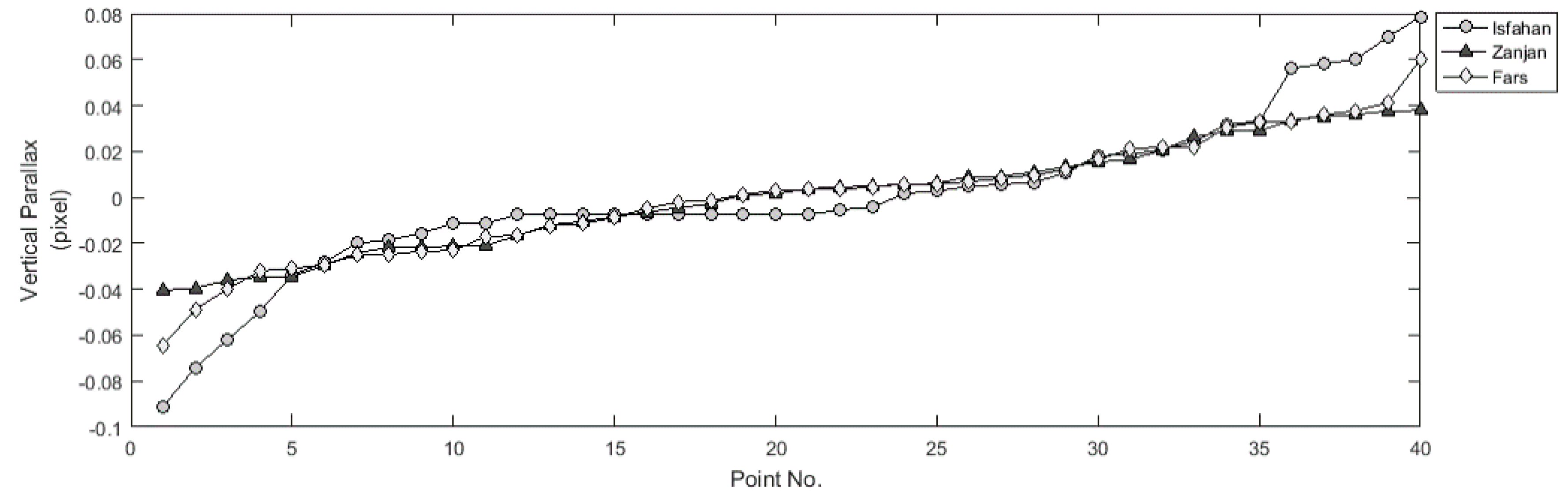
| Mean |PV|, pixels | 0.03 | 0.02 | 0.00 | 0.00 | 0.02 | 0.01 | 0.01 | 0.00 | 0.03 | 0.02 | 0.02 | 0.01 |
| Max |PV|, pixels | 0.17 | 0.09 | 0.00 | 0.00 | 0.06 | 0.04 | 0.03 | 0.02 | 0.08 | 0.06 | 0.07 | 0.05 |
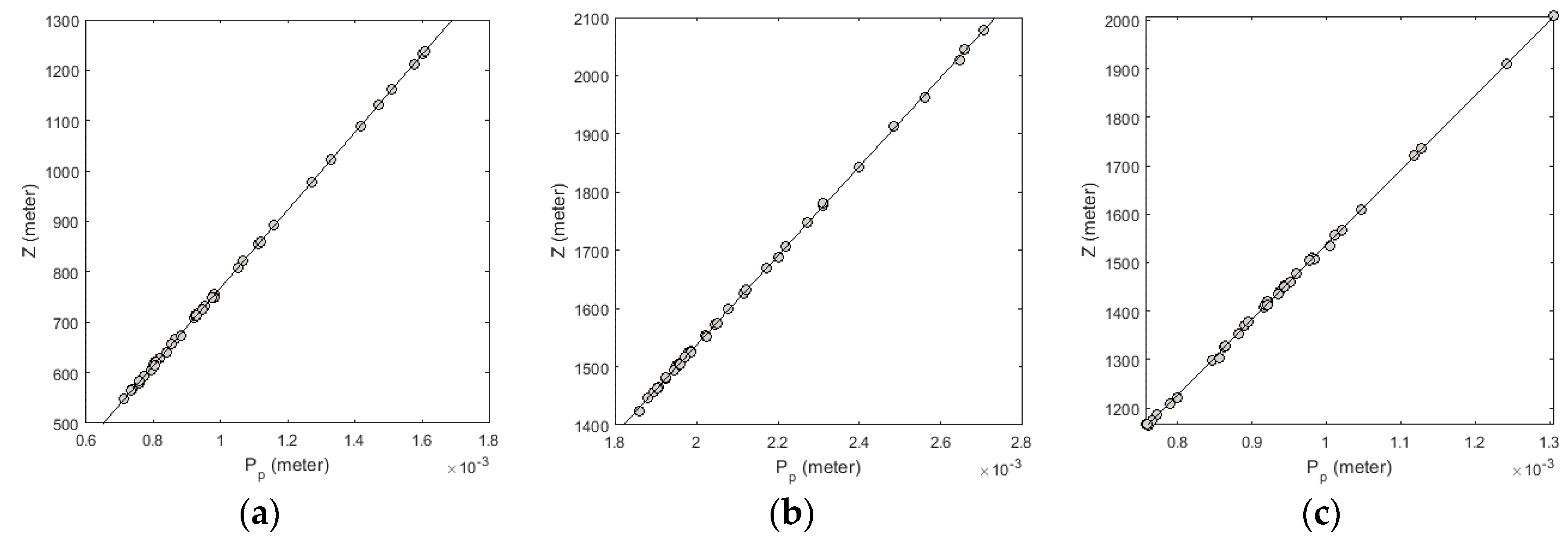
| (line fitting of PH and Z), m | 5.72 | 1.93 | 1.47 | 0.76 | 3.55 | 2.15 | 1.46 | 1.31 | 6.31 | 5.44 | 4.97 | 3.83 |
© 2017 by the authors; licensee MDPI, Basel, Switzerland. This article is an open access article distributed under the terms and conditions of the Creative Commons Attribution (CC-BY) license (http://creativecommons.org/licenses/by/4.0/).
Share and Cite
Jannati, M.; Valadan Zoej, M.J.; Mokhtarzade, M. Epipolar Resampling of Cross-Track Pushbroom Satellite Imagery Using the Rigorous Sensor Model. Sensors 2017, 17, 129. https://doi.org/10.3390/s17010129
Jannati M, Valadan Zoej MJ, Mokhtarzade M. Epipolar Resampling of Cross-Track Pushbroom Satellite Imagery Using the Rigorous Sensor Model. Sensors. 2017; 17(1):129. https://doi.org/10.3390/s17010129
Chicago/Turabian StyleJannati, Mojtaba, Mohammad Javad Valadan Zoej, and Mehdi Mokhtarzade. 2017. "Epipolar Resampling of Cross-Track Pushbroom Satellite Imagery Using the Rigorous Sensor Model" Sensors 17, no. 1: 129. https://doi.org/10.3390/s17010129
APA StyleJannati, M., Valadan Zoej, M. J., & Mokhtarzade, M. (2017). Epipolar Resampling of Cross-Track Pushbroom Satellite Imagery Using the Rigorous Sensor Model. Sensors, 17(1), 129. https://doi.org/10.3390/s17010129