
Fast Object Motion Estimation Based on Dynamic Stixels


Abstract
:
1. Introduction
- Compact: significant reduction in data volume.
- Complete: information of interest is preserved.
- Stable: small changes in underlying data do not cause rapid changes in the representation.
- Robust: outliers have little or no impact on the resulting representation.
- Good reconstruction quality in terms of computed depth. Free space computation without disparity maps has some drawbacks involving low depth accuracy. Object reconstruction and the detection scheme improve the correction of stixel depths and remove false obstacles.
- Better detection results and faster tracking than other methods, as in [7].
- Better robustness after changes between images (for example, when faced with a low frame rate).
- Stixel obstacle detection in crowded pedestrian areas provides reliability and speed at the same time.
2. Previous Work
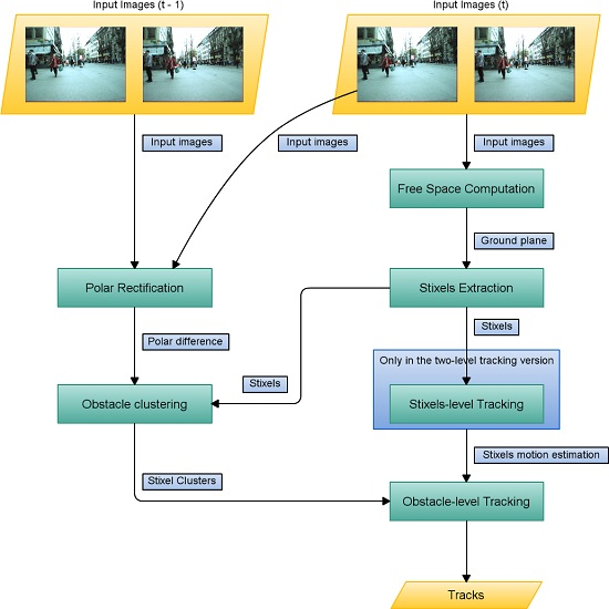
3. Method
- Free space is computed from a stereo pair in order to estimate the ground plane.
- Stixels are obtained and placed on the ground based on their depth and position.
- At the first level, the stixels are tracked as per [7]. The set of stixels in the current frame is compared and matched to the previous one.
- Stixels are clustered based on their projected position in 3D.
- Using these clusters and the tracked stixels, tracking is performed at the stixel level. Obstacles in the scene and their velocities are calculated, and their positions in previous frames are recorded to estimate their future motion.
- In the second level, tracking is performed only at the object level. Each obstacle is compared to obstacles detected in previous frames, meaning that stixel-level tracking is no longer needed.
3.1. Computing Stixels
- The algorithm’s input is a calibrated stereo image pair.
- A Lambertian surface is assumed.
- The ground is planar, at least locally.
- Objects are mainly vertical with a limited height.
- The stereo rig has negligible roll with respect to the ground plane.
3.1.1. Computing the Free Space
3.1.2. Stixel Extraction
3.2. Tracking
- All stixels are assumed to be properly estimated.
- The maximum object speed is limited, so the search range between stixels is constrained. As there is just one stixel per column, matching is limited to a search in the u direction.
- Since two consecutive frames are relatively close, the same stixel at time t and should look similar, including its height. Section 4.3.2 shows that this restriction can be reduced depending on the tracking approach.
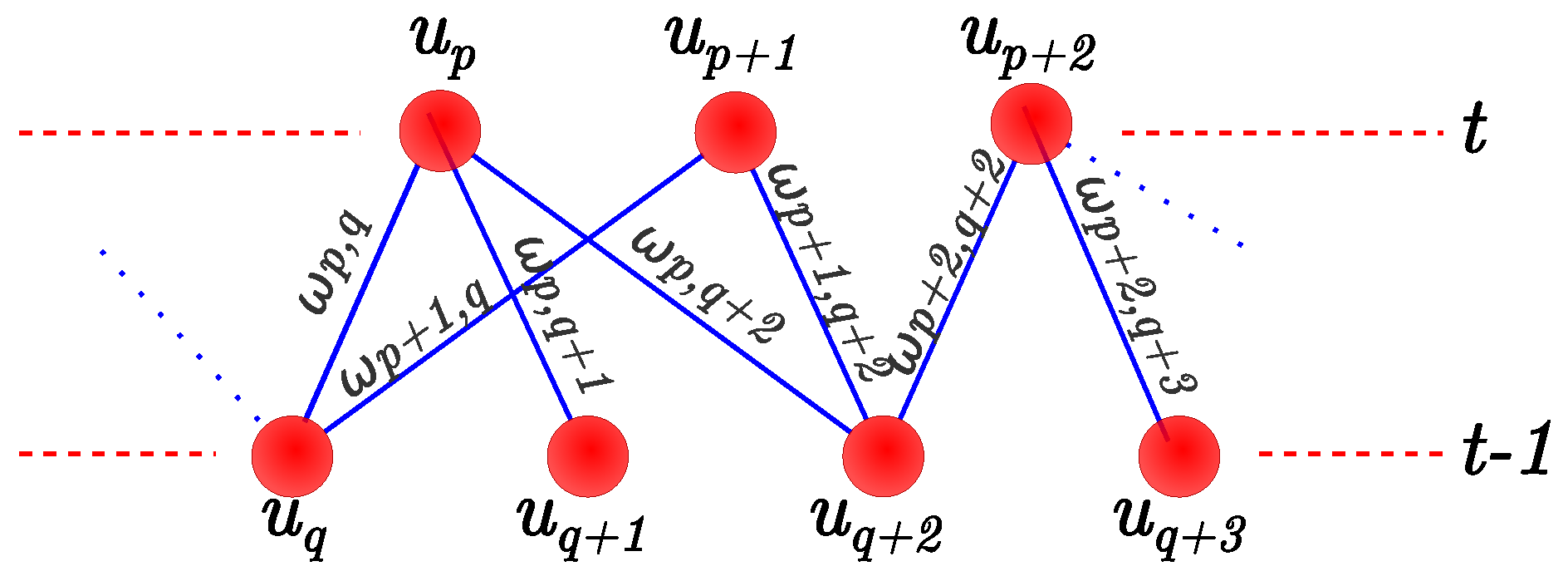
3.2.1. Stixel-Level Tracking
- , where parameter indicates the maximum stixel displacement between frames; and is the position in 3D coordinates in the longitudinal axis X, which grows from left to right in 3D Cartesian coordinates. Axis Y is the vertical axis, which grows downwards, and the Z axis starts from the local coordinate system of the robot towards its front.
- is not the first frame in which stixel appears.
- Stixels and are not occluded.
- .
3.2.2. Sum of Absolute Differences
3.2.3. Histogram Matching
3.2.4. Height Difference
3.3. Obstacle-Level Tracking
3.3.1. Clustering
| Algorithm 1 Clustering algorithm. |
|
Obstacle Aggregation
| Algorithm 2 Aggregation algorithm. |
|
Obstacle Filtering
- The points obtained should be the same for the entire cycle.
- Features in must be in the same row as . The same applies to and .
- The distances between features in frames t and should be similar.
3.3.2. Tracking
Two-Level Tracking Approach
| Algorithm 3 Two-level tracking algorithm. |
|
Object Tracking Approach
3.3.3. Integration with the Navigation Subsystem
4. Results
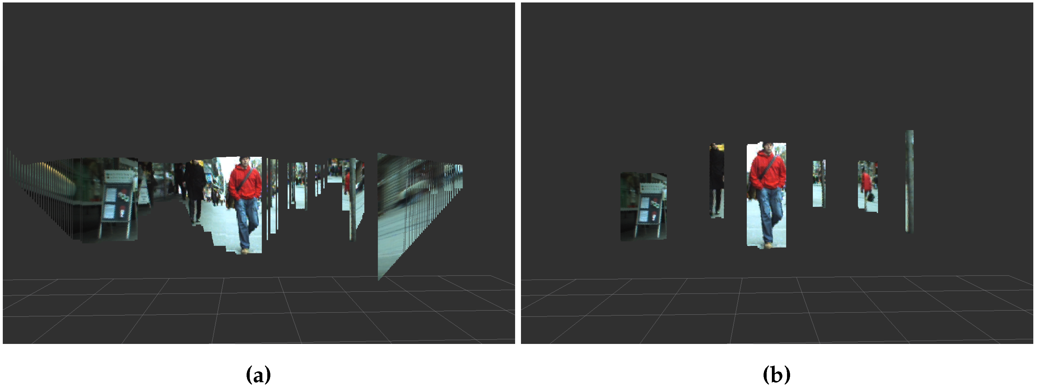
- The quality of the clustering process.
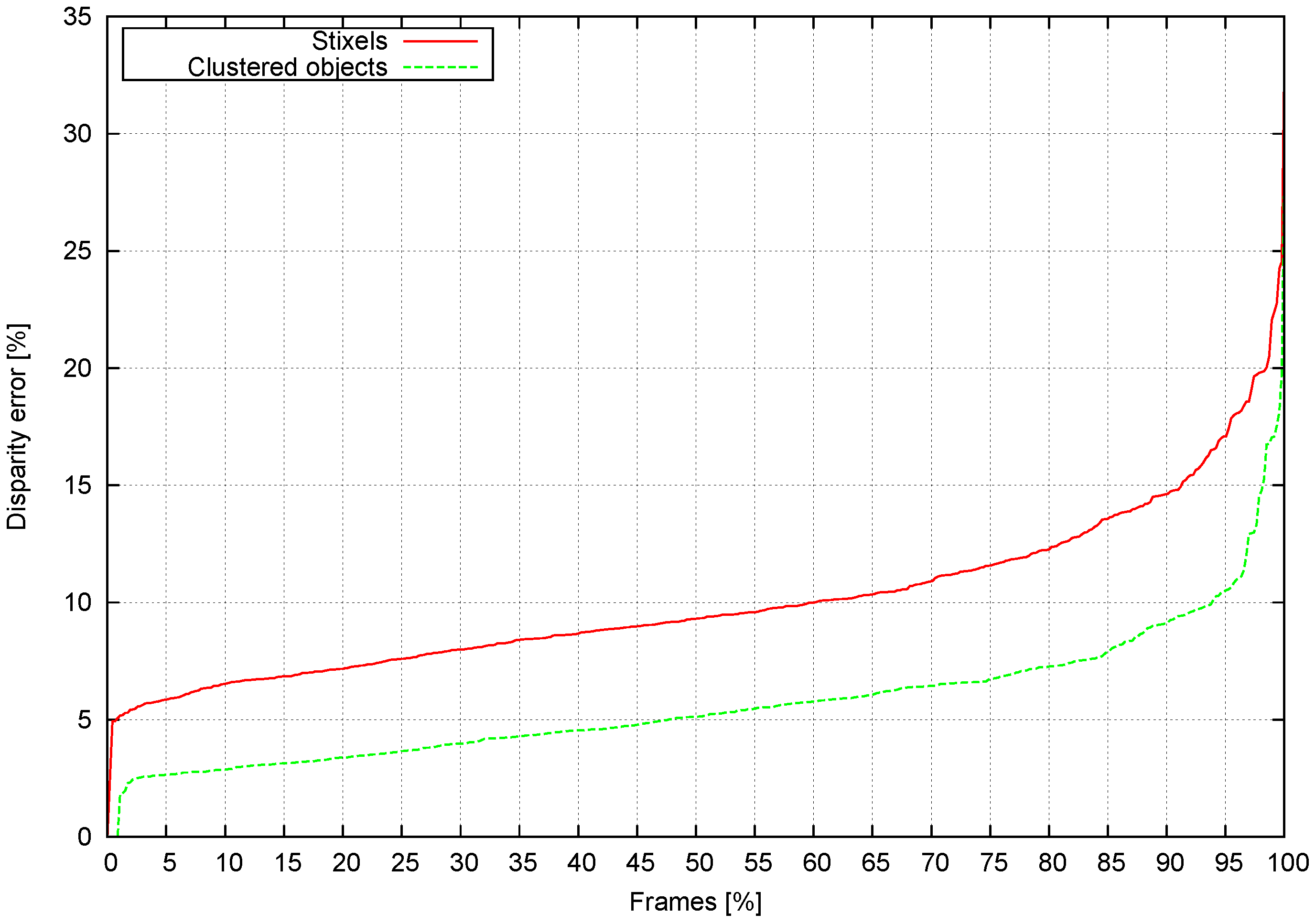
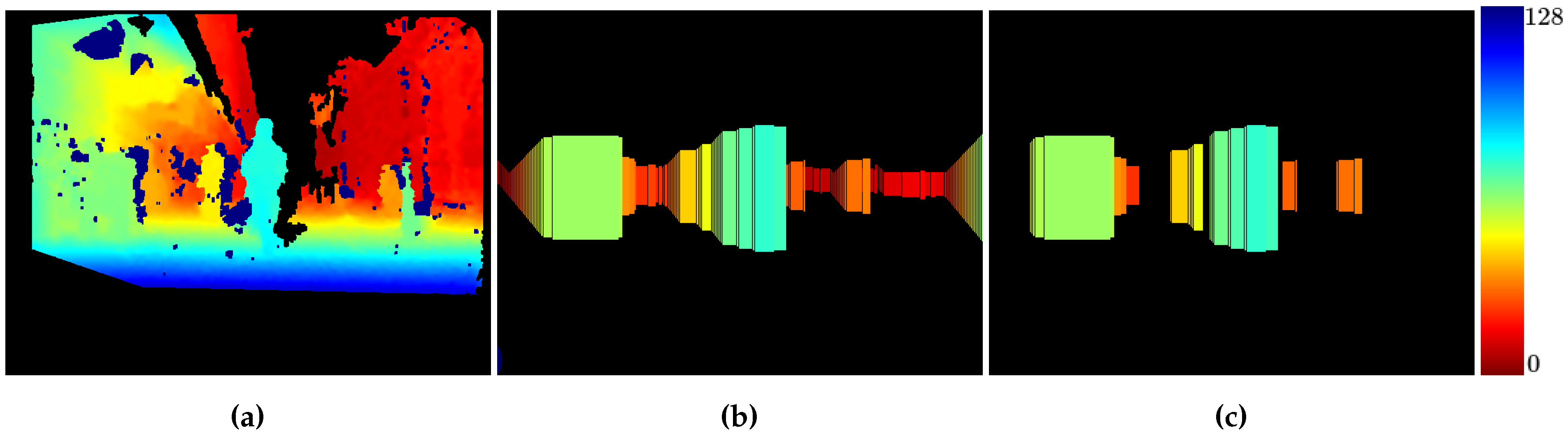
- Stixel depth accuracy compared to object-level tracking.
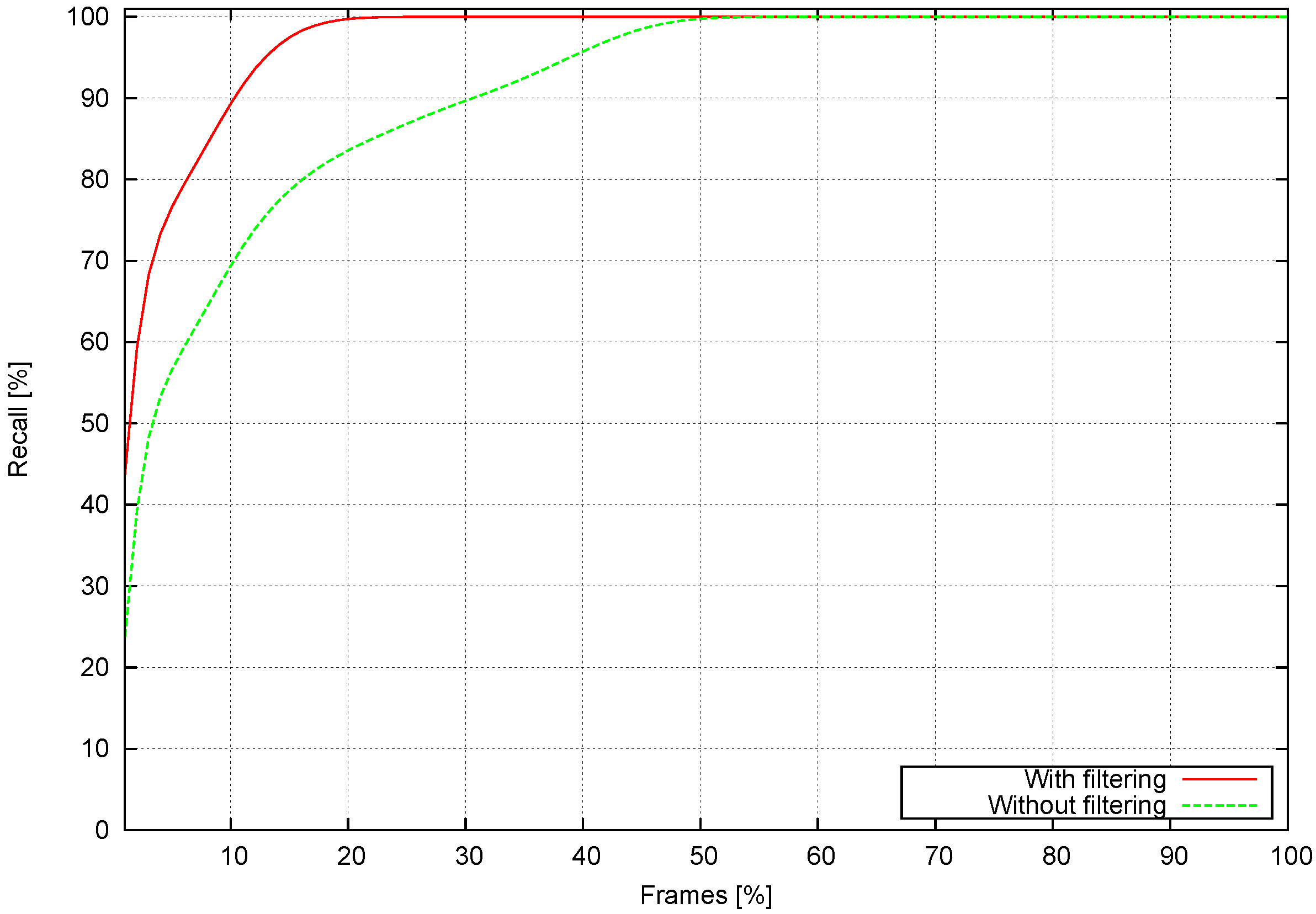
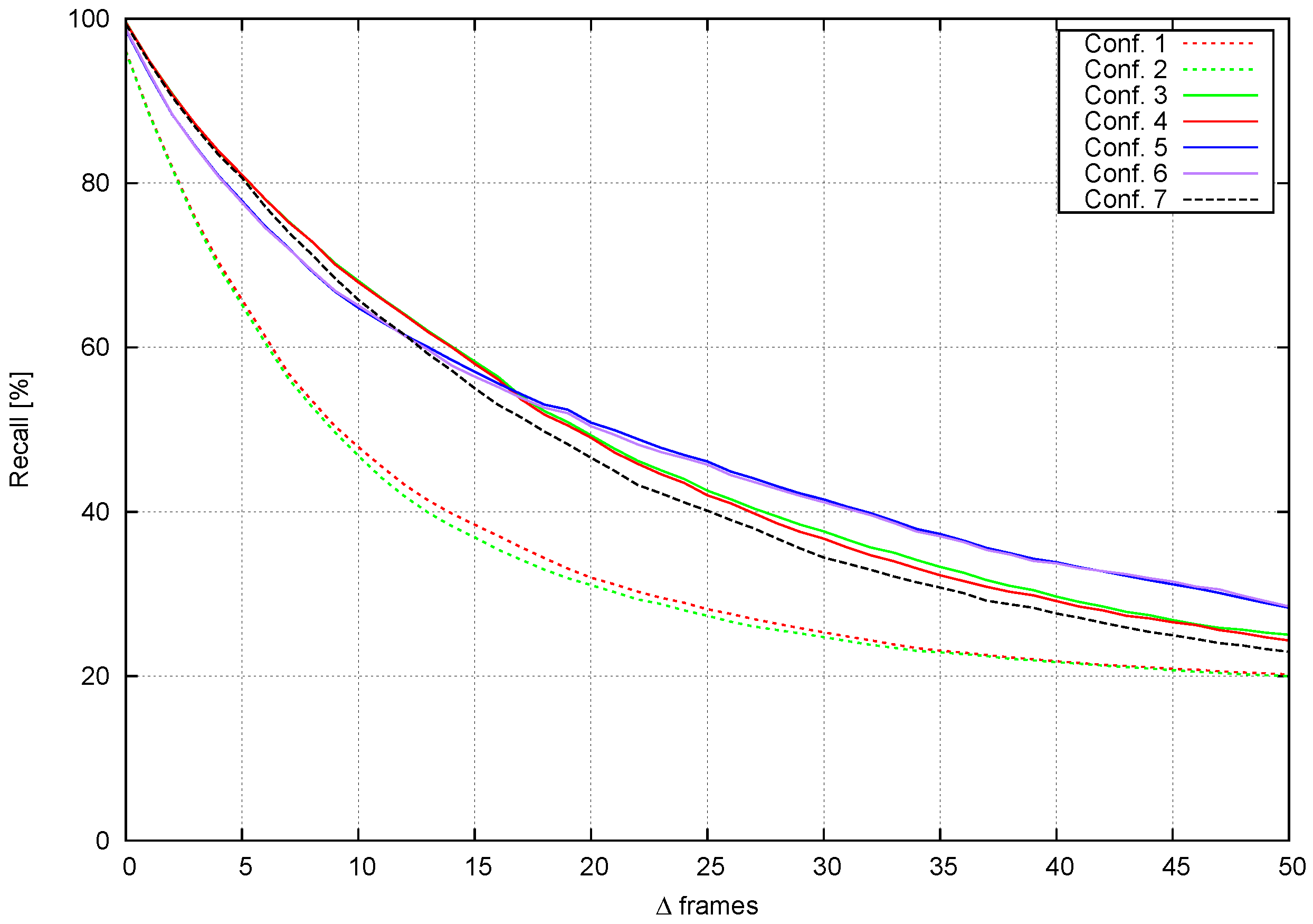
- How well tracks are recalled under various conditions.
- Computational time.
4.1. Clustering
4.2. Stixel Accuracy
4.3. Tracking
4.3.1. Sequence Performance
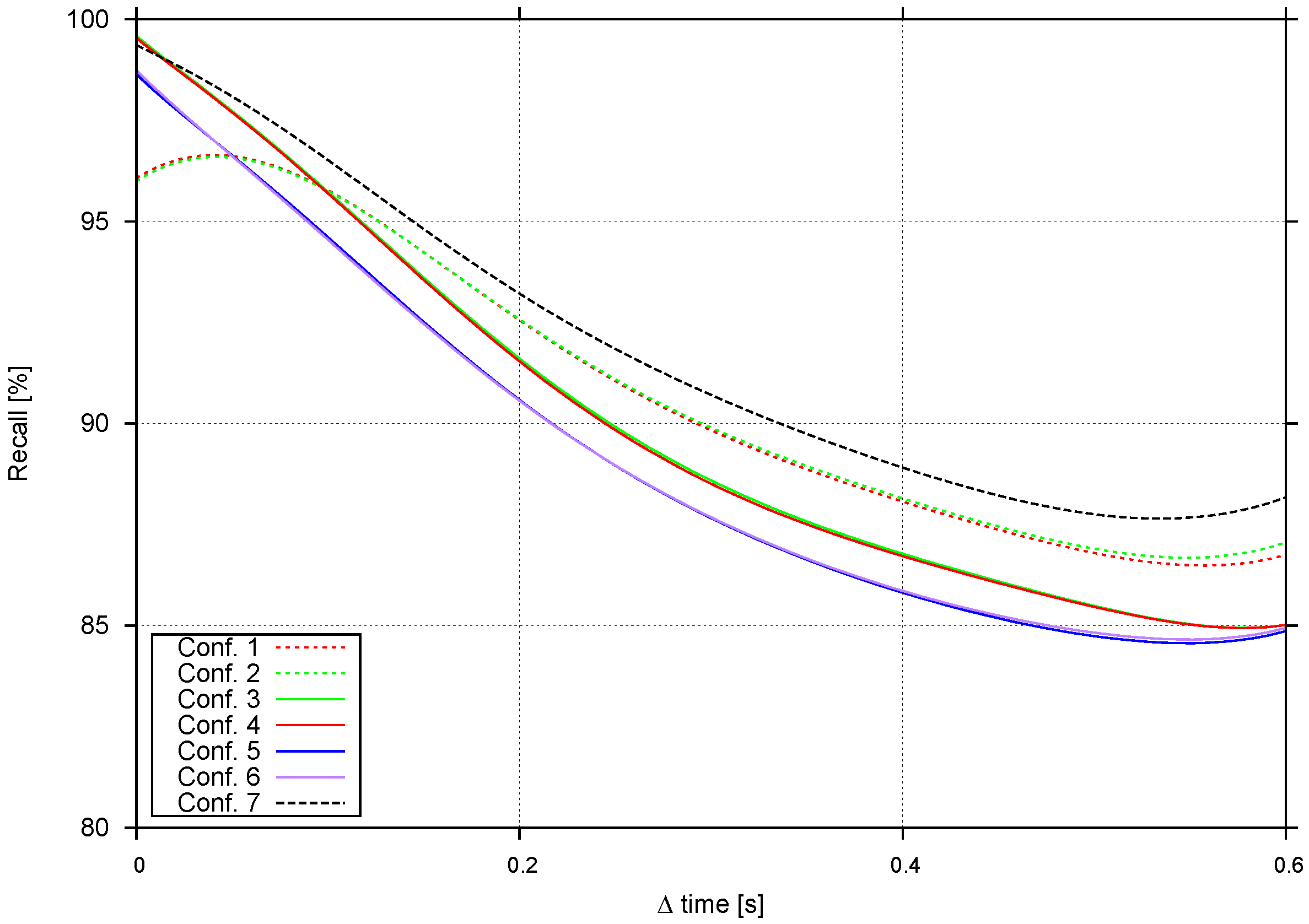
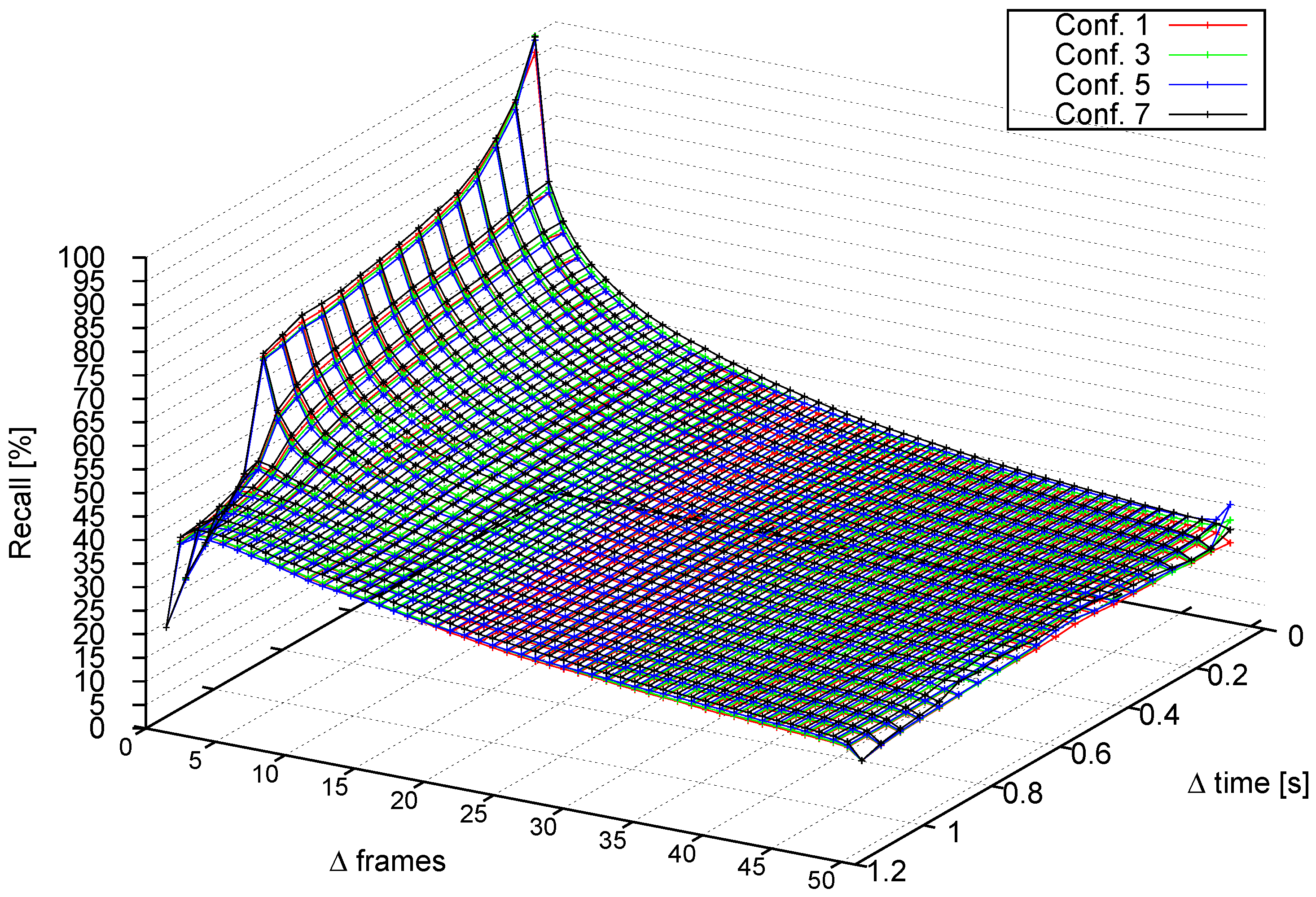
4.3.2. Performance at Different Frame Rates
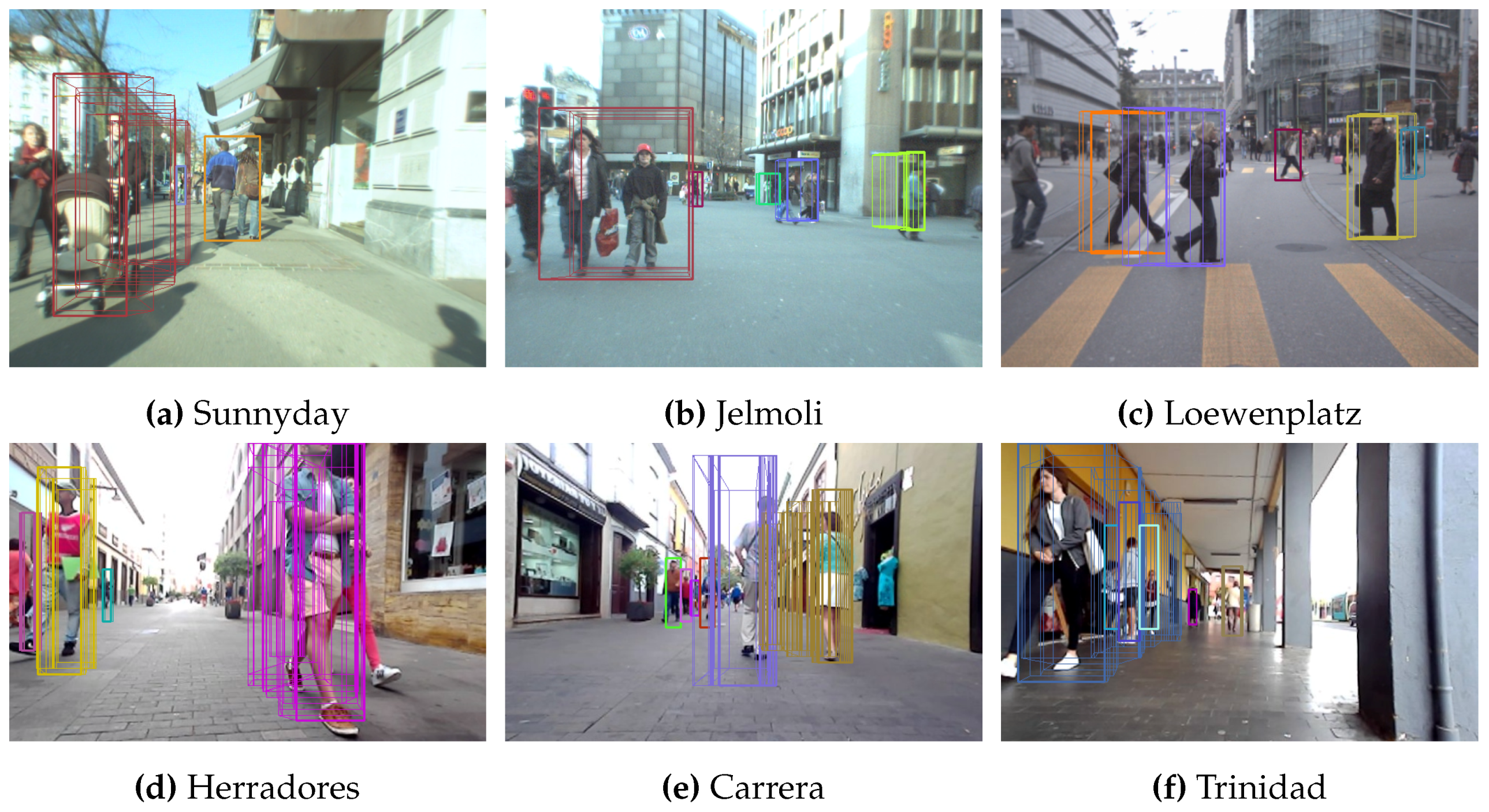
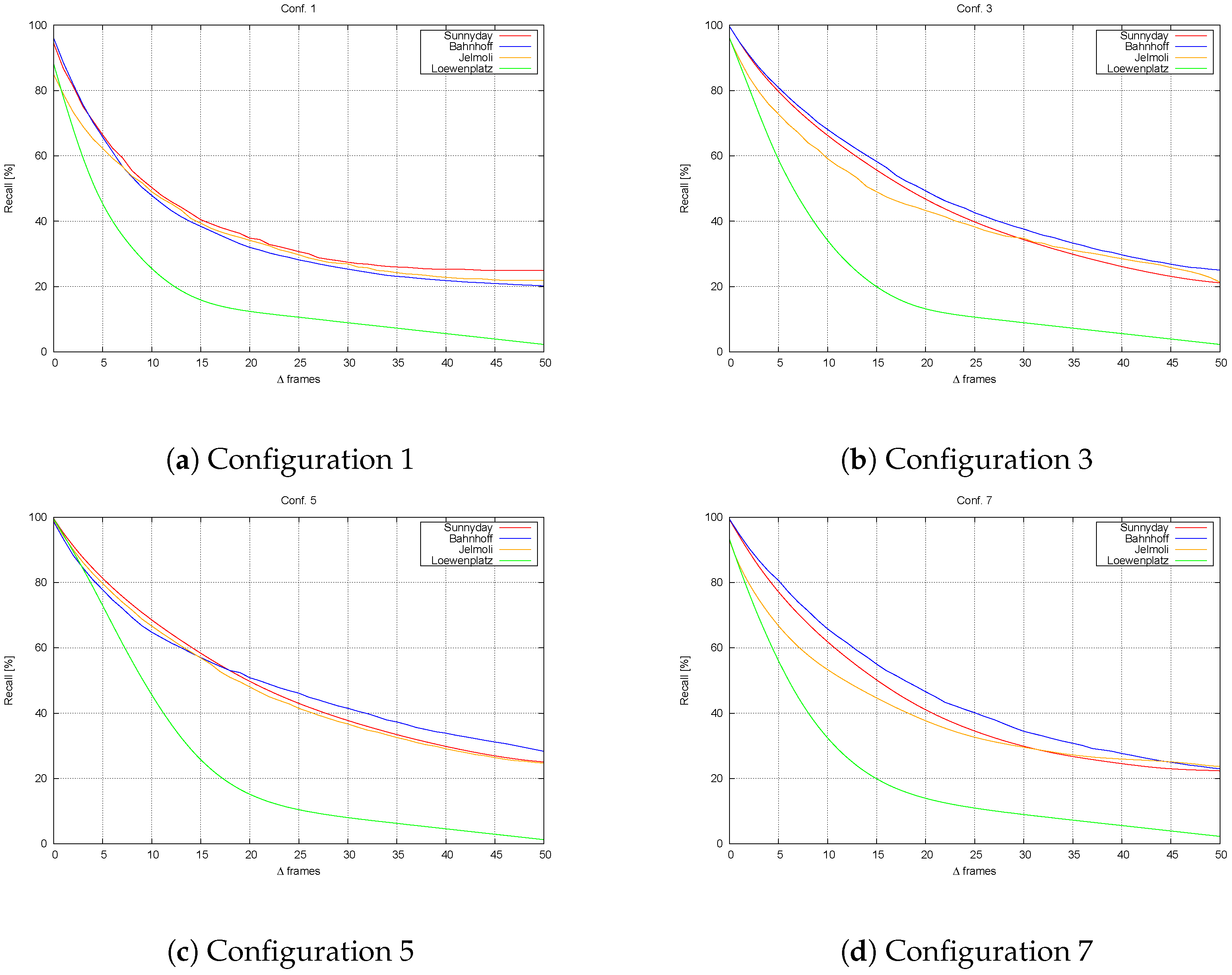
4.3.3. Performance with Other Sequences
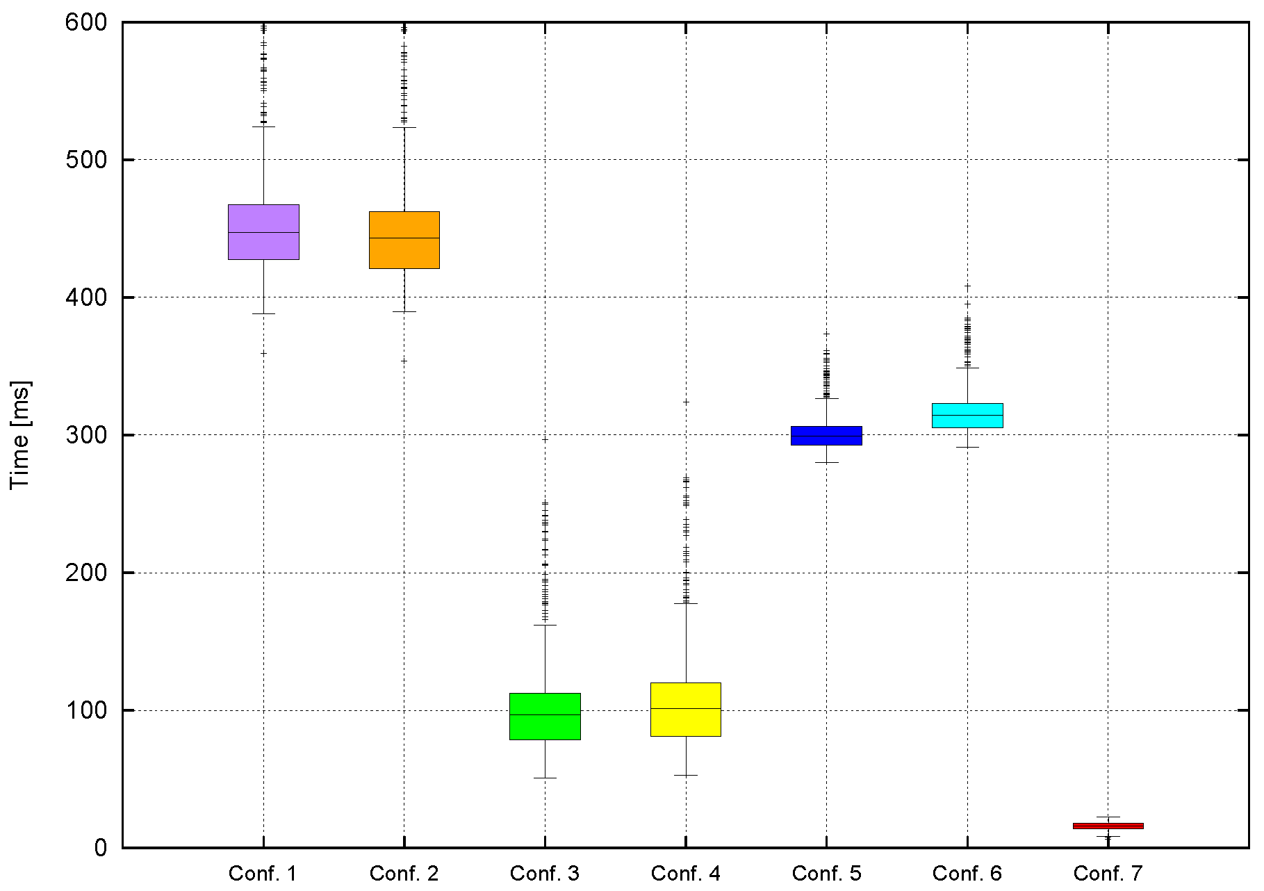
4.4. Computation Time
5. Conclusions
Supplementary Materials
Acknowledgments
Author Contributions
Conflicts of Interest
Abbreviations
| ADAS | Advanced Driver Assistance Systems |
| LIDAR | Light-Detection And Ranging |
| ROI | Region Of Interest |
References
- Badino, H.; Franke, U.; Pfeiffer, D. The stixel world —A compact medium level representation of the 3D-world. In Pattern Recognition; Springer: Berlin/Heidelberg, Germany, 2009. [Google Scholar]
- Benenson, R.; Mathias, M.; Timofte, R.; van Gool, L. Pedestrian detection at 100 frames per second. In Proceedings of the 2012 IEEE Conference on Computer Vision and Pattern Recognition, Providence, RI, USA, 16–21 June 2012; pp. 2903–2910.
- Pfeiffer, D.; Franke, U. Efficient representation of traffic scenes by means of dynamic stixels. In Proceedings of the 2010 IEEE Intelligent Vehicles Symposium, San Diego, CA, USA, 21–24 June 2010; pp. 217–224.
- VERDINO Research Project. Available online: http://verdino.webs.ull.es (accessed on 26 July 2016).
- Morales, N.; Toledo, J.T.; Acosta, L.; Arnay, R. Real-time adaptive obstacle detection based on an image database. Comput. Vis. Image Underst. 2011, 115, 1273–1287. [Google Scholar] [CrossRef]
- Perea, D.; Hernandez-Aceituno, J.; Morell, A.; Toledo, J.; Hamilton, A.; Acosta, L. MCL with sensor fusion based on a weighting mechanism versus a particle generation approach. In Proceedings of the 16th International IEEE Conference on Intelligent Transportation Systems (ITSC 2013), The Hague, The Netherlands, 6–9 October 2013; pp. 166–171.
- Gunyel, B.; Benenson, R.; Timofte, R.; van Gool, L. Stixels motion estimation without optical flow computation. Comput.Vis. 2012, 7577, 528–539. [Google Scholar]
- Sivaraman, S.; Trivedi, M.M. Looking at vehicles on the road: A survey of vision-based vehicle detection, tracking, and behavior analysis. IEEE Trans. Intell. Transp. Syst. 2013, 14, 1773–1795. [Google Scholar] [CrossRef]
- Olivares-Mendez, M.A.; Sanchez-Lopez, J.L.; Jimenez, F.; Campoy, P.; Sajadi-Alamdari, S.A.; Voos, H. Vision-based steering control, speed assistance and localization for inner-city vehicles. Sensors 2016, 16. [Google Scholar] [CrossRef] [PubMed]
- Keller, C.; Gavrila, D. Will the pedestrian cross? A study on pedestrian path prediction. IEEE Trans. Intell. Transp. Syst. 2014, 15, 494–506. [Google Scholar] [CrossRef]
- Flohr, F.; Dumitru-Guzu, M.; Kooij, J.; Gavrila, D. A probabilistic framework for joint pedestrian head and body orientation estimation. IEEE Trans. Intell. Transp. Syst. 2015, 16, 1872–1882. [Google Scholar] [CrossRef]
- Rabe, C.; Müller, T.; Wedel, A.; Franke, U. Dense, robust, and accurate motion field estimation from stereo image sequences in real-time. In Computer Vision—ECCV 2010; Springer: Berlin/Heidelberg, Germany, 2010; pp. 582–595. [Google Scholar]
- Barth, A.; Franke, U. Estimating the driving state of oncoming vehicles from a moving platform using stereo vision. IEEE Trans. Intell. Transp. Syst. 2009, 10, 560–571. [Google Scholar] [CrossRef]
- Danescu, R.; Pantilie, C.; Oniga, F.; Nedevschi, S. Particle grid tracking system stereovision based obstacle perception in driving environments. IEEE Intell. Transp. Syst. Mag. 2012, 4, 6–20. [Google Scholar] [CrossRef]
- Schauwecker, K.; Zell, A. Robust and efficient volumetric occupancy mapping with an application to stereo vision. In Proceedings of the 2014 IEEE International Conference on Robotics and Automation (ICRA), Hong Kong, China, 31 May–7 June 2014; pp. 6102–6107.
- Wurm, K.M.; Hornung, A.; Bennewitz, M.; Stachniss, C.; Burgard, W. OctoMap: A probabilistic, flexible, and compact 3D map representation for robotic systems. In Proceedings of the ICRA 2010 Workshop on Best Practice in 3D Perception and Modeling for Mobile Manipulation, Anchorage, AK, USA, 7 May 2010.
- Broggi, A.; Cattani, S.; Patander, M.; Sabbatelli, M.; Zani, P. A full-3D voxel-based dynamic obstacle detection for urban scenario using stereo vision. In Proceedings of the 16th International IEEE Conference on Intelligent Transportation Systems (ITSC 2013), The Hague, The Netherlands, 6–9 October 2013; pp. 71–76.
- Yu, Y.; Li, J.; Guan, H.; Wang, C. Automated extraction of urban road facilities using mobile laser scanning data. IEEE Trans. Intell. Transp. Syst. 2015, 16, 2167–2181. [Google Scholar] [CrossRef]
- Fotiadis, E.P.; Garzón, M.; Barrientos, A. Human detection from a mobile robot using fusion of laser and vision information. Sensors 2013, 13, 11603–11635. [Google Scholar] [CrossRef] [PubMed]
- González, A.; Fang, Z.; Socarras, Y.; Serrat, J.; Vázquez, D.; Xu, J.; López, A.M. Pedestrian detection at day/night time with visible and FIR cameras: A comparison. Sensors 2016, 16. [Google Scholar] [CrossRef] [PubMed]
- Zhang, L.; Li, Y.; Nevatia, R. Global data association for multi-object tracking using network flows. In Proceedings of the IEEE Conference on Computer Vision and Pattern Recognition, Anchorage, AK, USA, 23–28 June 2008; pp. 1–8.
- Henschel, R.; Leal-Taixé, L.; Rosenhahn, B. Efficient multiple people tracking using minimum cost arborescences. In Pattern Recognition; Springer International Publishing: Cham, Switzerland, 2014; pp. 265–276. [Google Scholar]
- Li, W.; Song, D. Featureless motion vector-based simultaneous localization, planar surface extraction, and moving obstacle tracking. In Algorithmic Foundations of Robotics XI; Springer International Publishing: Cham, Switzerland, 2015; pp. 245–261. [Google Scholar]
- Vatavu, A.; Danescu, R.; Nedevschi, S. Stereovision-based multiple object tracking in traffic scenarios using free-form obstacle delimiters and particle filters. IEEE Trans. Intell. Transp. Syst. 2015, 16, 498–511. [Google Scholar] [CrossRef]
- Kassir, M.M.; Palhang, M. A region based CAMShift tracking with a moving camera. In Proceedings of the 2014 Second RSI/ISM International Conference on Robotics and Mechatronics (ICRoM), Tehran, Iran, 15–17 October 2014; pp. 451–455.
- Ess, A.; Leibe, B.; Schindler, K.; van Gool, L. Robust multiperson tracking from a mobile platform. IEEE Trans. Pattern Anal. Mach. Intell. 2009, 31, 1831–1846. [Google Scholar] [CrossRef] [PubMed]
- Leal-Taixé, L.; Pons-Moll, G.; Rosenhahn, B. Everybody needs somebody: Modeling social and grouping behavior on a linear programming multiple people tracker. In Proceedings of the2011 IEEE International Conference on Computer Vision Workshops (ICCV Workshops), Barcelona, Spain, 6–13 November 2011; pp. 120–127.
- Leal-Taixé, L.; Fenzi, M.; Kuznetsova, A.; Rosenhahn, B.; Savarese, S. Learning an image-based motion context for multiple people tracking. In Proceedings of the 2014 IEEE Conference on Computer Vision and Pattern Recognition (CVPR), Columbus, OH, USA, 23–28 June 2014; pp. 3542–3549.
- Pellegrini, S.; Ess, A.; Schindler, K.; van Gool, L. You’ll never walk alone: Modeling social behavior for multi-target tracking. In Proceedings of the 2009 IEEE 12th International Conference on Computer Vision 2009, Kyoto, Japan, 29 September–2 October 2009; pp. 261–268.
- Davey, S.J.; Vu, H.X.; Arulampalam, S.; Fletcher, F.; Lim, C.C. Histogram probabilistic multi-hypothesis tracker with colour attributes. IET Radar Sonar Navig. 2015, 9, 999–1008. [Google Scholar] [CrossRef]
- Bar-Shalom, Y.; Daum, F.; Huang, J. The probabilistic data association filter. IEEE Control Syst. 2009, 29, 82–100. [Google Scholar] [CrossRef]
- Scharwächter, T.; Enzweiler, M.; Franke, U.; Roth, S. Stixmantics: A medium-level model for real-time semantic scene understanding. In Computer Vision—ECCV 2014; Springer International Publishing: Cham, Switzerland, 2014; pp. 533–548. [Google Scholar]
- Benenson, R.; Mathias, M.; Timofte, R.; van Gool, L. Fast stixel computation for fast pedestrian detection. In Computer Vision—ECCV 2014; Springer: Berlin/Heidelberg, Germany, 2012; pp. 11–20. [Google Scholar]
- Pfeiffer, D.; Franke, U.; Daimler, A.G. Towards a Global Optimal Multi-Layer Stixel Representation of Dense 3D Data; BMVA Press: Dundee, UK, 2011; pp. 1–12. [Google Scholar]
- Pfeiffer, D.; Gehrig, S.; Schneider, N. Exploiting the power of stereo confidences. In Proceedings of the 2013 IEEE Conference on Computer Vision and Pattern Recognition, Portland, OR, USA, 23–28 June 2013; pp. 297–304.
- Muffert, M.; Milbich, T.; Pfeiffer, D.; Franke, U. May I enter the roundabout? A time-to-contact computation based on stereo-vision. In Proceedings of the 2012 IEEE Intelligent Vehicles Symposium, Alcala de Henares, Spain, 3–7 June 2012; pp. 565–570.
- Benenson, R.; Timofte, R.; van Gool, L. Stixels estimation without depth map computation. In Proceedings of the 2011 IEEE International Conference on Computer Vision Workshops (ICCV Workshops), Barcelona, Spain, 6–13 November 2011; pp. 2010–2017.
- Chung, J.; Kannappan, P.; Ng, C.; Sahoo, P. Measures of distance between probability distributions. J. Math. Anal. Appl. 1989, 138, 280–292. [Google Scholar] [CrossRef]
- Edmonds, J. Paths, trees, and flowers. Can. J. Math. 1965, 17, 449–467. [Google Scholar] [CrossRef]
- Pollefeys, M.; Koch, R.; van Gool, L. A simple and efficient rectification method for general motion. In Proceedings of the Proceedings of the Seventh IEEE International Conference on Computer Vision, Kerkyra, Greece, 20 –27 September 1999; pp. 496–501.
- Luong, Q.T.; Faugeras, O.D. The fundamental matrix: Theory, algorithms, and stability analysis. Int. J. Comput. Vis. 1996, 17, 43–75. [Google Scholar] [CrossRef]
- Chu, K.; Lee, M.; Sunwoo, M. Local path planning for off-road autonomous driving with avoidance of static obstacles. IEEE Trans. Intell. Transp. Syst. 2012, 13, 1599–1616. [Google Scholar] [CrossRef]
- Arnay, R.; Morales, N.; Morell, A.; Hernandez-Aceituno, J.; Perea, D.; Toledo, J.T.; Hamilton, A.; Sanchez-Medina, J.J.; Acosta, L. Safe and reliable path planning for the autonomous vehicle verdino. IEEE Intell. Transp. Syst. Mag. 2016, 8, 22–32. [Google Scholar] [CrossRef]
- Morales, N.; Arnay, R.; Toledo, J.; Morell, A.; Acosta, L. Safe and reliable navigation in crowded unstructured pedestrian areas. Eng. Appl. Art. Intell. 2016, 49, 74–87. [Google Scholar] [CrossRef]
- Morales, N.; Toledo, J.; Acosta, L. Generating automatic road network definition files for unstructured areas using a multiclass support vector machine. Inf. Sci. 2016, 329, 105–124. [Google Scholar] [CrossRef]
- Morales, N.; Toledo, J.; Acosta, L. Path planning using a multiclass support vector machine. Appl. Soft Comput. 2016, 43, 498–509. [Google Scholar] [CrossRef]
- Lu, D.V.; Hershberger, D.; Smart, W.D. Layered costmaps for context-sensitive navigation. In Proceedings of the 2014 IEEE/RSJ International Conference on Intelligent Robots and Systems, Chicago, IL, USA, 14–18 September 2014; pp. 709–715.
- ROS.org. Available online: http://www.ros.org (accessed on 26 July 2016).
- Stixel_world at GitHub. Available online: https://github.com/nestormh/stixel_world (accessed on 26 July 2016).


| Configuration 1 | 1 | - | 0 | Gunyel et al. [7] |
| Configuration 2 | 0.5 | - | 0.5 | Gunyel et al. [7] |
| Configuration 3 | 1 | 0 | 0 | Two-level tracking |
| Configuration 4 | 0.5 | 0 | 0.5 | Two-level tracking |
| Configuration 5 | 0 | 1 | 0 | Two-level tracking |
| Configuration 6 | 0 | 0.5 | 0.5 | Two-level tracking |
| Configuration 7 | - | - | - | Object tracking |
© 2016 by the authors; licensee MDPI, Basel, Switzerland. This article is an open access article distributed under the terms and conditions of the Creative Commons Attribution (CC-BY) license (http://creativecommons.org/licenses/by/4.0/).
Share and Cite
Morales, N.; Morell, A.; Toledo, J.; Acosta, L. Fast Object Motion Estimation Based on Dynamic Stixels. Sensors 2016, 16, 1182. https://doi.org/10.3390/s16081182
Morales N, Morell A, Toledo J, Acosta L. Fast Object Motion Estimation Based on Dynamic Stixels. Sensors. 2016; 16(8):1182. https://doi.org/10.3390/s16081182
Chicago/Turabian StyleMorales, Néstor, Antonio Morell, Jonay Toledo, and Leopoldo Acosta. 2016. "Fast Object Motion Estimation Based on Dynamic Stixels" Sensors 16, no. 8: 1182. https://doi.org/10.3390/s16081182
APA StyleMorales, N., Morell, A., Toledo, J., & Acosta, L. (2016). Fast Object Motion Estimation Based on Dynamic Stixels. Sensors, 16(8), 1182. https://doi.org/10.3390/s16081182