
Scan Line Based Road Marking Extraction from Mobile LiDAR Point Clouds †


Abstract
:
1. Introduction
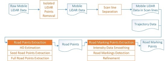
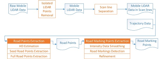
2. Preprocessing
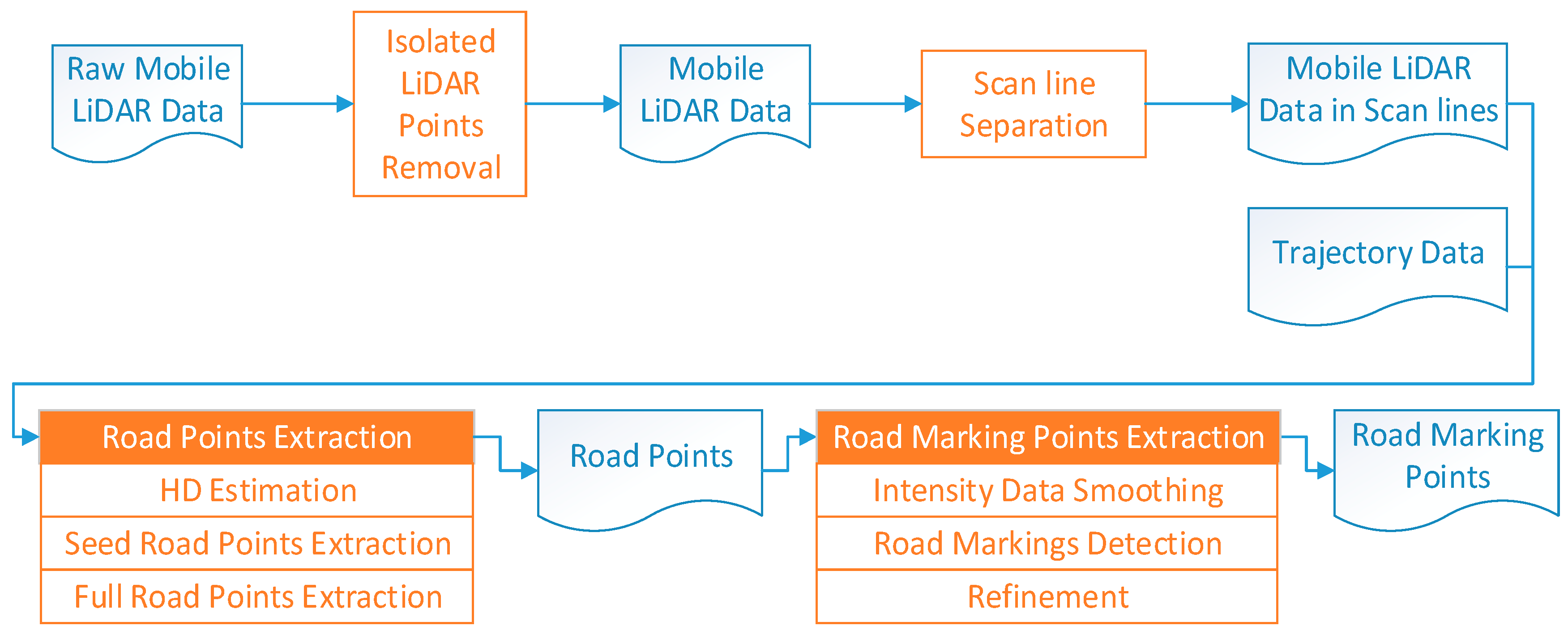
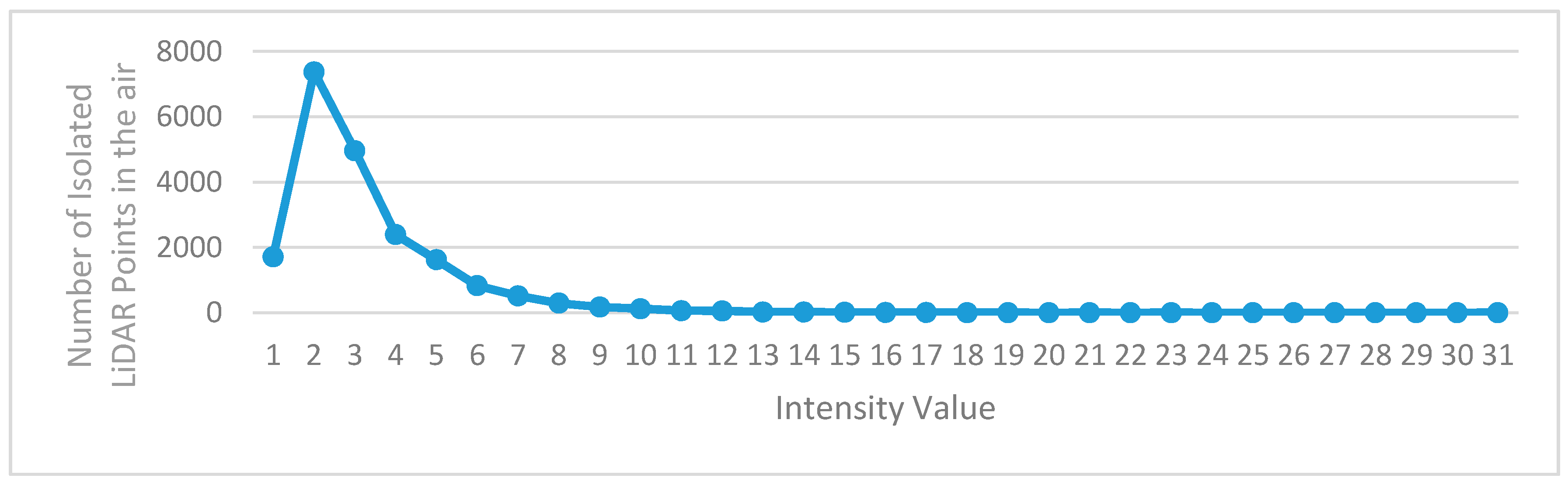
2.1. Isolated LiDAR Points Removal
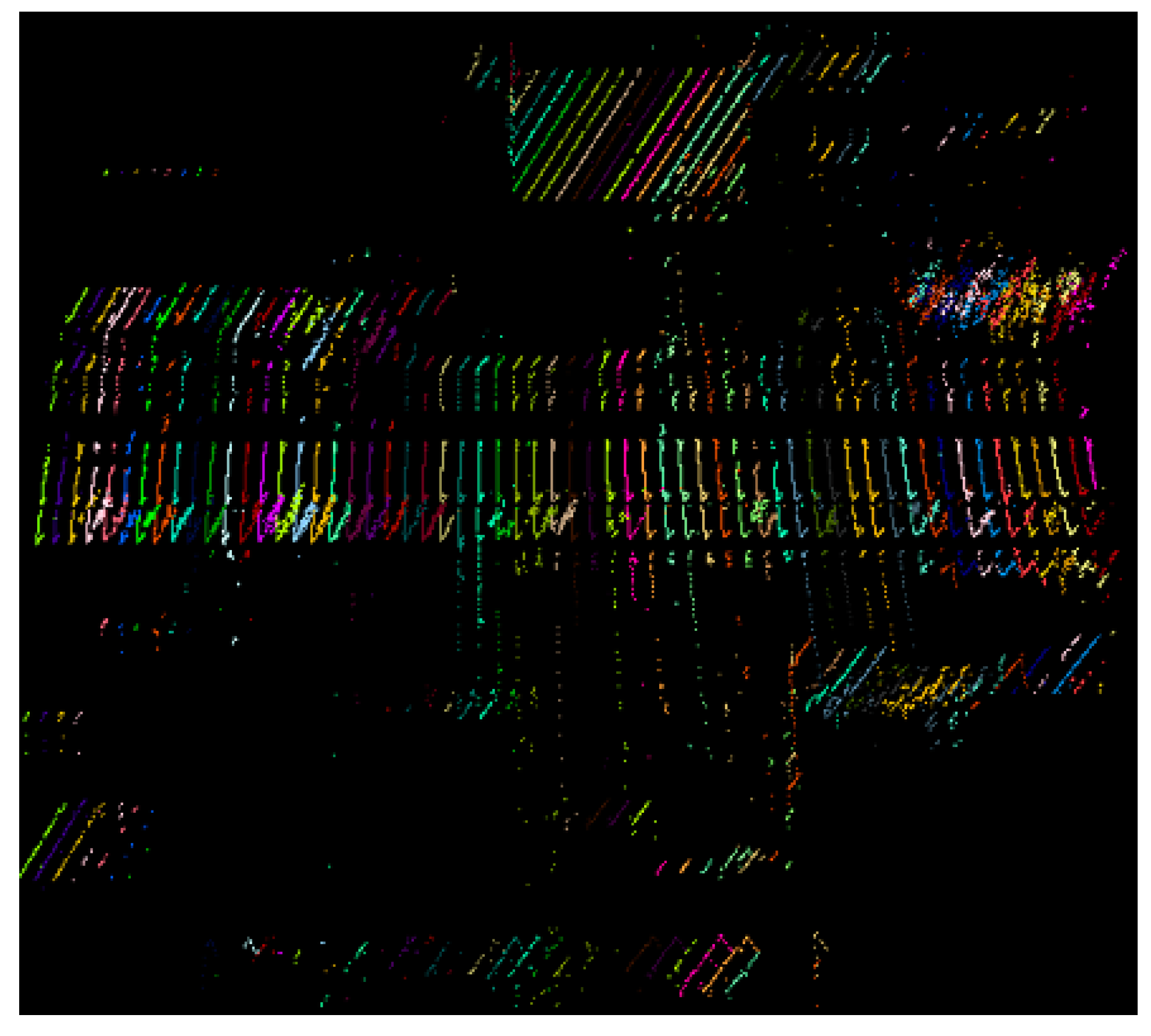
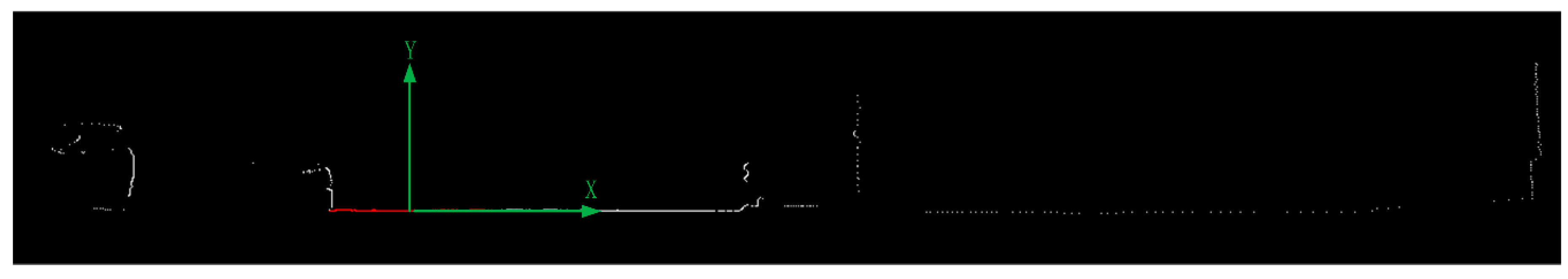
2.2. Scan Line Separation
3. Road Points Extraction
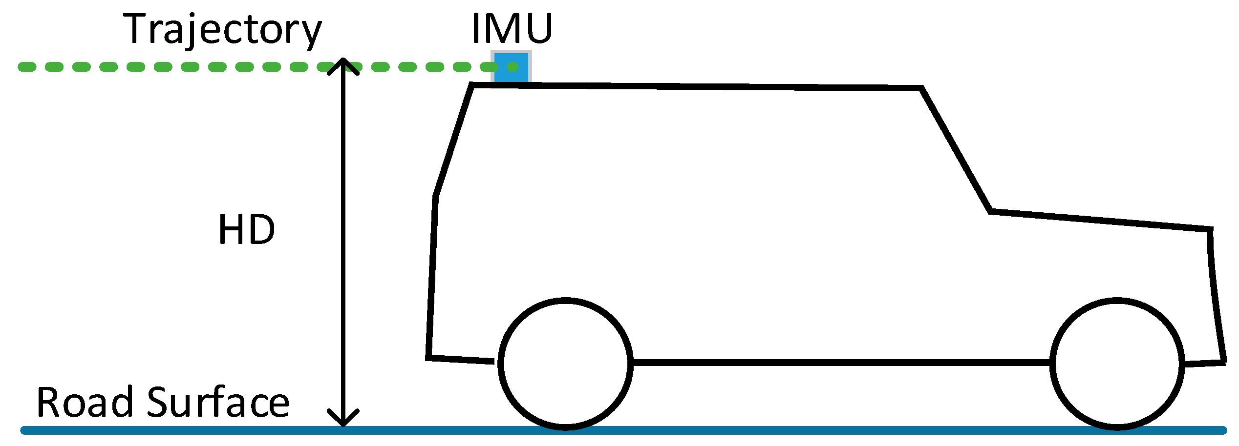
3.1. HD Estimation
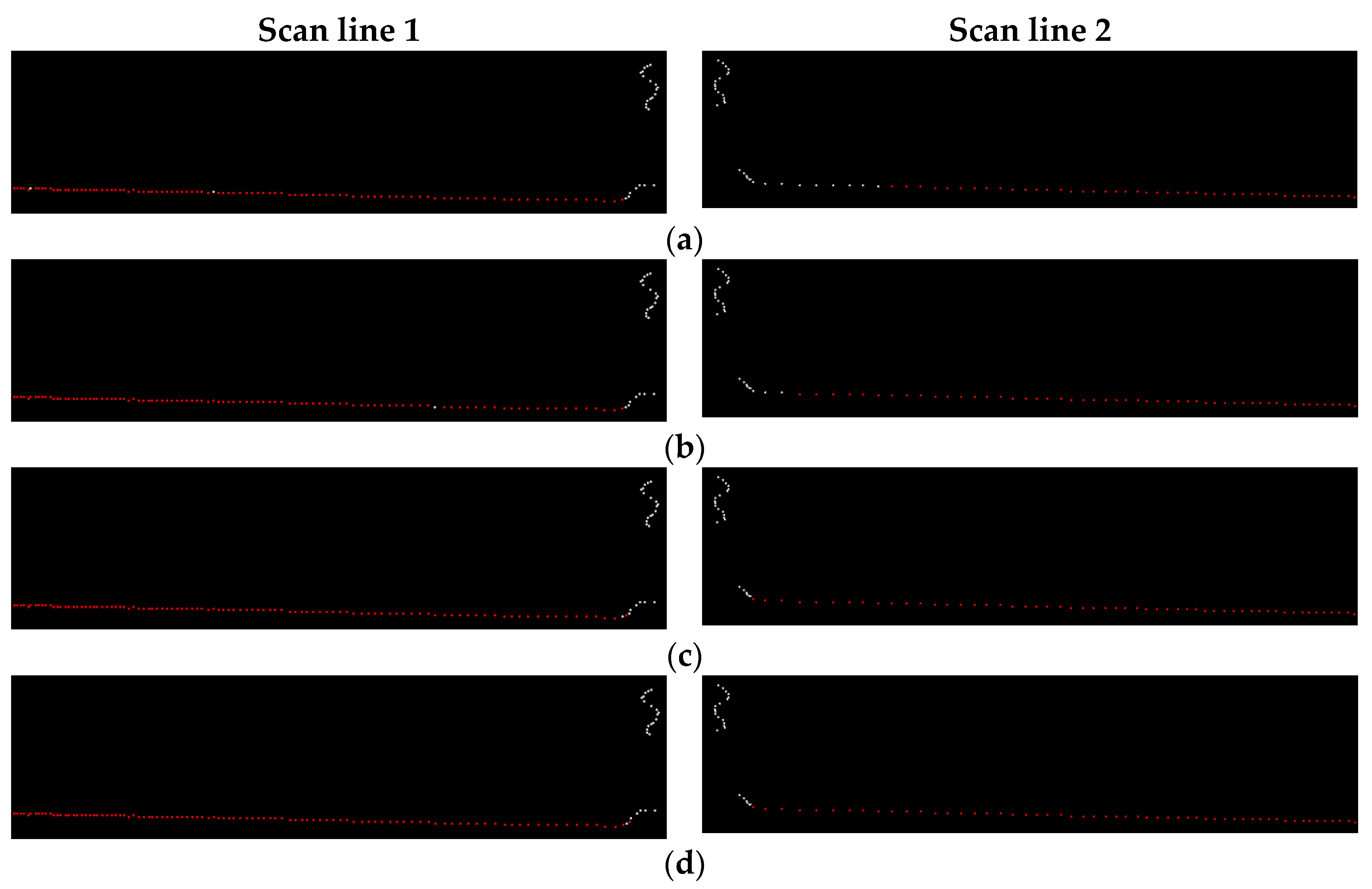
3.2. Seed Road Points Extraction from Scan Line
3.3. Full Road Points Extraction from Scan Line
4. Road Markings Extraction and Refinement
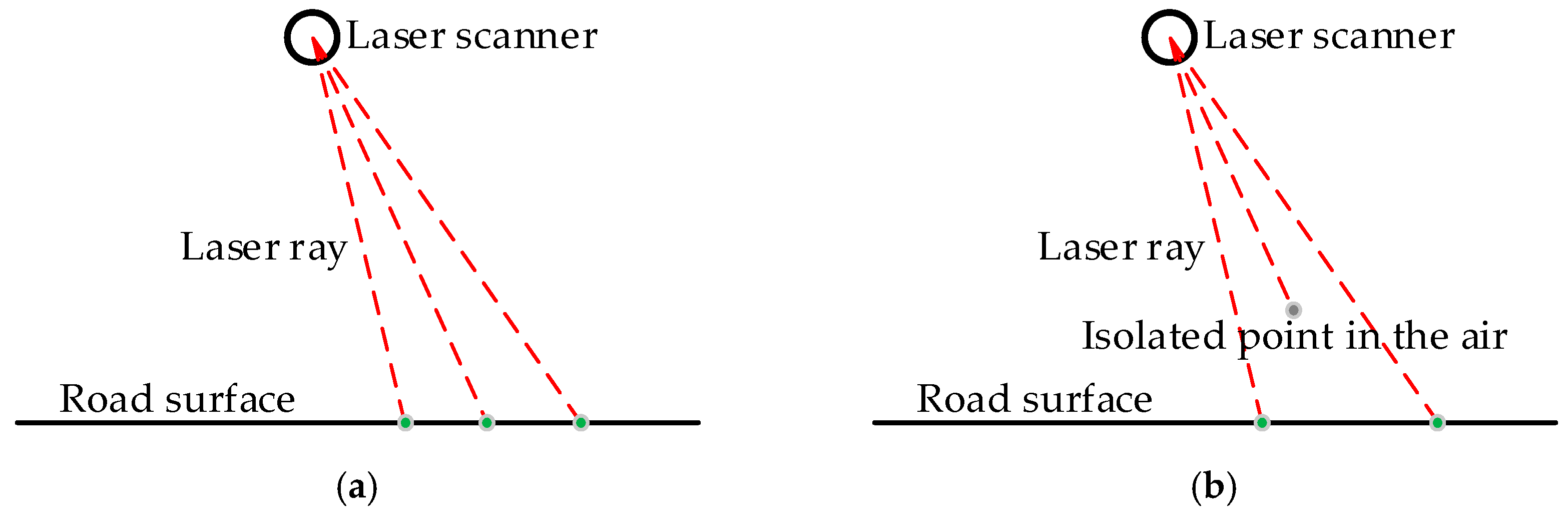
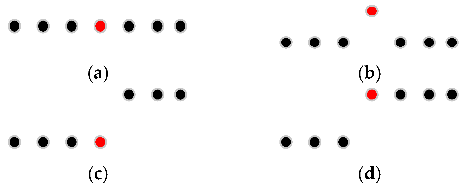
4.1. Intensity Data Smoothing by Dynamic Window Median Filter
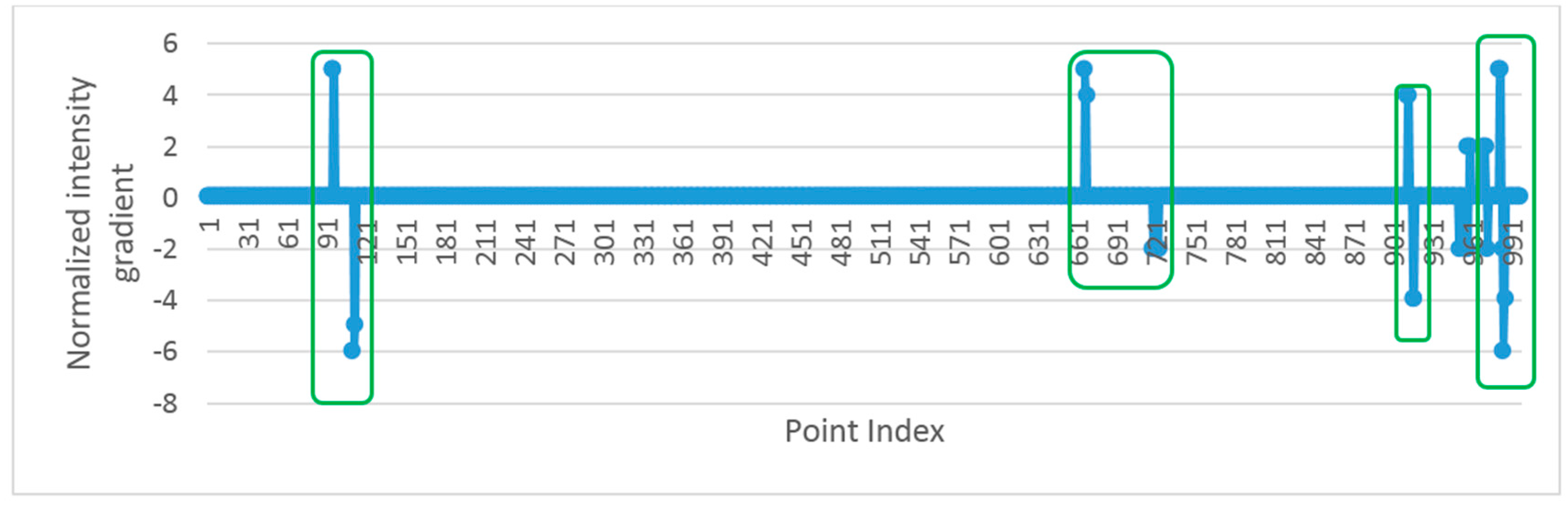
4.2. Road Markings Extraction by EDEC
4.3. Segment and Dimensionality Feature Based Refinement
5. Results and Discussion
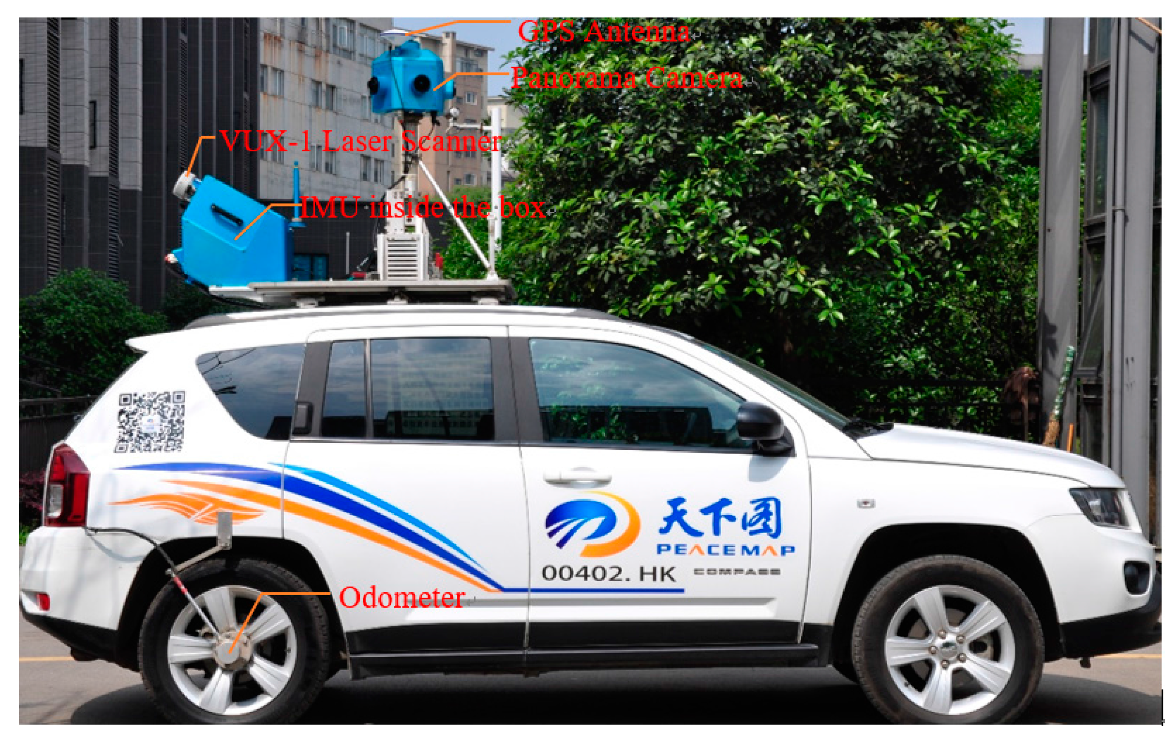
5.1. The Mobile LiDAR System and Mobile LiDAR Dataset
5.2. Parameter Sensitivity Analysis
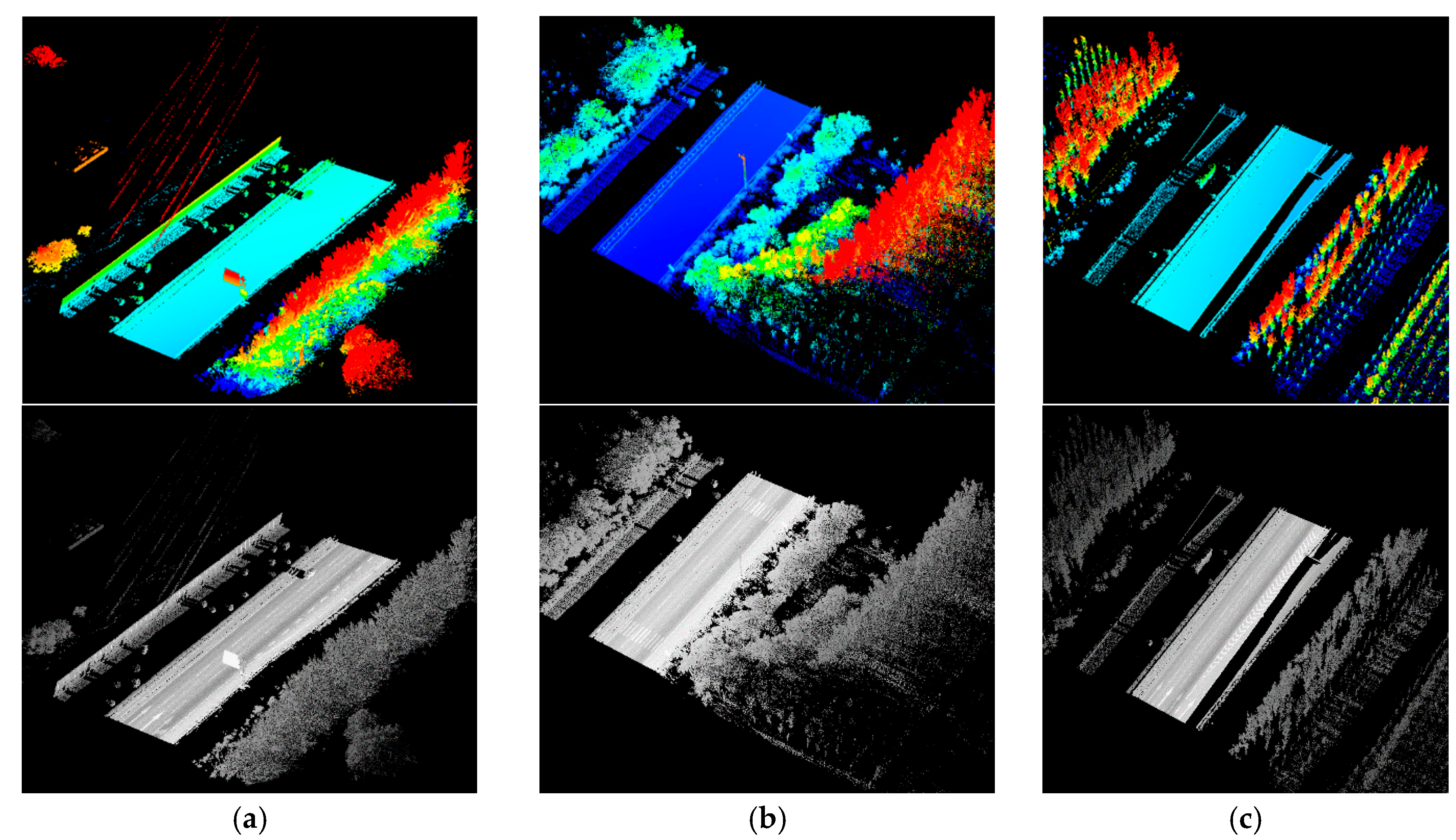
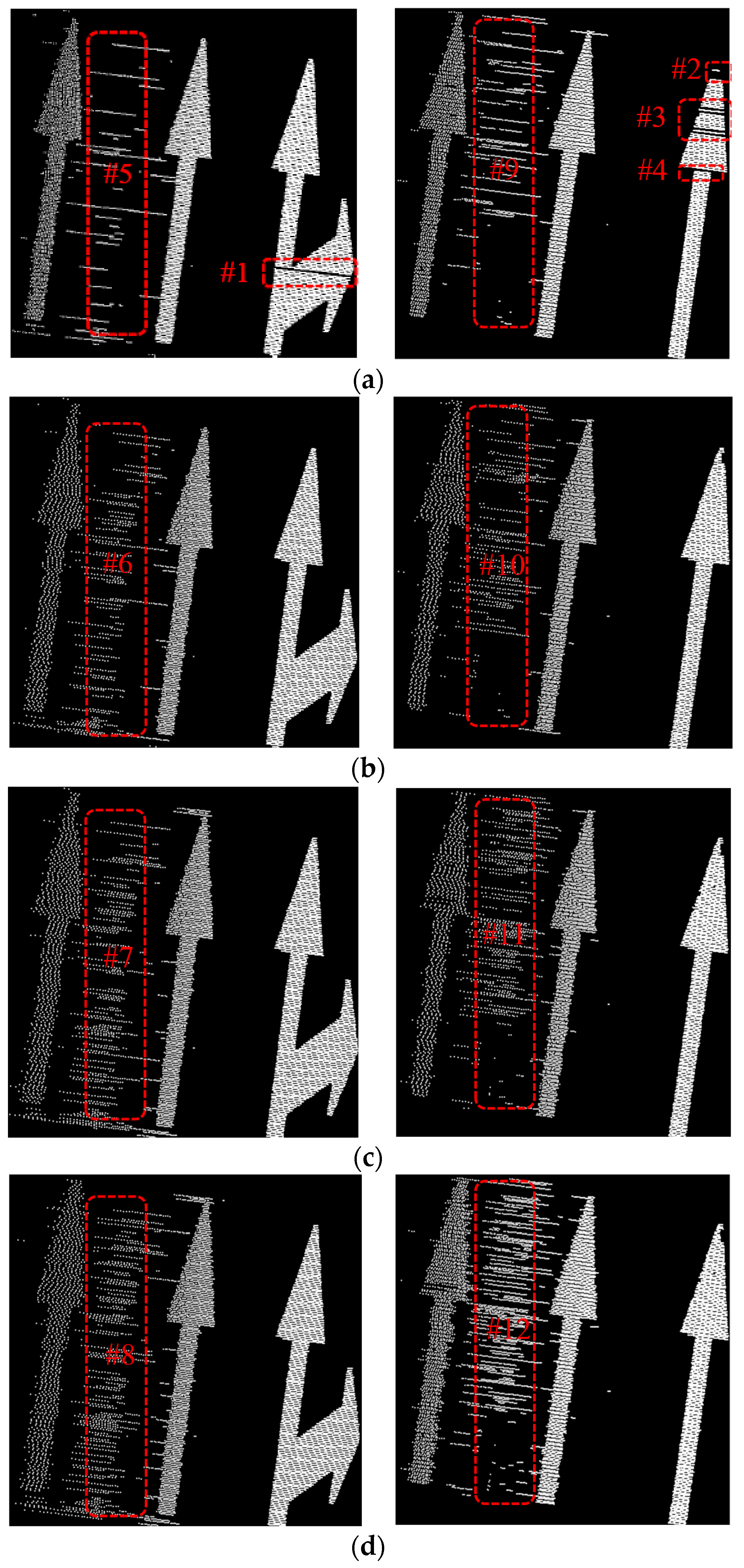
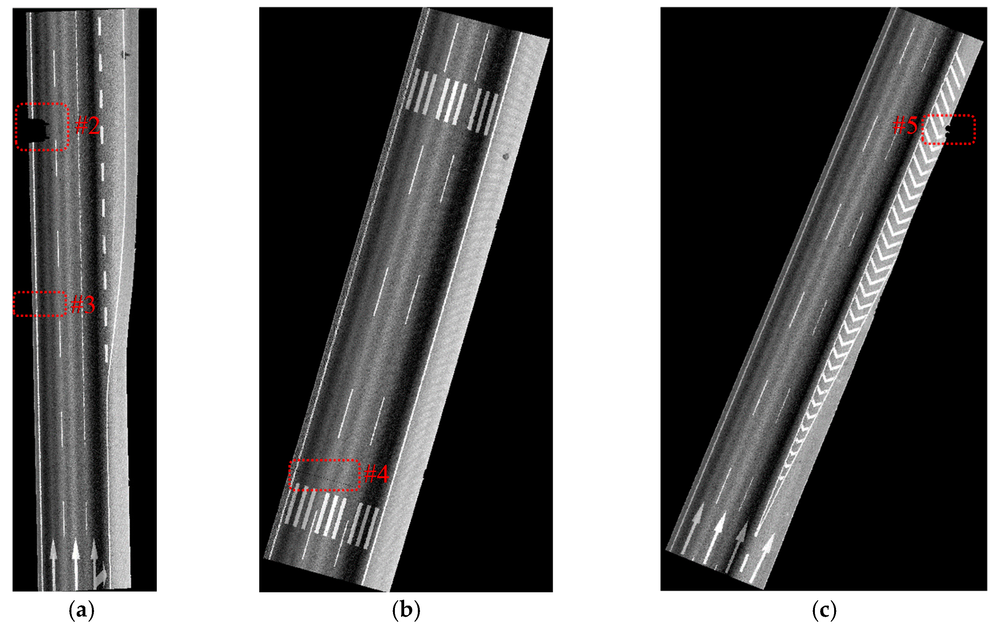
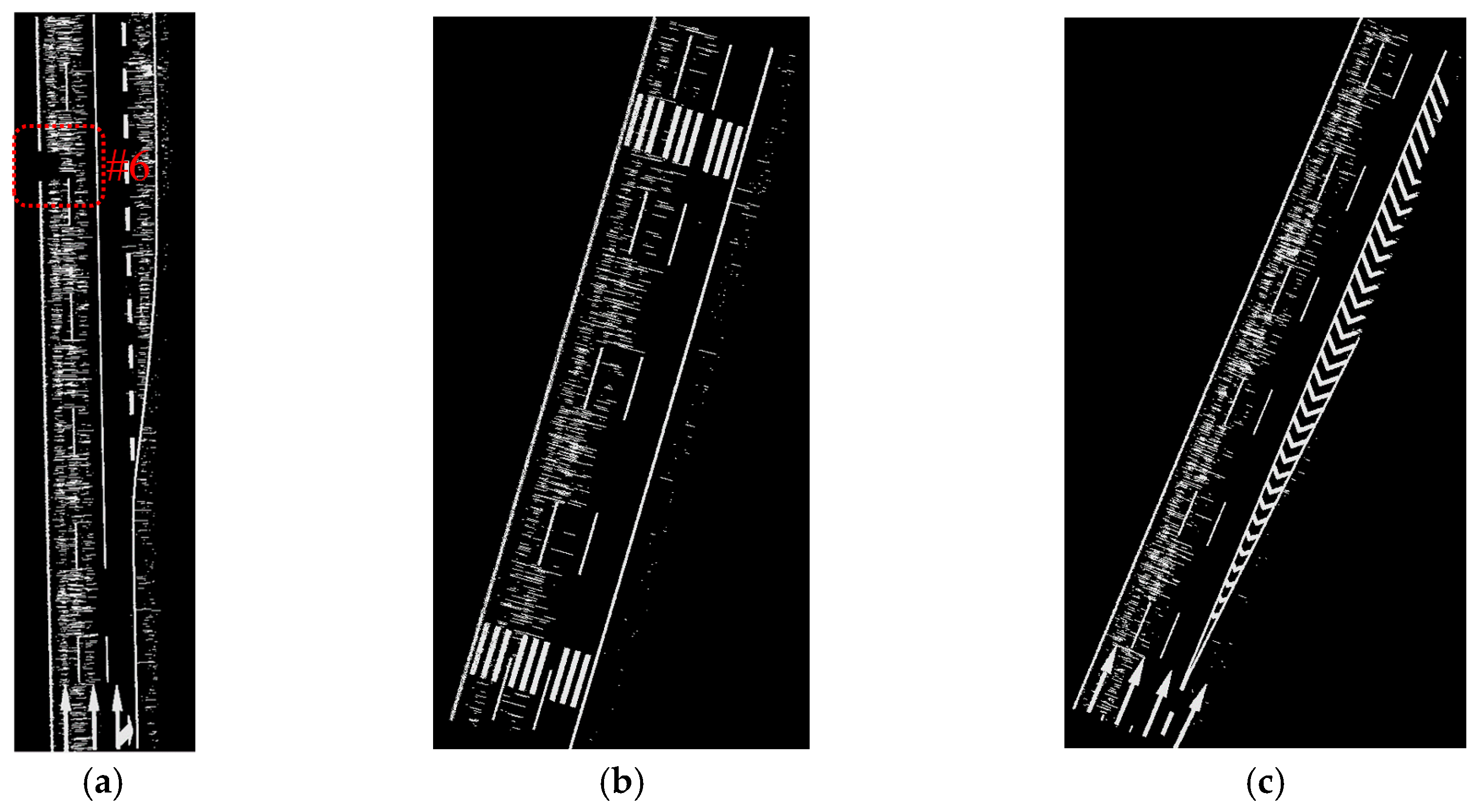
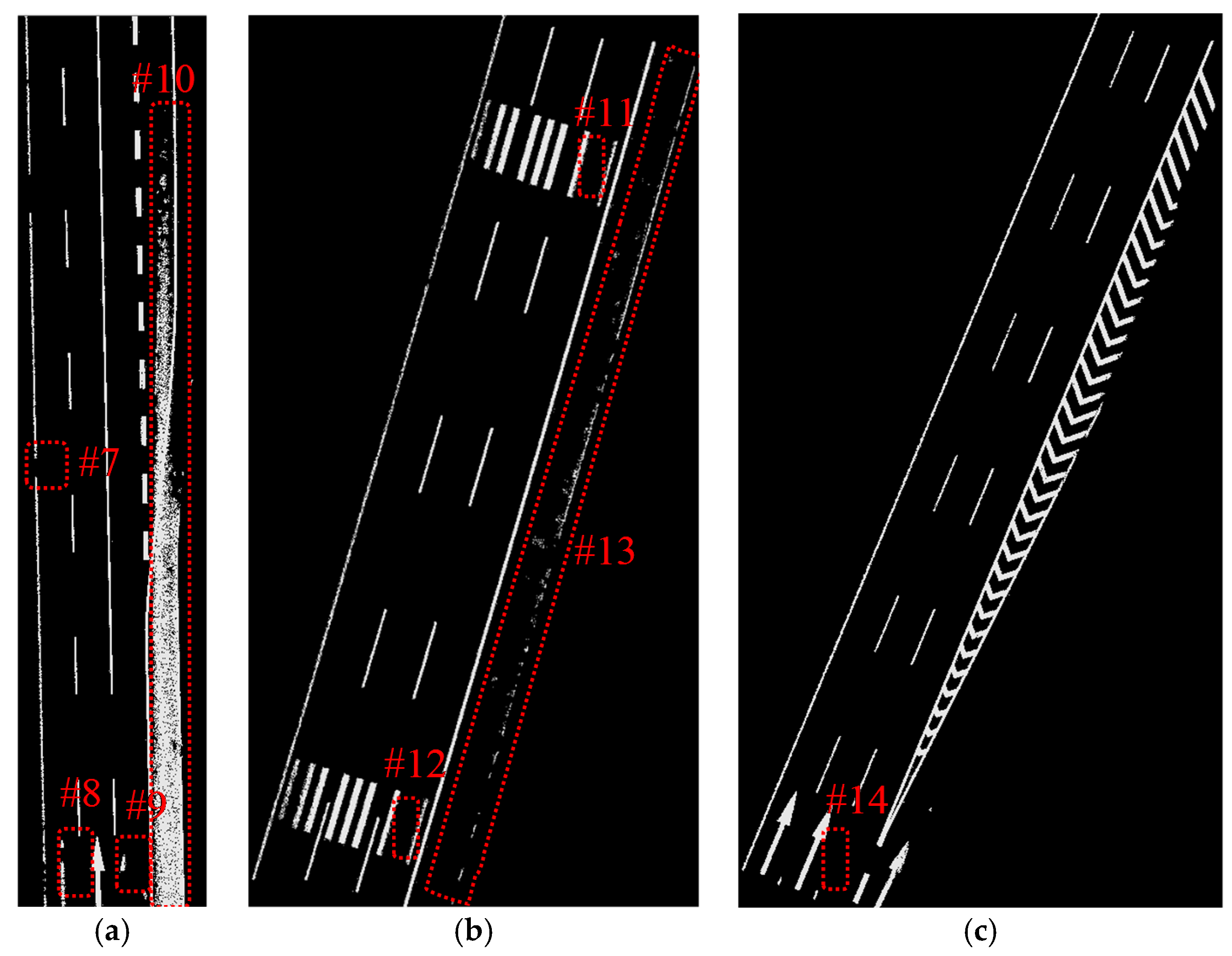
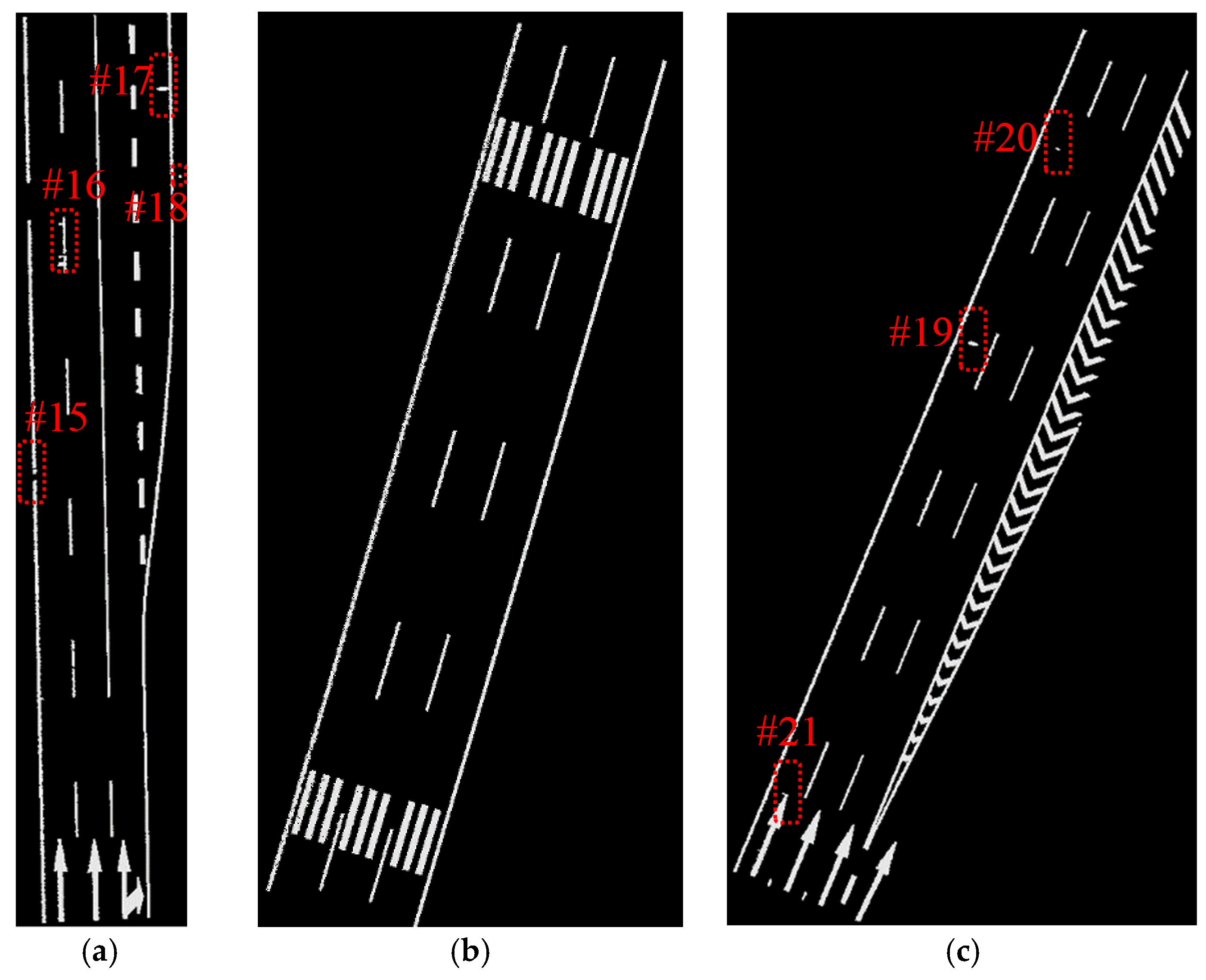
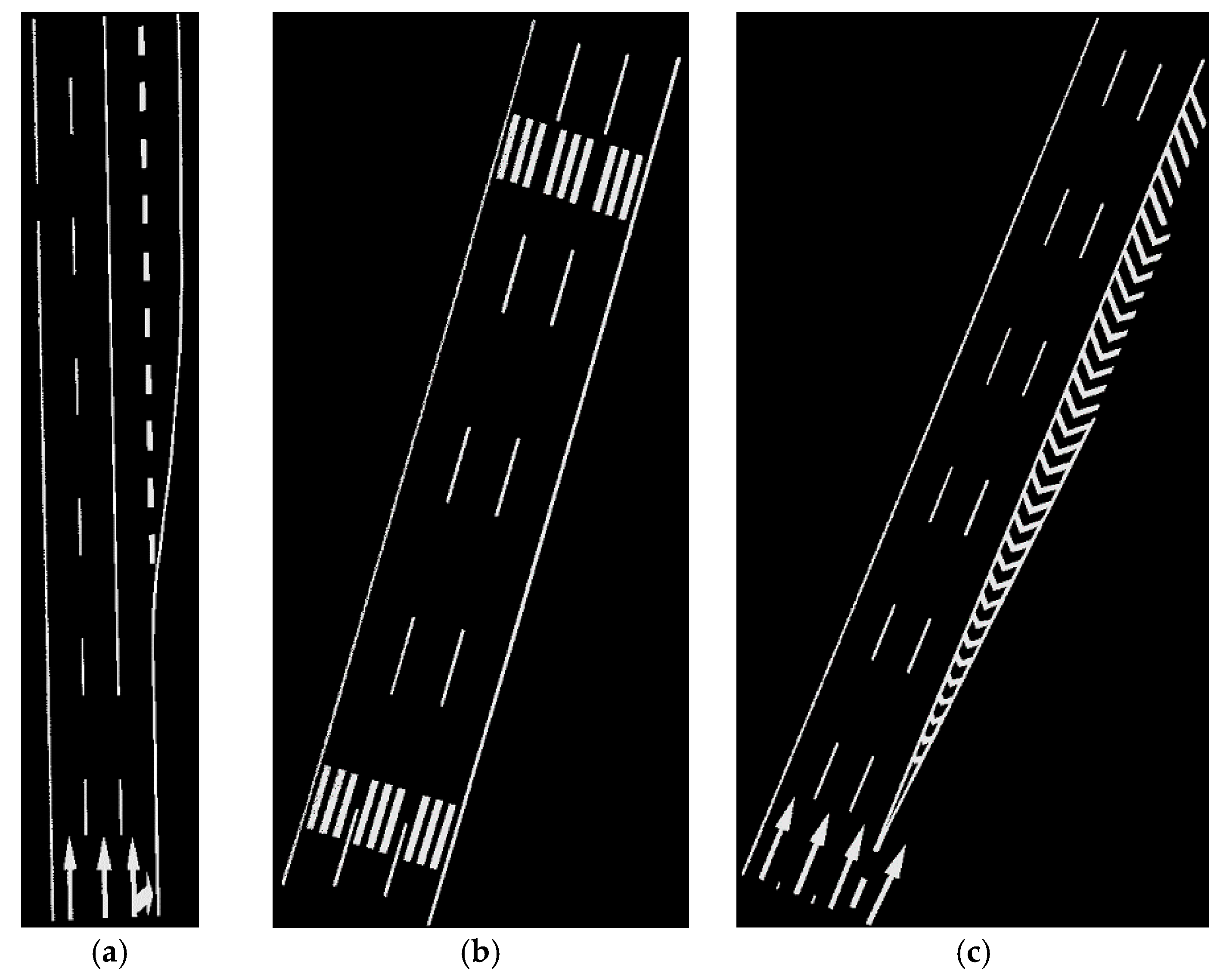
5.3. Road Points Extraction and Road Markings Extraction
6. Conclusions
Acknowledgments
Author Contributions
Conflicts of Interest
References
- Novak, K. The Ohio State University Highway Mapping System: The Stereo Vision System Component. In Proceedings of the 47th Annual Meeting of the Institute of Navigation, Williamsburg, VA, USA, 10–12 June 1991; pp. 121–124.
- Goad, C.C. The Ohio State University Highway Mapping System: The Positioning Component. In Proceedings of the 47th Annual Meeting of The Institute of Navigation, Williamsburg, VA, USA, 10–12 June 1991; pp. 117–120.
- Schwarz, K.P.; Martell, H.E.; El-Sheimy, N.; Li, R.; Chapman, M.A.; Cosandier, D. VIASAT—A Mobile Highway Survey System of High Accuracy. In Proceedings of the Vehicle Navigation and Information Systems Conference, Ottawa, ON, Canada, 12–15 October 1993; pp. 476–481.
- El-Sheimy, N.; Schwarz, K.P. Kinematic Positioning in Three Dimensions Using CCD Technology. In Proceedings of the Institute of Electrical and Electronics Engineers Vehicle Navigation and Information Systems Conference, Ottawa, ON, Canada, 12–15 October 1993; pp. 472–475.
- Hock, C.; Caspary, W.; Heister, H.; Klemm, J.; Sternberg, H. Architecture and Design of the Kinematic Survey System KiSS. In Proceedings of the 3rd International Workshop on High Precision Navigation, Stuttgart, Germany, April 1995; pp. 569–576.
- He, G. Design and Application of the GPSVision Mobile Mapping System. Int. Arch. Photogram. Remote Sens. Spat. Inf. Sci. 2002, 34, 163–168. [Google Scholar]
- Brown, A. High Accuracy Targeting Using a GPS-Aided Inertial Measurement Unit. In Proceedings of the ION 54th Annual Meeting, Denver, CO, USA, 1–3 June 1998.
- Puente, I.; González-Jorge, H.; Martínez-Sánchez, J.; Arias, P. Review of mobile mapping and surveying technologies. Measurement 2013, 46, 2127–2145. [Google Scholar] [CrossRef]
- Zhou, L.; Vosselman, G. Mapping curbstones in airborne and mobile laser scanning data. Int. J. Appl. Earth Obs. Geoinform. 2012, 18, 293–304. [Google Scholar] [CrossRef]
- Pu, S.; Rutzinger, M.; Vosselman, G.; Oude Elberink, S. Recognizing basic structures from mobile laser scanning data for road inventory studies. ISPRS J. Photogramm. 2011, 66, S28–S39. [Google Scholar] [CrossRef]
- Guan, H.; Li, J.; Yu, Y.; Ji, Z.; Wang, C. Using Mobile LiDAR Data for Rapidly Updating Road Markings. IEEE Trans. Intell. Transp. Syst. 2015, 16, 2457–2466. [Google Scholar] [CrossRef]
- Soilán, M.; Riveiro, B.; Martínez-Sánchez, J.; Arias, P. Traffic sign detection in MLS acquired point clouds for geometric and image-based semantic inventory. ISPRS J. Photogramm. 2016, 114, 92–101. [Google Scholar] [CrossRef]
- Riveiro, B.; Diaz-Vilarino, L.; Conde-Carnero, B.; Soilan, M.; Arias, P. Automatic Segmentation and Shape-Based Classification of Retro-Reflective Traffic Signs from Mobile LiDAR Data. IEEE J. Sel. Top. Appl. Earth Obs. Remote Sens. 2015, 9, 295–303. [Google Scholar] [CrossRef]
- Ishikawa, K.; Takiguchi, J.; Amano, Y.; Hashizume, T.; Fujishima, T. Tunnel Cross-Section Measurement System Using a Mobile Mapping System. J. Robot. Mechatron. 2009, 21, 193–199. [Google Scholar]
- Holgado-Barco, A.; Gonzalez-Aguilera, D.; Arias-Sanchez, P.; Martinez-Sanchez, J. An automated approach to vertical road characterisation using mobile LiDAR systems: Longitudinal profiles and cross-sections. ISPRS J. Photogramm. 2014, 96, 28–37. [Google Scholar] [CrossRef]
- Alho, P.; Vaaja, M.; Kukko, A.; Kasvi, E.; Kurkela, M.; Hyyppä, J.; Hyyppä, H.; Kaartinen, H. Mobile laser scanning in fluvial geomorphology: Mapping and change detection of point bars. Z. Geomorphol. Suppl. Issues 2011, 55, 31–50. [Google Scholar] [CrossRef]
- Vaaja, M.; Hyyppä, J.; Kukko, A.; Kaartinen, H.; Hyyppä, H.; Alho, P. Mapping Topography Changes and Elevation Accuracies Using a Mobile Laser Scanner. Remote Sens. 2011, 3, 587–600. [Google Scholar] [CrossRef]
- Hohenthal, J.; Alho, P.; Hyyppa, J.; Hyyppa, H. Laser scanning applications in fluvial studies. Prog. Phys. Geogr. 2011, 35, 782–809. [Google Scholar] [CrossRef]
- Arastounia, M. Automated Recognition of Railroad Infrastructure in Rural Areas from LIDAR Data. Remote Sens. 2015, 7, 14916–14938. [Google Scholar] [CrossRef]
- Liang, X.; Hyyppa, J.; Kukko, A.; Kaartinen, H.; Jaakkola, A.; Yu, X. The use of a mobile laser scanning system for mapping large forest plots. IEEE Geosci. Remote Sens. Lett. 2014, 11, 1504–1508. [Google Scholar] [CrossRef]
- Lin, Y.; Hyyppä, J. Multiecho-recording mobile laser scanning for enhancing individual tree crown reconstruction. IEEE Trans. Geosci. Remote Sens. 2012, 50, 4323–4332. [Google Scholar] [CrossRef]
- Rutzinger, M.; Pratihast, A.K.; Oude Elberink, S.J.; Vosselman, G. Tree modelling from mobile laser scanning data-sets. Photogramm. Record 2011, 26, 361–372. [Google Scholar] [CrossRef]
- Xiao, W.; Vallet, B.; Schindler, K.; Paparoditis, N. Street-side vehicle detection, classification and change detection using mobile laser scanning data. ISPRS J. Photogramm. 2016, 114, 166–178. [Google Scholar] [CrossRef]
- Xiao, W.; Vallet, B.; Brédif, M.; Paparoditis, N. Street environment change detection from mobile laser scanning point clouds. ISPRS J. Photogramm. 2015, 107, 38–49. [Google Scholar] [CrossRef]
- Leslar, M.; Leslar, M. Extraction of geo-spatial information from LiDAR-based mobile mapping system for crowd control planning. In Proceedings of the 2009 IEEE Toronto International Conference on Science and Technology for Humanity (TIC-STH), Toronto, ON, Canada, 26–27 September 2009; pp. 468–472.
- Kashani, A.; Olsen, M.; Parrish, C.; Wilson, N. A Review of LIDAR Radiometric Processing: From Ad Hoc Intensity Correction to Rigorous Radiometric Calibration. Sensors 2015, 15, 28099–28128. [Google Scholar] [CrossRef] [PubMed]
- Tan, K.; Cheng, X. Intensity data correction based on incidence angle and distance for terrestrial laser scanner. J. Appl. Remote Sens. 2015, 9, 94094. [Google Scholar] [CrossRef]
- Yang, B.; Fang, L.; Li, Q.; Li, J. Automated Extraction of Road Markings from Mobile Lidar Point Clouds. Photogramm. Eng. Remote Sens. 2012, 78, 331–338. [Google Scholar] [CrossRef]
- Kumar, P.; McElhinney, C.P.; Lewis, P.; McCarthy, T. An automated algorithm for extracting road edges from terrestrial mobile LiDAR data. ISPRS J. Photogramm 2013, 85, 44–55. [Google Scholar] [CrossRef]
- Guan, H.; Li, J.; Yu, Y.; Wang, C.; Chapman, M.; Yang, B. Using mobile laser scanning data for automated extraction of road markings. ISPRS J. Photogramm 2014, 87, 93–107. [Google Scholar] [CrossRef]
- Riveiro, B.; González-Jorge, H.; Martínez-Sánchez, J.; Díaz-Vilariño, L.; Arias, P. Automatic detection of zebra crossings from mobile LiDAR data. Opt. Laser Technol. 2015, 70, 63–70. [Google Scholar] [CrossRef]
- Jaakkola, A.; Hyyppä, J.; Hyyppä, H.; Kukko, A. Retrieval Algorithms for Road Surface Modelling Using Laser-Based Mobile Mapping. Sensors 2008, 8, 5238–5249. [Google Scholar] [CrossRef]
- Chen, X.; Stroila, M.; Wang, R.; Kohlmeyer, B.; Alwar, N.; Bach, J. Next Generation Map Making: Geo-Referenced Ground-Level LIDAR Point Clouds for Automatic Retro-Reflective Road Feature Extraction. In Proceedings of the 17th ACM SIGSPATIAL International Conference on Advances in Geographic Information Systems, Seattle, DC, USA, 4–6 November 2009.
- Yu, Y.; Li, J.; Guan, H.; Fukai, J.; Wang, C. Learning Hierarchical Features for Automated Extraction of Road Markings From 3-D Mobile LiDAR Point Clouds. IEEE J. Sel. Top. Appl. Earth Obs. Remote Sens. 2015, 8, 709–726. [Google Scholar] [CrossRef]
- Levin, D. The approximation power of moving least-squares. Math. Comput. Am. Math. Soc. 1998, 67, 1517–1531. [Google Scholar] [CrossRef]
- Code for Layout of Urban Road Traffic Signs and Markings. In GB51038–2015; China Planning Press: Beijing, China, 2015; p. 290.
- Weinmann, M.; Jutzi, B.; Hinz, S.; Mallet, C. Semantic point cloud interpretation based on optimal neighborhoods, relevant features and efficient classifiers. ISPRS J. Photogramm. 2015, 105, 286–304. [Google Scholar] [CrossRef]
- Han, J.; Chen, C.; Lo, C. Time-Variant Registration of Point Clouds Acquired by a Mobile Mapping System. IEEE Geosci. Remote Sens. Lett. 2014, 11, 196–199. [Google Scholar] [CrossRef]
- Takai, S.; Date, H.; Kanai, S.; Niina, Y.; Oda, K.; Ikeda, T. Accurate registration of MMS point clouds of urban areas using trajectory. ISPRS Ann. Photogramm. Remote Sens. Spat. Inf. Sci. 2013, II-5/W2, 277–282. [Google Scholar] [CrossRef]
- Yu, F.; Xiao, J.X.; Funkhouser, T. Semantic Alignment of LiDAR Data at City Scale. In Proceedings of the IEEE Conference on Computer Vision and Pattern Recognition (CVPR), Boston, MA, USA, 8–10 June 2015; pp. 1722–1731.


| ρhd | ρd | k | ρs |
|---|---|---|---|
| 0.03 | 0.03 | 3 | 3 |
| Data Sample | Data Sample A | Data Sample B | Data Sample C | Average | ||||
|---|---|---|---|---|---|---|---|---|
| Method | Yongtao’s | Our | Yongtao’s | Our | Yongtao’s | Our | Yongtao’s | Our |
| cpt | 0.82 | 0.97 | 0.87 | 0.96 | 0.87 | 0.95 | 0.85 | 0.96 |
| crt | 0.70 | 0.92 | 0.95 | 0.93 | 0.96 | 0.93 | 0.87 | 0.93 |
| F | 0.76 | 0.94 | 0.91 | 0.94 | 0.91 | 0.94 | 0.86 | 0.94 |
| Data Sample | Road Points Extraction | Road Markings Extraction and Refinement | Total |
|---|---|---|---|
| Data sample A | 48.81 | 6.94 | 55.75 |
| Data sample B | 39.01 | 5.44 | 44.45 |
| Data sample C | 33.82 | 7.60 | 41.42 |
© 2016 by the authors; licensee MDPI, Basel, Switzerland. This article is an open access article distributed under the terms and conditions of the Creative Commons Attribution (CC-BY) license (http://creativecommons.org/licenses/by/4.0/).
Share and Cite
Yan, L.; Liu, H.; Tan, J.; Li, Z.; Xie, H.; Chen, C. Scan Line Based Road Marking Extraction from Mobile LiDAR Point Clouds. Sensors 2016, 16, 903. https://doi.org/10.3390/s16060903
Yan L, Liu H, Tan J, Li Z, Xie H, Chen C. Scan Line Based Road Marking Extraction from Mobile LiDAR Point Clouds. Sensors. 2016; 16(6):903. https://doi.org/10.3390/s16060903
Chicago/Turabian StyleYan, Li, Hua Liu, Junxiang Tan, Zan Li, Hong Xie, and Changjun Chen. 2016. "Scan Line Based Road Marking Extraction from Mobile LiDAR Point Clouds" Sensors 16, no. 6: 903. https://doi.org/10.3390/s16060903
APA StyleYan, L., Liu, H., Tan, J., Li, Z., Xie, H., & Chen, C. (2016). Scan Line Based Road Marking Extraction from Mobile LiDAR Point Clouds. Sensors, 16(6), 903. https://doi.org/10.3390/s16060903