
Greedy Successive Anchorization for Localizing Machine Type Communication Devices


Abstract
:1. Introduction
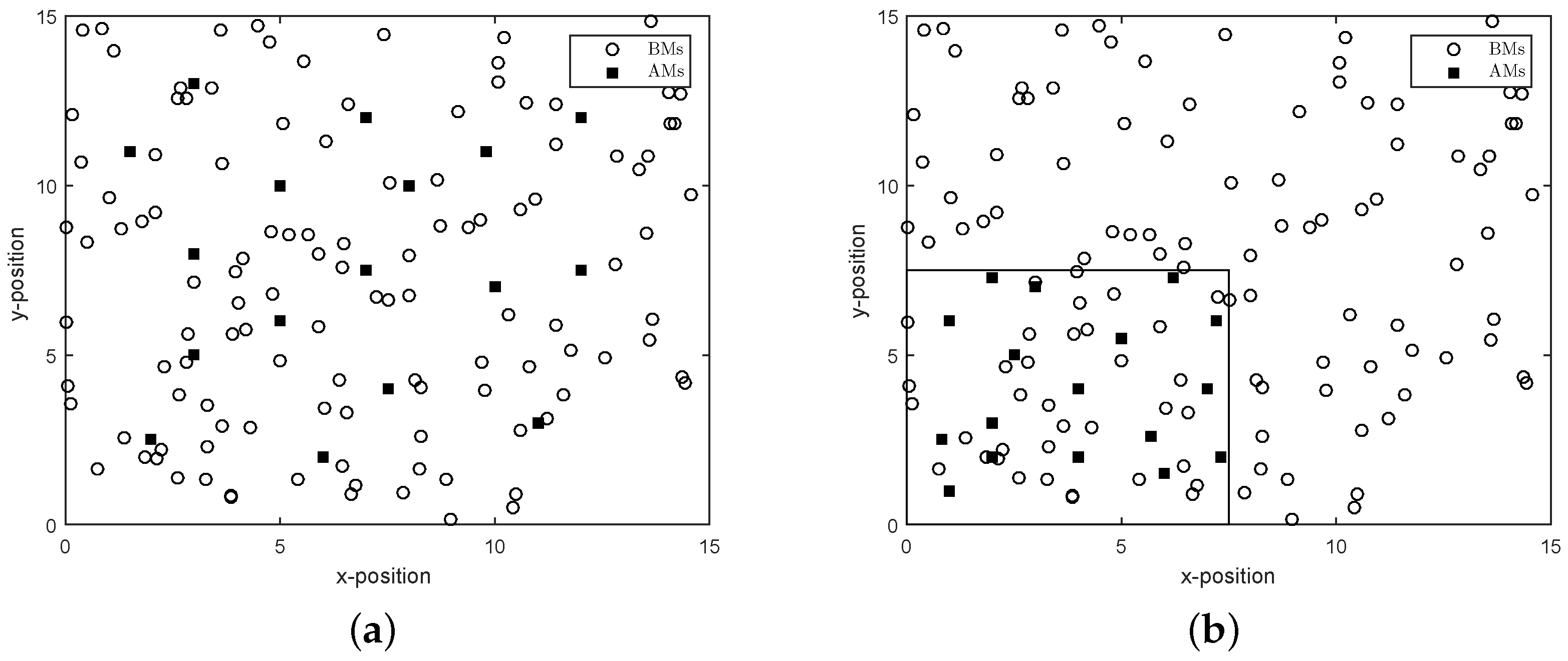
2. System Model
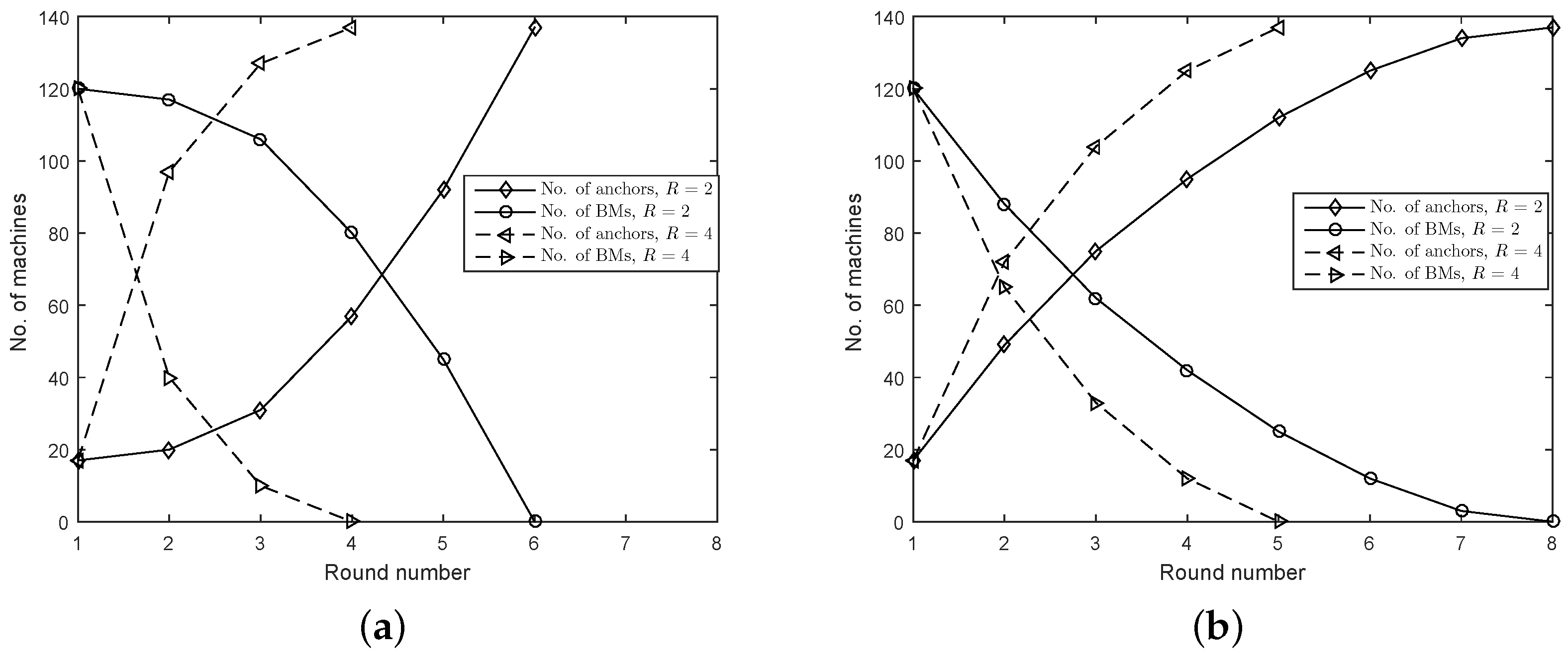
3. Greedy Successive Anchorization Process (GSAP)
3.1. Anchor Selection
3.1.1. Greedy Selection
3.1.2. Removing Collinear Anchors
3.1.3. Other Anchor Selection Methods in the Literature
3.2. Iterative Localization Algorithm
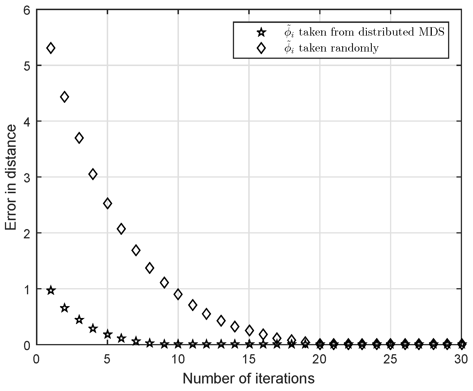
3.3. Initial Location Estimation
4. Cramér–Rao Lower Bound
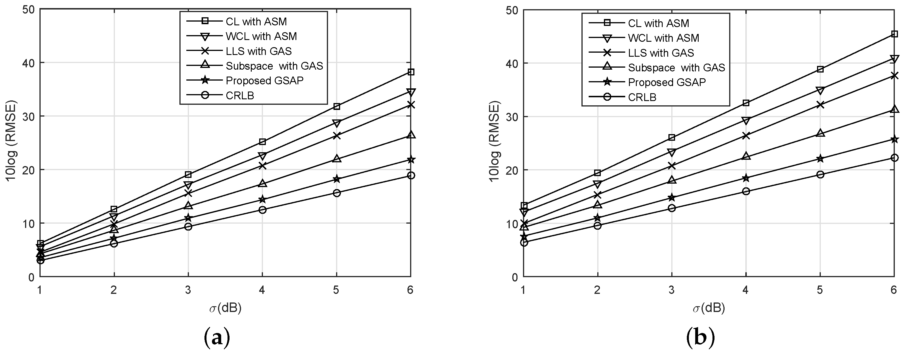
5. Numerical Results
6. Conclusions
Acknowledgments
Author Contributions
Conflicts of Interest
Abbreviations
| MTC | Machine type communication |
| AM | Anchor machine |
| BM | Blind machine |
| CRLB | Cramér–Rao lower bound |
| GPS | Global positioning system |
| CL | Centroid localization |
| WCL | Weighted centroid localization |
| RSS | Received signal strength |
| VAM | Virtual anchor machine |
| SAP | Successive anchorization process |
| GSAP | Greedy successive anchorization process |
| MDS | Multidimensional scaling |
| LLS | Linear least square |
| RMSE | Root mean square error |
| PIM | Proximity information matrix |
| FIM | Fisher information matrix |
| ASM | Anchor selection method |
| GAS | Greedy anchor selection |
References
- Verma, P.K.; Verma, R.; Prakash, A.; Agrawal, A.; Naik, K.; Tripathi, R.; Alsabaan, M.; Khalifa, T.; Abdelkader, T.; Abogharaf, A. Machine-to-Machine (M2M) communications: A survey. J. Netw. Comput. Appl. 2016, 66, 83–105. [Google Scholar] [CrossRef]
- Bourgeau, T.; Chaouchi, H.; Kirci, P. Machine-to-Machine Communications. In Next-Generation Wireless Technologies: 4G and Beyond; Chilamkurti, N., Zeadally, S., Chaouchi, H., Eds.; Springer: London, UK, 2013; pp. 221–241. [Google Scholar]
- Karim, L.; Mahmoud, Q.H.; Nasser, N.; Anpalagan, A.; Khan, N. Localization in terrestrial and underwater sensor-based M2M communication networks: Architecture, classification and challenges. Int. J. Commun. Syst. 2015. [Google Scholar] [CrossRef]
- Bal, M.; Liu, M.; Shen, W.; Ghenniwa, H. Localization in Cooperative Wireless Sensor Networks: A Review. In Proceedings of the 13rd International Conference on Computer Supported Cooperative Work in Design, Santiago, Chile, 22–24 April 2009; pp. 438–443.
- Carter, G.C. Time delay estimation for passive sonar signal processing. IEEE Trans. Acoust. Speech Signal Process. 1981, 29, 463–470. [Google Scholar] [CrossRef]
- Ehud, W. Optimal source localization and tracking from passive array measurements. IEEE Trans. Acoust. Speech Signal Process. 1982, 30, 69–76. [Google Scholar]
- Karim, L.; Nidal, N.; Mahmoud, Q.H.; Anpalagan, A.; Salti, T.E. Range-free localization approach for M2M communication system using mobile anchor nodes. J. Netw. Comput. Appl. 2015, 47, 137–146. [Google Scholar] [CrossRef]
- Neha, S.; Gazal, C.; Mehak, K. Weighted Centroid Range Free Localization Algorithm based on IoT. Int. J. Comput. Appl. 2013, 83, 27–30. [Google Scholar]
- Hu, L.; Liu, B.; Zhao, K.; Meng, X.; Wang, F. Research and Implementation of the Localization Algorithm Based on RSSI Technology. J. Netw. 2014, 9, 3135–3142. [Google Scholar] [CrossRef]
- Ibrahim, W.M.; Taha, A.E.M.; Hassanein, H.S. Scalability Issues in Localizing Things. In Proceedings of the IEEE International Conference on Local Computer Networks, Bonn, Germany, 4–7 October 2011; pp. 673–680.
- Haq, M.I.U.; Kim, D. A Novel Localization Algorithm for Internet of Things in 3D. In Proceedings of the International Conference on Information and Communication Technology Convergence, Jeju Island, Korea, 28–30 October 2015; pp. 237–241.
- Chan, F.K.W.; So, H.C. Efficient Weighted Multidimensional Scaling for Wireless Sensor Network Localization. IEEE Trans. Signal Process. 2009, 57, 4548–4553. [Google Scholar] [CrossRef]
- Kim, E.; Lee, S.; Kim, C.; Kim, K. Mobile Beacon-Based 3D-Localization with Multidimensional Scaling in Large Sensor Networks. IEEE Commun. Lett. 2010, 14, 647–649. [Google Scholar] [CrossRef]
- Savvides, A.; Garber, W.L.; Moses, R.L.; Srivastava, M.B. An analysis of error inducing parameters in multihop sensor node localization. IEEE Trans. Mob. Comput. 2005, 4, 567–577. [Google Scholar] [CrossRef]
- Rui, L.; HO, K.C. Algebraic Solution for Joint Localization and Synchronization of Multiple Sensor Nodes in the Presence of Beacon Uncertainties. IEEE Trans. Wirel. Commun. 2014, 13, 5196–5210. [Google Scholar] [CrossRef]
- Chiu, W.Y.; Chen, B.S.; Yang, C.Y. Robust Relative Location Estimation in Wireless Sensor Networks with Inexact Position Problems. IEEE Trans. Mob. Comput. 2012, 11, 935–946. [Google Scholar] [CrossRef]
- Borg, I.; Groenen, P.J.F. Modern Multidimensional Scaling: Theory and Applications, 2nd ed.; Springer: New York, NY, USA, 2005. [Google Scholar]
- Lohrasbipeydeh, H.; Gulliver, T.A.; Amindavar, H. Blind received signal strength difference based source localization with system parameter errors. IEEE Trans. Signal Process. 2014, 62, 4516–4531. [Google Scholar] [CrossRef]
- Moore, D.; Leonard, J.; Rus, D.; Teller, S. Robust Distributed Network Localization with Noisy Range Measurements. In Proceedings of the 2nd International Conference on Embedded Networked Sensor Systems, Baltimore, MD, USA, 3–5 November 2004; pp. 50–61.
- Hendrickson, B. Conditions for unique graph realizations. SIAM J. Comput. 1992, 21, 65–84. [Google Scholar] [CrossRef]
- Ermel, E.; Fladenmuller, A.; Pujolle, G.; Cotton, A. On Selecting Nodes to Improve Estimated Positions. In Proceedings of the IFIP TC6/WG6.8 Conference on Mobile and Wireless Communication Networks, Paris, France, 25–27 October 2004; pp. 449–460.
- Ji, Y.; Biaz, S.; Wu, S.; Qi, B. Optimal sniffers deployment on wireless indoor localization. In Proceedings of the IEEE International Conference Computer Communications and Networks, Honolulu, HI, USA, 13–16 August 2007; pp. 251–256.
- Beck, A. Introduction to Nonlinear Optimization: Theory, Algorithms, and Applications with MATLAB; Society for Industrial and Applied Mathematics: Philadelphia, PA, USA, 2014. [Google Scholar]
- Yu, T.M.; Jian, X.D.; Liang, S.J.; Yan, S. Application of the Newton-Raphson Method in a Voice Localization System. Appl. Mech. Mater. 2014, 513, 4435–4438. [Google Scholar]
- Chepuri, S.P.; Leus, G. Sparsity-Promoting Sensor Selection for Non-Linear Measurement Models. IEEE Trans. Signal Process. 2015, 63, 684–698. [Google Scholar] [CrossRef]
- Rudich, S.; Wigderson, A. Computational Complexity Theory; American Mathematical Society: Providence, RI, USA, 2004. [Google Scholar]
- Hamdi, M.; Boudriga, N.; Obaidat, M.S. Bandwidth-Effective Design of a Satellite-Based Hybrid Wireless Sensor Network for Mobile Target Detection and Tracking. IEEE Syst. J. 2008, 2, 74–82. [Google Scholar] [CrossRef]
- Kay, S.M. Fundamentals of Statistical Signal Processing: Estimation Theory, 1st ed.; Prentice Hall PTR: Upper Saddle River, NJ, USA, 1993. [Google Scholar]
- So, H.C.; Lin, L. Linear Least Squares Approach for Accurate Received Signal Strength Based Source Localization. IEEE Trans. Signal Process. 2011, 59, 4035–4040. [Google Scholar] [CrossRef]
- Kruskal, J.B. On the shortest spanning subtree of a graph and the traveling salesman problem. Proc. Am. Math. Soc. 1956, 7, 48–50. [Google Scholar] [CrossRef]
- Wei, H.W.; Wan, Q.; Chen, Z.X.; Ye, S.F. A Novel Weighted Multidimensional Scaling Analysis for Time-of-Arrival-Based Mobile Location. IEEE Trans. Signal Process. 2008, 56, 3018–3022. [Google Scholar] [CrossRef]
- Trees, H.L.V. Detection, Estimation, and Modulation Theory; John Wiley & Sons: New York, NY, USA, 2004. [Google Scholar]
- Shen, Y.; Win, M.Z. Performance of Localization and Orientation Using Wideband Antenna Arrays. In Proceedings of the IEEE International Conference on Ultra-Wideband, Marina Mandarin, Singapore, 24–26 September 2007; pp. 288–293.
- Patwari, N.; Hero, A.O.; Perkins, M.; Correal, N.S.; O’Dea, R.J. Relative location estimation in wireless sensor networks. IEEE Trans. Signal Process. 2003, 51, 2137–2148. [Google Scholar] [CrossRef]
- Haq, M.I.U.; Kim, D. Improved Localization by Time of Arrival for Internet of Things in 3D. In Proceedings of the International Conference on Applied Electromagnetics and Communications, Dubrovnik, Croatia, 19–21 September 2016.

| Symbol | Description |
|---|---|
| N | Total number of AMs and BMs |
| n | Total number of BMs at the start of localization process |
| m | Total number of AMs |
| Total number of VAMs | |
| Total number of BMs | |
| Total number of anchors (i.e., AMs plus VAMs) | |
| Actual position vector of machines | |
| Actual position vector of BMs | |
| Actual position vector of VAMs | |
| Estimated position of VAMs | |
| Set of AMs | |
| Set of VAMs | |
| Set of BMs | |
| Set of selected anchors who will participate in localization | |
| Expected position error (scalar) | |
| Expected error in measurement (scalar) | |
| P | Transmitted power (scalar) |
| ς | Power loss in dB (scalar) |
| η | RSS noise (scalar) |
| β | Distance-power gradient (scalar) |
| d | Actual distance (scalar) |
| Observed range (scalar) | |
| ζ | Weight for anchors based on and which is used in anchor selection (scalar) |
| Observed path loss in dB (vector) | |
| Π | Jacobian matrix |
| Initial position vector for BMs | |
| Wieghting matrix used in weighted least square formulation | |
| Final estimated position vector for BMs | |
| Proximity information matrix | |
| Ω | Double centered matrix |
| ϱ | Actual position vector of all BMs |
| Covariance matrix for error in which we assume a white Gaussian process | |
| Bias of an estimator (vector) | |
| ℧ | Covariance matrix of an estimator |
| Ψ | Mean square error matrix |
| Expectation operator | |
| Γ | Fisher information matrix |
| Stress function used in multidimensional scaling | |
| Log-likelihood function | |
| Probability density function | |
| Inverse of a matrix | |
| Transpose of a vector or matrix | |
| Trace of a matrix |
© 2016 by the authors; licensee MDPI, Basel, Switzerland. This article is an open access article distributed under the terms and conditions of the Creative Commons Attribution (CC-BY) license (http://creativecommons.org/licenses/by/4.0/).
Share and Cite
Imtiaz Ul Haq, M.; Kim, D. Greedy Successive Anchorization for Localizing Machine Type Communication Devices. Sensors 2016, 16, 2115. https://doi.org/10.3390/s16122115
Imtiaz Ul Haq M, Kim D. Greedy Successive Anchorization for Localizing Machine Type Communication Devices. Sensors. 2016; 16(12):2115. https://doi.org/10.3390/s16122115
Chicago/Turabian StyleImtiaz Ul Haq, Mian, and Dongwoo Kim. 2016. "Greedy Successive Anchorization for Localizing Machine Type Communication Devices" Sensors 16, no. 12: 2115. https://doi.org/10.3390/s16122115
APA StyleImtiaz Ul Haq, M., & Kim, D. (2016). Greedy Successive Anchorization for Localizing Machine Type Communication Devices. Sensors, 16(12), 2115. https://doi.org/10.3390/s16122115