
LPI Radar Waveform Recognition Based on Time-Frequency Distribution


Abstract
:1. Introduction
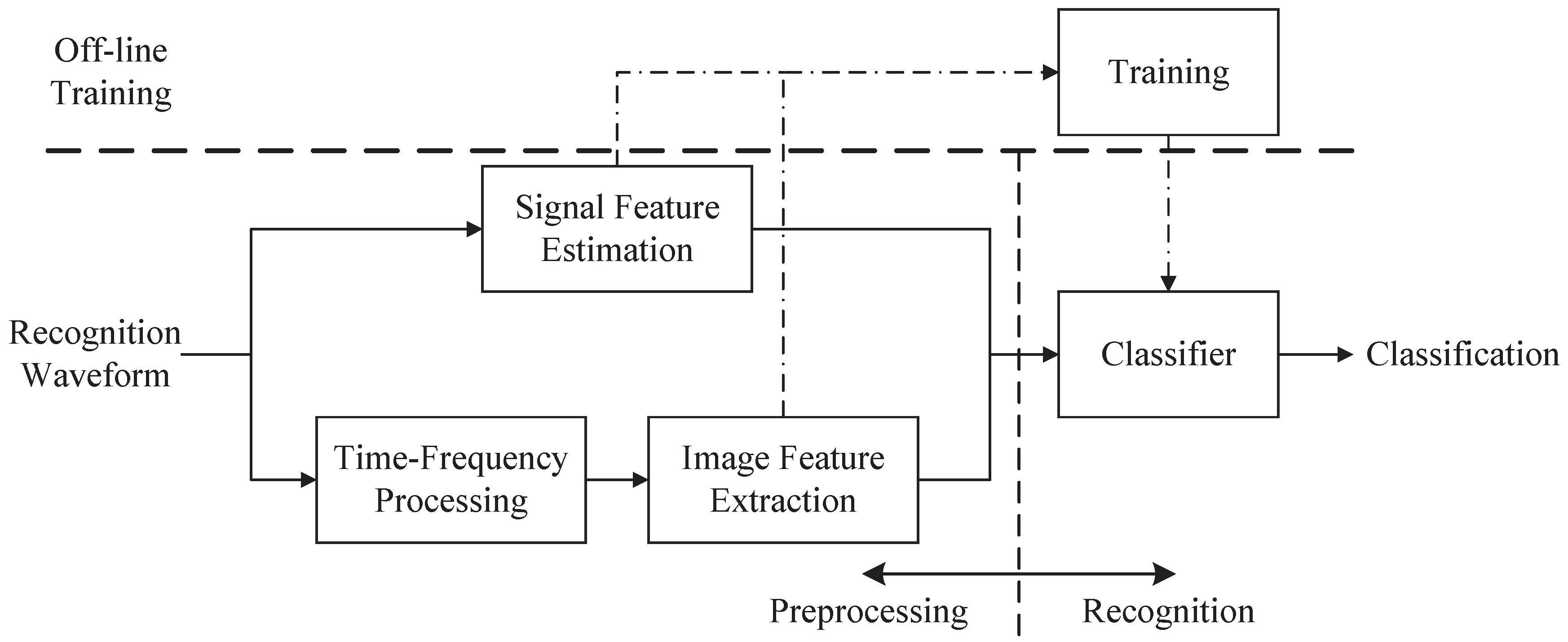
2. System Overview
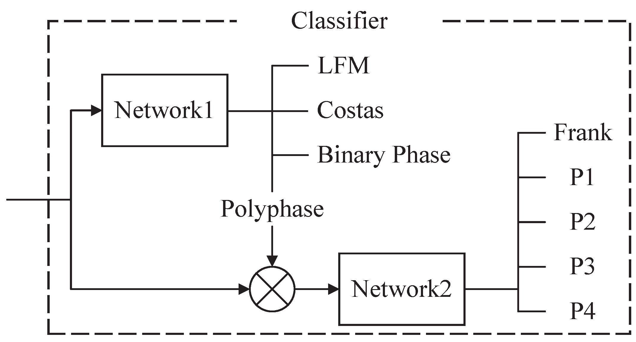
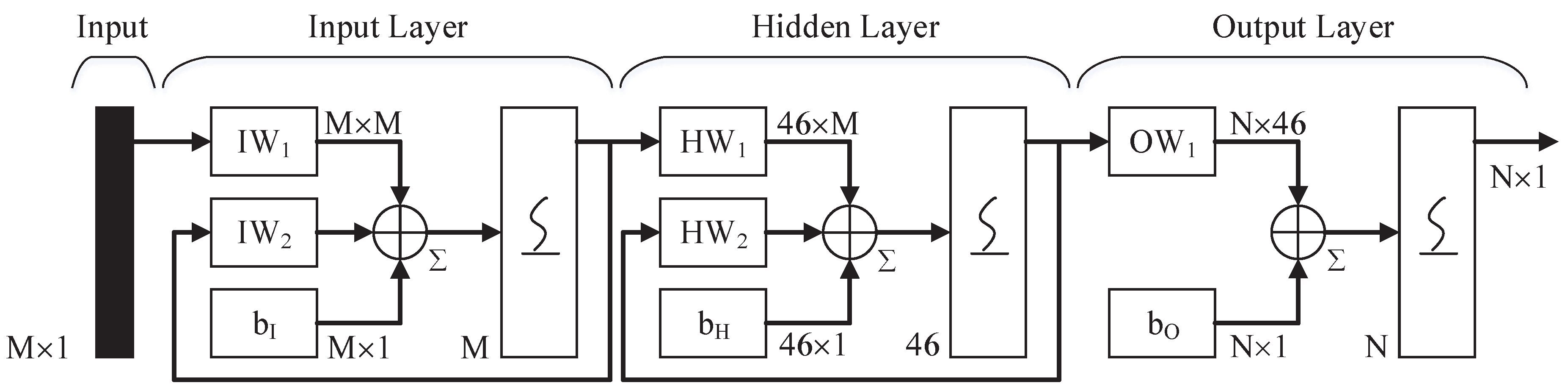
3. Waveform Classifier
4. Features Extraction
4.1. Signal Features
4.1.1. Based on Second Order Statistics
4.1.2. Based on Power Spectral Density (PSD)
4.1.3. Based on Instantaneous Properties
- calculate ;
- compute from ;
- set ;
- calculate ;
- calculate the normalized centered instantaneous frequency , i.e.;
- the absolute value of the normalized centered instantaneous frequency is given by;
- *
- corrects the radian phase angles in by adding multiples of when absolute jumps between consecutive element of is greater than or equal to the jump tolerance of π radians.
- **
- There are some spikes in the instantaneous frequency estimation in the vicinity of phase discontinuity of some waveforms. In order to smooth the and to remove the spikes, a median-filter with window size 5 is used.
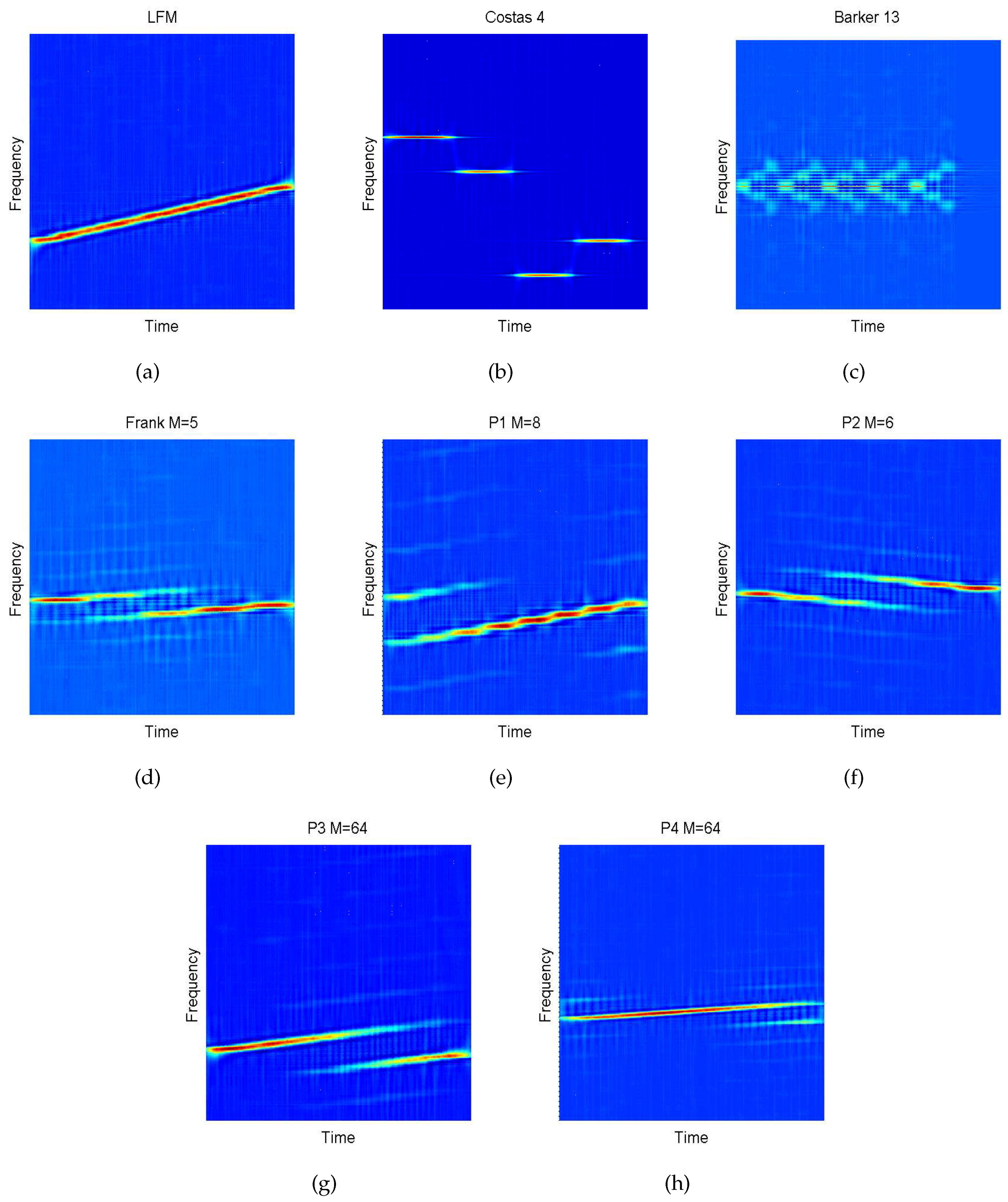
4.2. Choi–Williams Distribution (CWD)
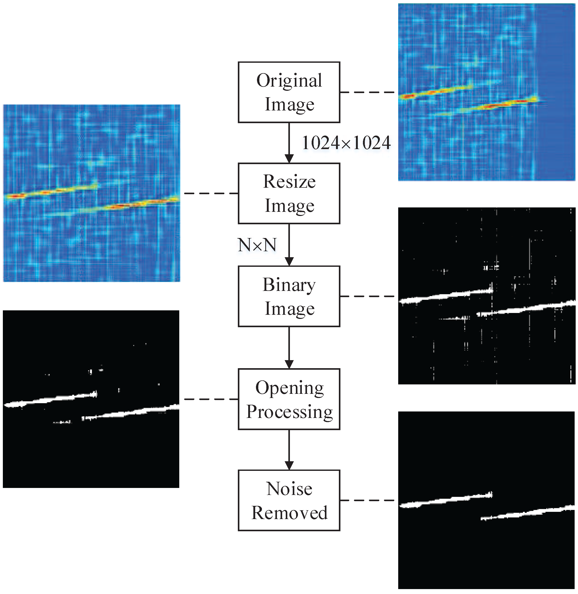
4.3. Image Preprocessing
- transform the resized image to gray image between , i.e.;
- estimate the initial threshold T. It can be obtained from the average of the minimum and maximum from the image ;
- divide the image into two pixel groups and after the comparison with the threshold T. includes all pixels in the image that the values , and includes all pixels in the image that the values ;
- calculate the average value and of two pixel groups and , respectively;
- update the threshold value;
- repeat (b–e), and calculate , i.e.;
- until the is smaller than a predefined convergence value, 0.001 is used in the paper;
- calculate ;
- output the final binary image .
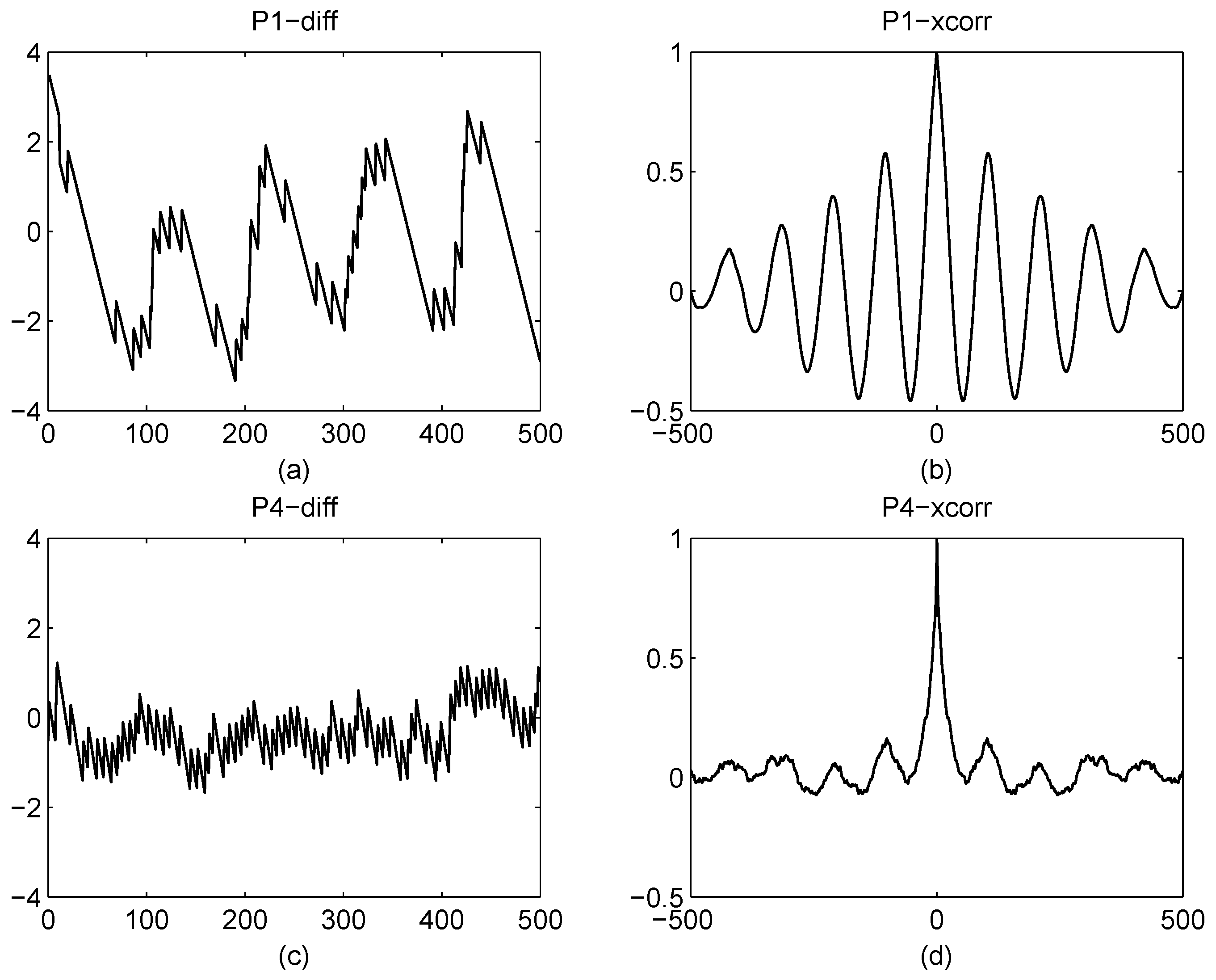
4.4. Image Features
- for each object, ;
- decide the k and mask the other objects away from the binary image;
- calculate the principal components of the binary image;
- rotate∗ the image until the principal component of the object is parallel to the vertical axis, recorded as ;
- calculate the row sum, i.e., , ;
- normalize , i.e., ;
- calculate the standard deviation of , i.e.,where N is the number of samples.
- output the rotation degree of the maximum of objects ;
- output the average of the , i.e.;
- *
- nearest neighbor interpolation is used in rotation processing.
- calculate the average of ;
- calculate as follows , ;
- a consecutive sequence of 0’s or 1’s is called a unit, and R is the number of units. Let and denote the statistics number of and , respectively, i.e., ;
- calculate the mean of units, i.e.;
- calculate the variance of units, i.e.;
- calculate the value of test statistic Y, i.e.;
- output the probability feature, i.e.;
- *
- where is the standard normal cumulative distribution function. The value of is between 0 and 1.
- **
- note that is no longer a probability. It is a measure of the similarity with Gaussian distribution. The standard deviation value is too small for machine precision. Therefore, it is replaced by variance in (f).
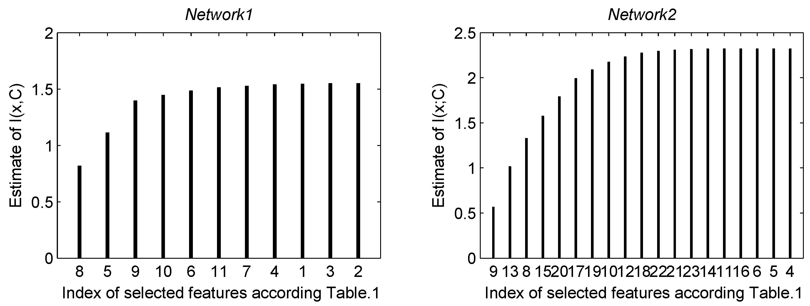
5. Features Selection
6. Simulation and Discussion
6.1. Create Simulation Signals
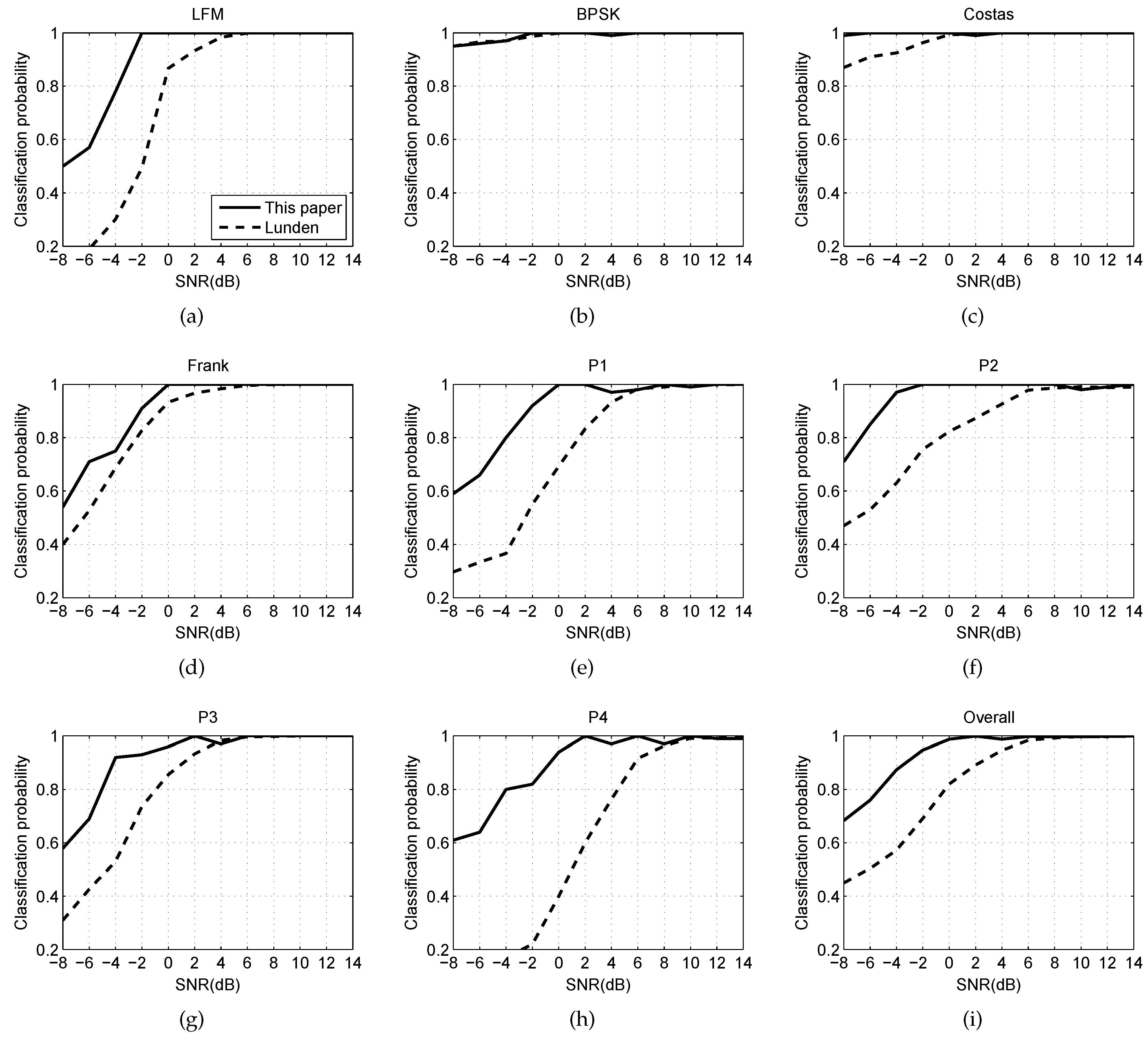
6.2. Experiment With SNR
6.3. Experiment with Robustness
6.4. Experiment with Computation
7. Conclusions
Acknowledgments
Author Contributions
Conflicts of Interest
Abbreviations
| LPI | Low Probability of Intercept |
| LFM | Linear Frequency Modulation |
| FM | Frequency Modulation |
| ENN | Elman Neural Network |
| BPSK | Binary Phase Shift Keying |
| FMCW | Frequency Modulated Continuous Wave |
| CWD | Choi–Williams Time-Frequency Distribution |
| PSK | Phase Shift Keying |
| FSK | Frequency Shift Keying |
| PCA | Principal Component Analysis |
| RSR | Ratio of Successful Recognition |
| SNR | Signal-to-Noise Ratio |
| EW | Electronic Warfare |
| STFT | Short-Time Fourier Transform |
| WVD | Wigner–Ville Distribution |
| PWD | Pseudo–Wigner Distribution |
| RD | Rihaczek Distribution |
| HT | Hough Transform |
| AWGN | Additive White Gaussian Noise |
| PSD | Power Spectral Density |
References
- Fuller, K. To see and not be seen (radar). IEE Proc. F-Radar Signal Proc. 1990, 137, 1–9. [Google Scholar] [CrossRef]
- Nandi, A.K.; Azzouz, E.E. Algorithms for automatic modulation recognition of communication signals. IEEE Trans. Commun. 1998, 46, 431–436. [Google Scholar] [CrossRef]
- Nandi, A.; Azzouz, E. Automatic analogue modulation recognition. Signal Proc. 1995, 46, 211–222. [Google Scholar] [CrossRef]
- Cohen, L. Time-frequency distributions: A review. Proc. IEEE 1989, 77, 941–981. [Google Scholar] [CrossRef]
- Barbarossa, S. Analysis of multicomponent LFM signals by a combined Wigner-Hough transform. IEEE Trans. Signal Proc. 1995, 43, 1511–1515. [Google Scholar] [CrossRef]
- Barbarossa, S.; Lemoine, O. Analysis of nonlinear FM signals by pattern recognition of their time-frequency representation. IEEE Signal Proc. Lett. 1996, 3, 112–115. [Google Scholar] [CrossRef]
- López-Risueño, G.; Grajal, J.; Sanz-Osorio, Á. Digital channelized receiver based on time-frequency analysis for signal interception. IEEE Trans. Aerosp. Electron. Syst. 2005, 41, 879–898. [Google Scholar] [CrossRef]
- Lopez-Risueno, G.; Grajal, J.; Yeste-Ojeda, O. Atomic decomposition-based radar complex signal interception. IEE Proc. Radar Sonar Navig. 2003, 150, 323–331. [Google Scholar] [CrossRef]
- Zilberman, E.R.; Pace, P.E. Autonomous time-frequency morphological feature extraction algorithm for LPI radar modulation classification. In Proceedings of the 2006 IEEE International Conference on Image Processing, Atlanta, GA, USA, 8–11 October 2006; pp. 2321–2324.
- Pace, P.E. Detecting and Classifying Low Probability of Intercept Radar, 2nd ed.; Artech House: Norwood, MA, USA, 2009. [Google Scholar]
- Lundén, J.; Koivunen, V. Automatic radar waveform recognition. IEEE J. Sel. Top. Signal Proc. 2007, 1, 124–136. [Google Scholar] [CrossRef]
- Zeng, D.; Zeng, X.; Cheng, H.; Tang, B. Automatic modulation classification of radar signals using the Rihaczek distribution and Hough transform. IET Radar Sonar Navig. 2012, 6, 322–331. [Google Scholar] [CrossRef]
- Ma, J.; Huang, G.; Zuo, W.; Wu, X.; Gao, J. Robust radar waveform recognition algorithm based on random projections and sparse classification. IET Radar Sonar Navig. 2013, 8, 290–296. [Google Scholar] [CrossRef]
- Chen, B.; Shu, H.; Zhang, H.; Chen, G.; Toumoulin, C.; Dillenseger, J.L.; Luo, L.M. Quaternion Zernike moments and their invariants for color image analysis and object recognition. Signal Proc. 2012, 92, 308–318. [Google Scholar] [CrossRef]
- Xu, B.; Sun, L.; Xu, L.; Xu, G. Improvement of the Hilbert method via ESPRIT for detecting rotor fault in induction motors at low slip. IEEE Trans. Energy Convers. 2013, 28, 225–233. [Google Scholar] [CrossRef]
- Johnson, A.E.; Ghassemi, M.M.; Nemati, S.; Niehaus, K.E.; Clifton, D.; Clifford, G.D. Machine learning and decision support in critical care. Proc. IEEE 2016, 104, 444–466. [Google Scholar] [CrossRef]
- Bengio, Y.; Courville, A.; Vincent, P. Representation learning: A review and new perspectives. IEEE Trans. Pattern Anal. Mach. Intell. 2013, 35, 1798–1828. [Google Scholar] [CrossRef] [PubMed]
- Lin, W.M.; Hong, C.M.; Chen, C.H. Neural-network-based MPPT control of a stand-alone hybrid power generation system. IEEE Trans. Power Electron. 2011, 26, 3571–3581. [Google Scholar] [CrossRef]
- Lin, C.M.; Boldbaatar, E.A. Autolanding control using recurrent wavelet Elman neural network. IEEE Trans. Syst. Man Cybern. Syst. 2015, 45, 1281–1291. [Google Scholar] [CrossRef]
- Sheela, K.G.; Deepa, S. Review on methods to fix number of hidden neurons in neural networks. Math. Probl. Eng. 2013, 2013. [Google Scholar] [CrossRef]
- Zhu, Z.; Aslam, M.W.; Nandi, A.K. Genetic algorithm optimized distribution sampling test for M-QAM modulation classification. Signal Proc. 2014, 94, 264–277. [Google Scholar] [CrossRef]
- Ozen, A.; Ozturk, C. A novel modulation recognition technique based on artificial bee colony algorithm in the presence of multipath fading channels. In Proceedings of the 36th IEEE International Conference on Elecommunications and Signal Processing (TSP), Rome, Italy, 2–4 July 2013; pp. 239–243.
- Venäläinen, J.; Terho, L.; Koivunen, V. Modulation classification in fading multipath channel. In Proceedings of the 2002 Conference Record of the 36th Asilomar Conference on Signals, Systems and Computers, Pacific Grove, CA, USA, 3–6 November 2002; pp. 1890–1894.
- Stoica, P.; Moses, R.L. Spectral Analysis of Signals; Prentice Hall: Upper Saddle River, NJ, USA, 2005. [Google Scholar]
- Wong, M.D.; Nandi, A.K. Automatic digital modulation recognition using artificial neural network and genetic algorithm. Signal Proc. 2004, 84, 351–365. [Google Scholar] [CrossRef]
- Feng, Z.; Liang, M.; Chu, F. Recent advances in time–frequency analysis methods for machinery fault diagnosis: A review with application examples. Mech. Syst. Signal Proc. 2013, 38, 165–205. [Google Scholar] [CrossRef]
- Gonzalez, R.C. Digital Image Processing; Pearson Education: Delhi, India, 2009. [Google Scholar]
- Chen, Z.; Sun, S.K. A Zernike moment phase-based descriptor for local image representation and matching. IEEE Trans. Image Proc. 2010, 19, 205–219. [Google Scholar] [CrossRef] [PubMed]
- Tan, C.W.; Kumar, A. Accurate iris recognition at a distance using stabilized iris encoding and Zernike moments phase features. IEEE Trans. Image Proc. 2014, 23, 3962–3974. [Google Scholar] [CrossRef] [PubMed]
- Honarvar, B.; Paramesran, R.; Lim, C.L. Image reconstruction from a complete set of geometric and complex moments. Signal Proc. 2014, 98, 224–232. [Google Scholar] [CrossRef]
- Kwak, N.; Choi, C.H. Input feature selection by mutual information based on Parzen window. IEEE Trans. Pattern Anal. Mach. Intell. 2002, 24, 1667–1671. [Google Scholar] [CrossRef]
- Van Hulle, M.M. Edgeworth approximation of multivariate differential entropy. Neural Comput. 2005, 17, 1903–1910. [Google Scholar] [CrossRef] [PubMed]


| Index | Features | Network1 | Network2 |
|---|---|---|---|
| 1 | Moment | ✔ | |
| 2 | Moment | ✔ | |
| 3 | Cumulant | ✔ | |
| 4 | PSD maximum | ✔ | ✔ |
| 5 | PSD maximum | ✔ | ✔ |
| 6 | Std. of instantaneous phase | ✔ | ✔ |
| 7 | Std. of instantaneous freq. | ✔ | |
| 8 | Num. of objects (10%) | ✔ | ✔ |
| 9 | Num. of objects (50%) | ✔ | ✔ |
| 10 | CWD time peak location | ✔ | ✔ |
| 11 | Std. of object width | ✔ | ✔ |
| 12 | Maximum of PCA degree | ✔ | |
| 13 | Std. of | ✔ | |
| 14 | Statistics test | ✔ | |
| 15 | Autocorr. of r | ✔ | |
| 16 | FFT of corr. | ✔ | |
| 17 | Pseudo–Zernike moment | ✔ | |
| 18 | Pseudo–Zernike moment | ✔ | |
| 19 | Pseudo–Zernike moment | ✔ | |
| 20 | Pseudo–Zernike moment | ✔ | |
| 21 | Pseudo–Zernike moment | ✔ | |
| 22 | Pseudo–Zernike moment | ✔ | |
| 23 | Pseudo–Zernike moment | ✔ |
| Radar Waveforms | Parameter | Ranges |
|---|---|---|
| - | Sampling rate | 1 |
| LFM | Initial frequency | |
| Bandwidth | ||
| Number of samples | ||
| BPSK | Carrier frequency | |
| Barker codes | ||
| Number of code periods | ||
| Cycles per phase code | ||
| Costas codes | Number change | |
| Fundamental frequency | ||
| N | ||
| Frank & P1 code | ||
| M | ||
| P2 code | ||
| M | ||
| P3 & P4 code | ||
| M |
| LFM | BPSK | Costas | Frank | P1 | P2 | P3 | P4 | |
|---|---|---|---|---|---|---|---|---|
| LFM | 100 | 0 | 0 | 0 | 0 | 0 | 0 | 18 |
| BPSK | 0 | 100 | 0 | 0 | 0 | 0 | 0 | 0 |
| Costas | 0 | 0 | 100 | 1 | 0 | 0 | 0 | 0 |
| Frank | 0 | 0 | 0 | 91 | 3 | 0 | 4 | 0 |
| P1 | 0 | 0 | 0 | 0 | 92 | 0 | 0 | 0 |
| P2 | 0 | 0 | 0 | 0 | 0 | 100 | 0 | 0 |
| P3 | 0 | 0 | 0 | 8 | 0 | 0 | 93 | 0 |
| P4 | 0 | 0 | 0 | 0 | 5 | 0 | 3 | 82 |
| Item | Model/Version |
|---|---|
| CPU | E5-1620V2 (Intel) |
| Memory | 16 GB (DDR3@1600 MHz) |
| GPU | NVS315 (Quadro) |
| MATLAB | R2012a |
| LFM | BPSK | Costas | Frank | |
| −8 dB | 55.604/86.324 | 51.332/82.374 | 54.875/84.279 | 56.336/87.022 |
| −2 dB | 54.979/86.111 | 51.195/81.560 | 54.009/84.183 | 56.294/86.654 |
| 10 dB | 54.783/85.899 | 50.867/81.055 | 53.336/83.807 | 55.793/86.131 |
| P1 | P2 | P3 | P4 | |
| −8 dB | 58.628/88.282 | 56.754/88.360 | 58.830/87.798 | 54.895/85.999 |
| −2 dB | 58.422/87.923 | 55.801/88.180 | 58.107/87.353 | 54.428/85.187 |
| 10 dB | 57.679/87.005 | 55.368/87.448 | 57.505/86.901 | 53.900/84.533 |
© 2016 by the authors; licensee MDPI, Basel, Switzerland. This article is an open access article distributed under the terms and conditions of the Creative Commons Attribution (CC-BY) license (http://creativecommons.org/licenses/by/4.0/).
Share and Cite
Zhang, M.; Liu, L.; Diao, M. LPI Radar Waveform Recognition Based on Time-Frequency Distribution. Sensors 2016, 16, 1682. https://doi.org/10.3390/s16101682
Zhang M, Liu L, Diao M. LPI Radar Waveform Recognition Based on Time-Frequency Distribution. Sensors. 2016; 16(10):1682. https://doi.org/10.3390/s16101682
Chicago/Turabian StyleZhang, Ming, Lutao Liu, and Ming Diao. 2016. "LPI Radar Waveform Recognition Based on Time-Frequency Distribution" Sensors 16, no. 10: 1682. https://doi.org/10.3390/s16101682
APA StyleZhang, M., Liu, L., & Diao, M. (2016). LPI Radar Waveform Recognition Based on Time-Frequency Distribution. Sensors, 16(10), 1682. https://doi.org/10.3390/s16101682