
Application of a Terrestrial LIDAR System for Elevation Mapping in Terra Nova Bay, Antarctica


Abstract
:1. Introduction
2. Experimental Section
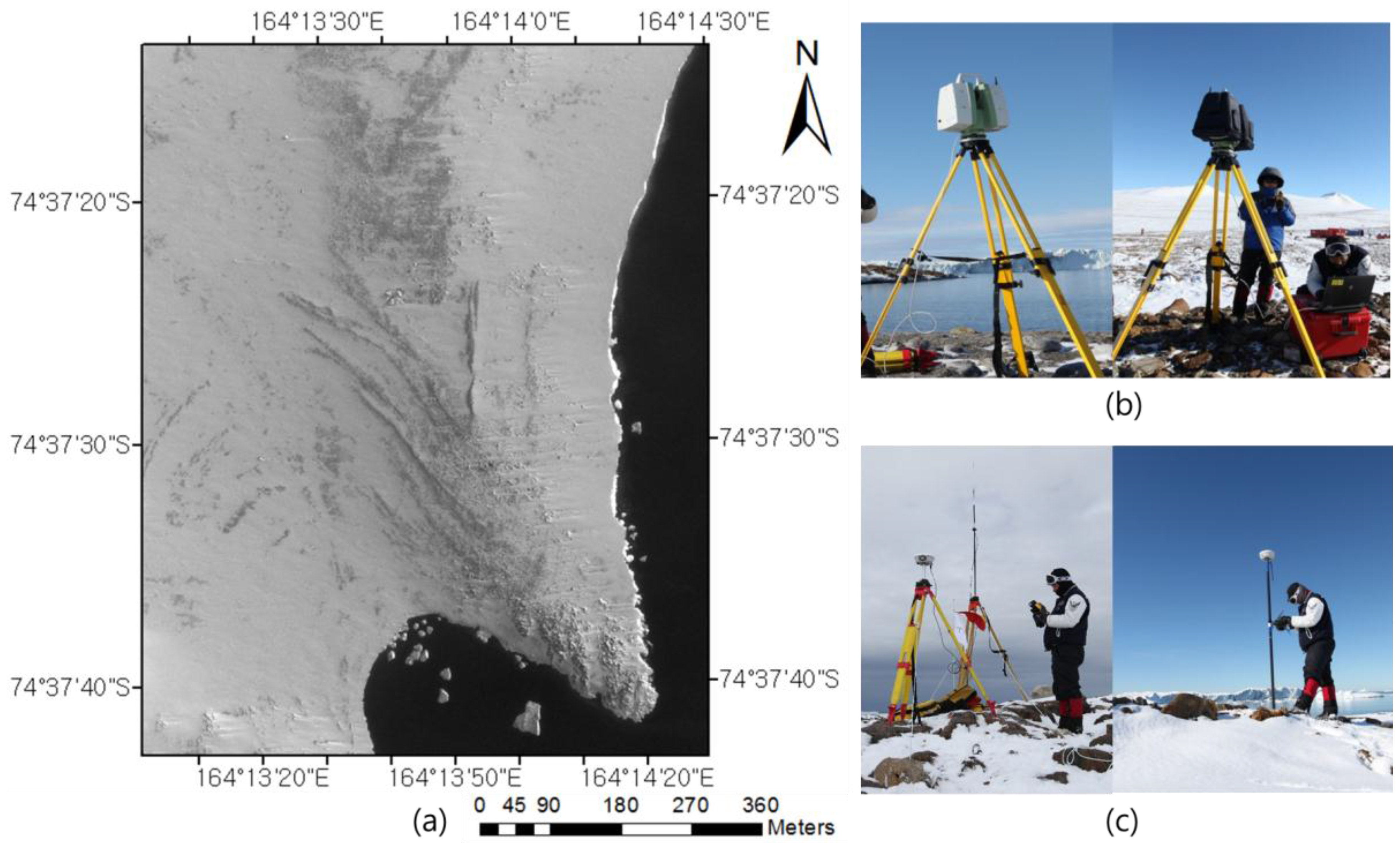
2.1. Study Area
2.2. Overview of Methodology
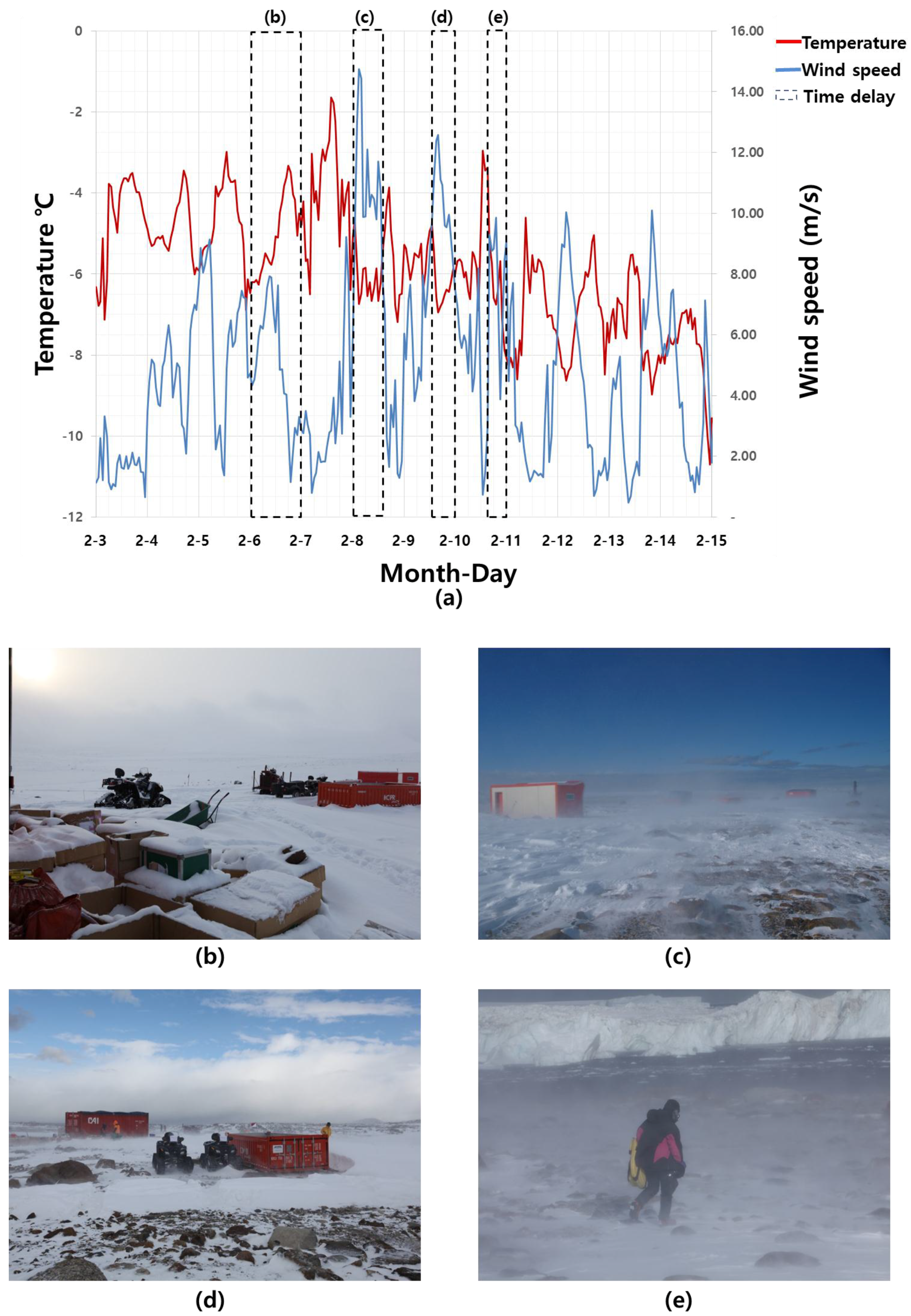
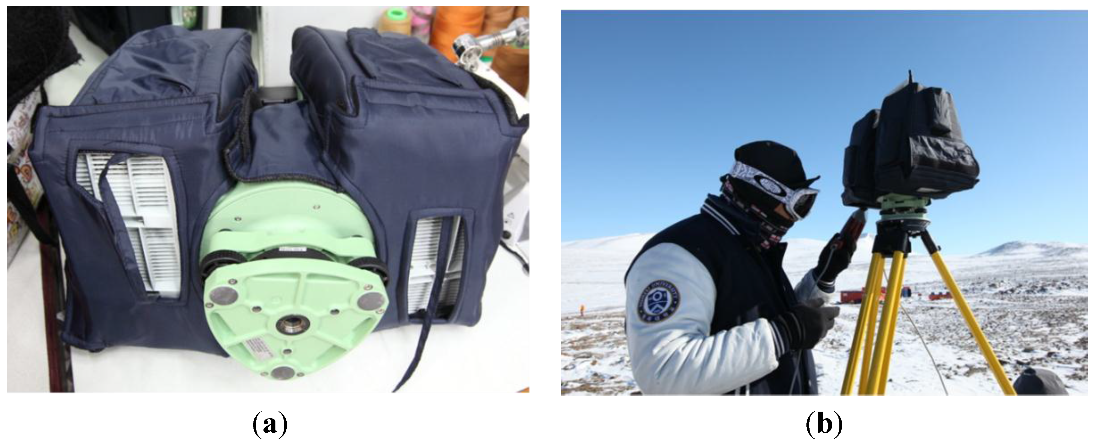
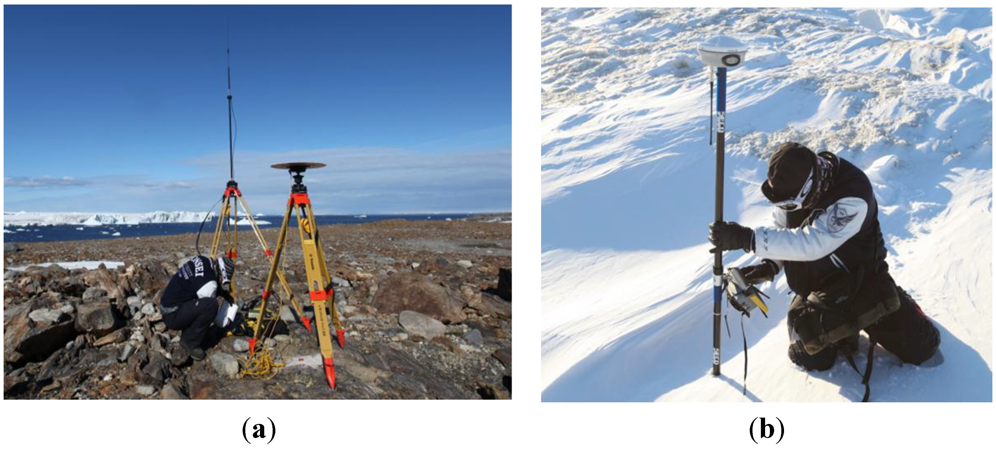
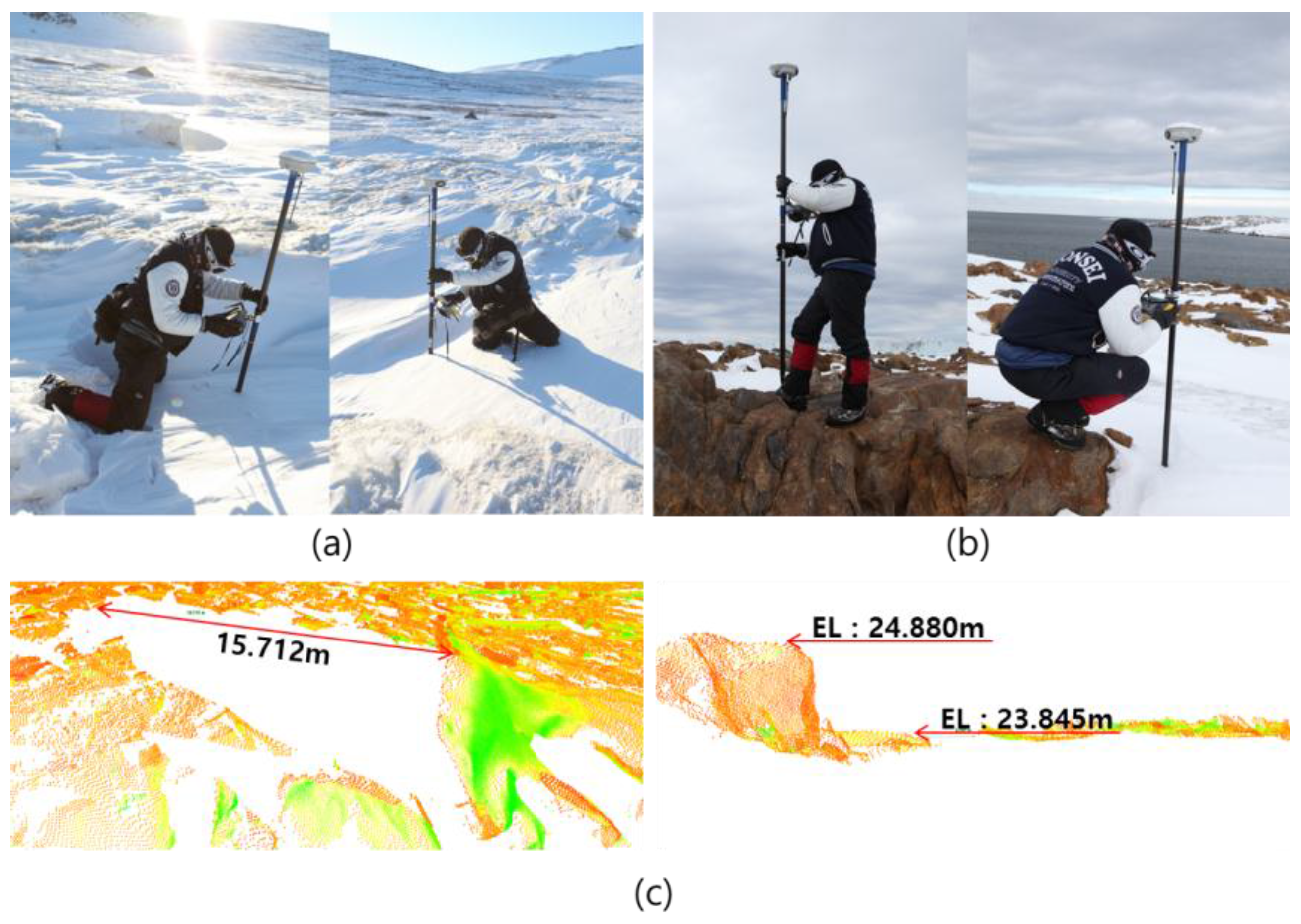
2.3. Operational Phase

| ScanStation C10 | Specification | |
|---|---|---|
| Type | Pulsed | |
| Wavelength | 532 nm | |
| Range | 300 m at 90% albedo, 134 m at 18% albedo (minimum range 0.1 m) | |
| Scan rate | Up to 50,000 points/s (maximum instantaneous rate) | |
| Accuracy of single measurement * | Position | 6 mm |
| Distance | 4 mm | |
| Angle | 60 µrad | |
| Field of view | Horizontal | 360° (maximum) |
| Vertical | 270° (maximum) | |
| Weight | 13 kg | |
| Size (depth, width, height) | 238, 358, 395 mm | |
| Operating temperature | 0 °C to +40 °C | |
| Storage temperature | −25 °C to +65 °C | |
| Camera | Auto-adjusting, integrated high-resolution digital camera with zoom video | |
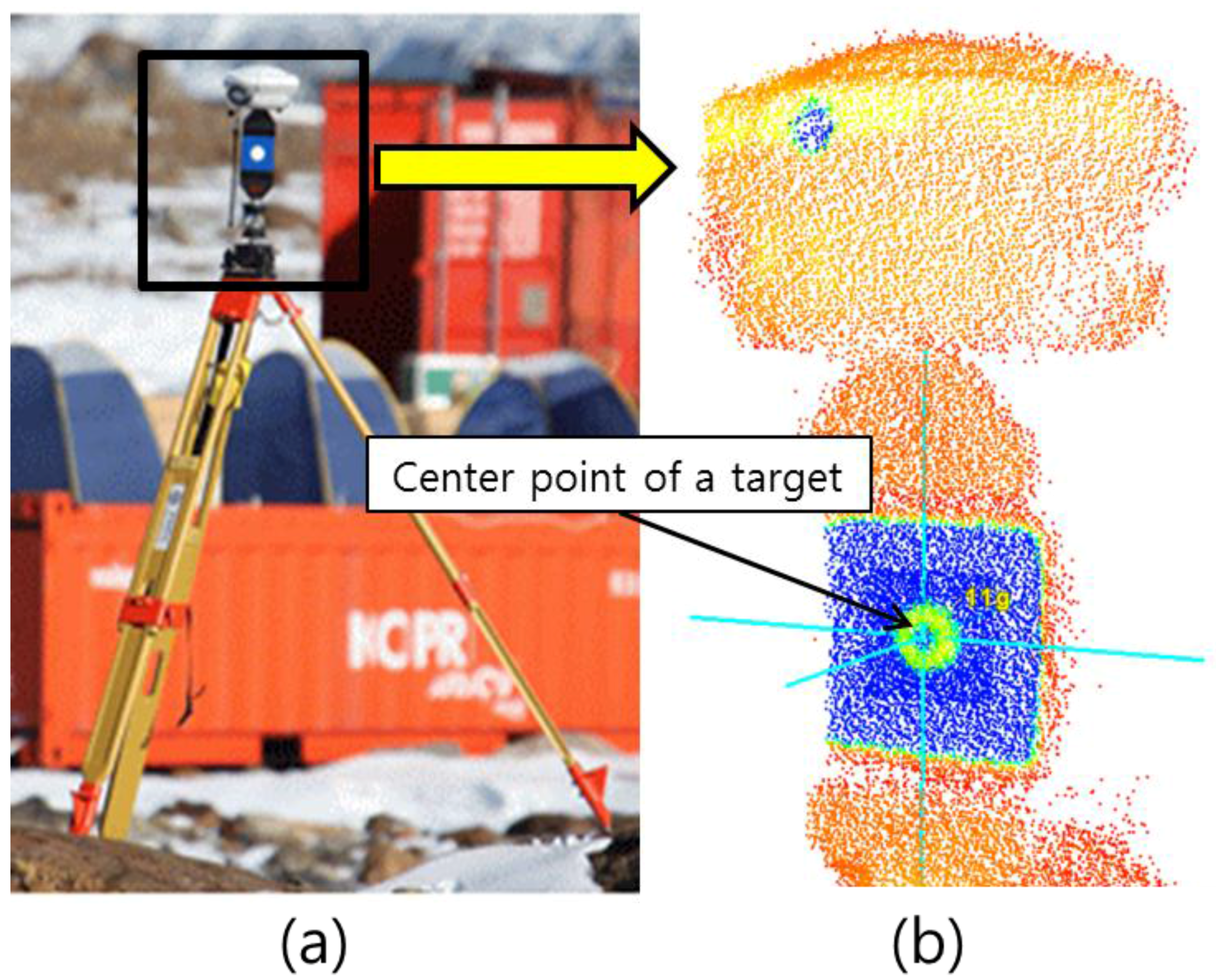
2.4. Co-Registration and Georeferencing Phases
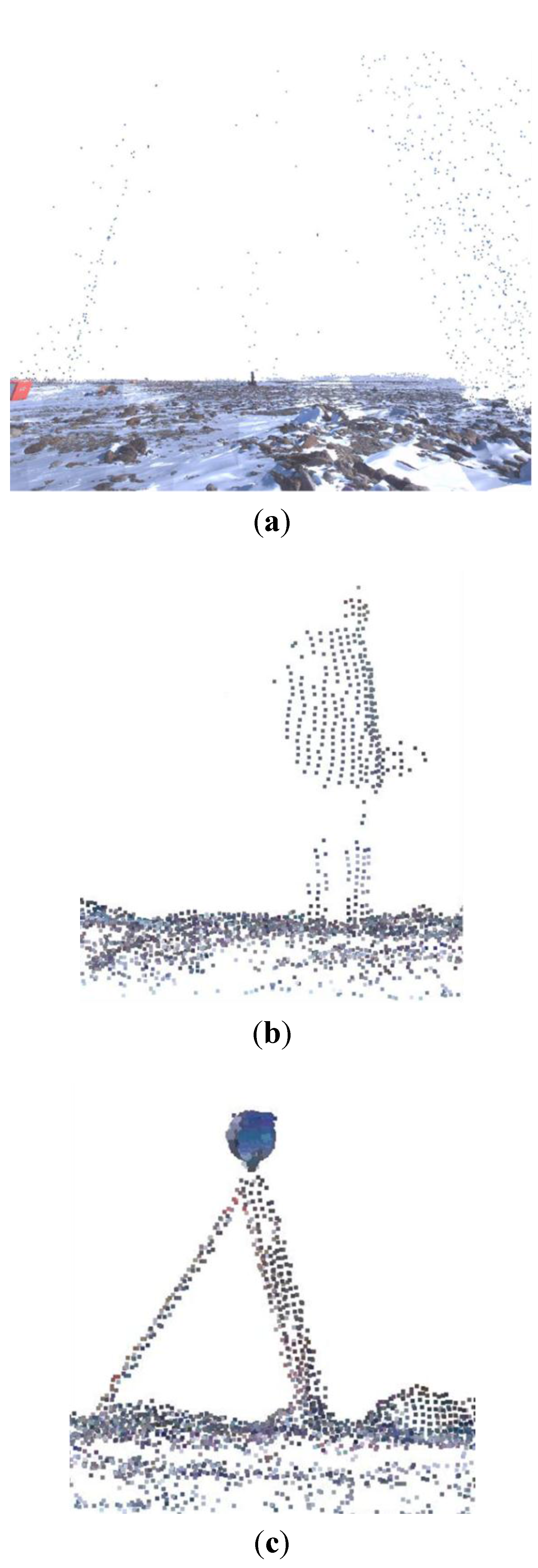
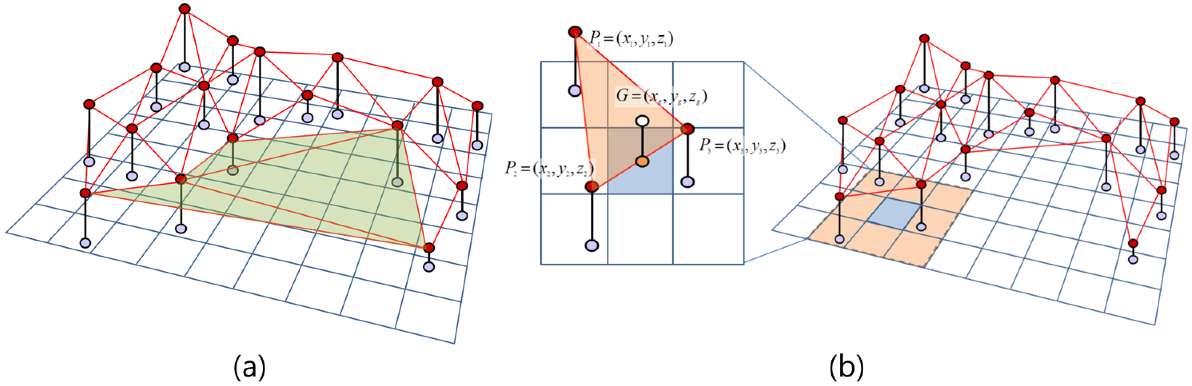
2.5. Digital Elevation Model (DEM) Generation
2.6. Accuracy Assessment
3. Results and Discussion
3.1. Data Acquisition
| Date | Activity | Date | Activity | Date | Activity |
|---|---|---|---|---|---|
| 02/04 | Installation of the base lines for GNSS observation | 02/07 | GNSS observation | 02/10 | Terrestrial LIDAR scanning |
| 02/05 | GNSS observation | 02/08 | 02/11 | ||
| 02/06 | Time delay due to bad weather condition | 02/09 | 02/12 | Check for the observed data and instruments |
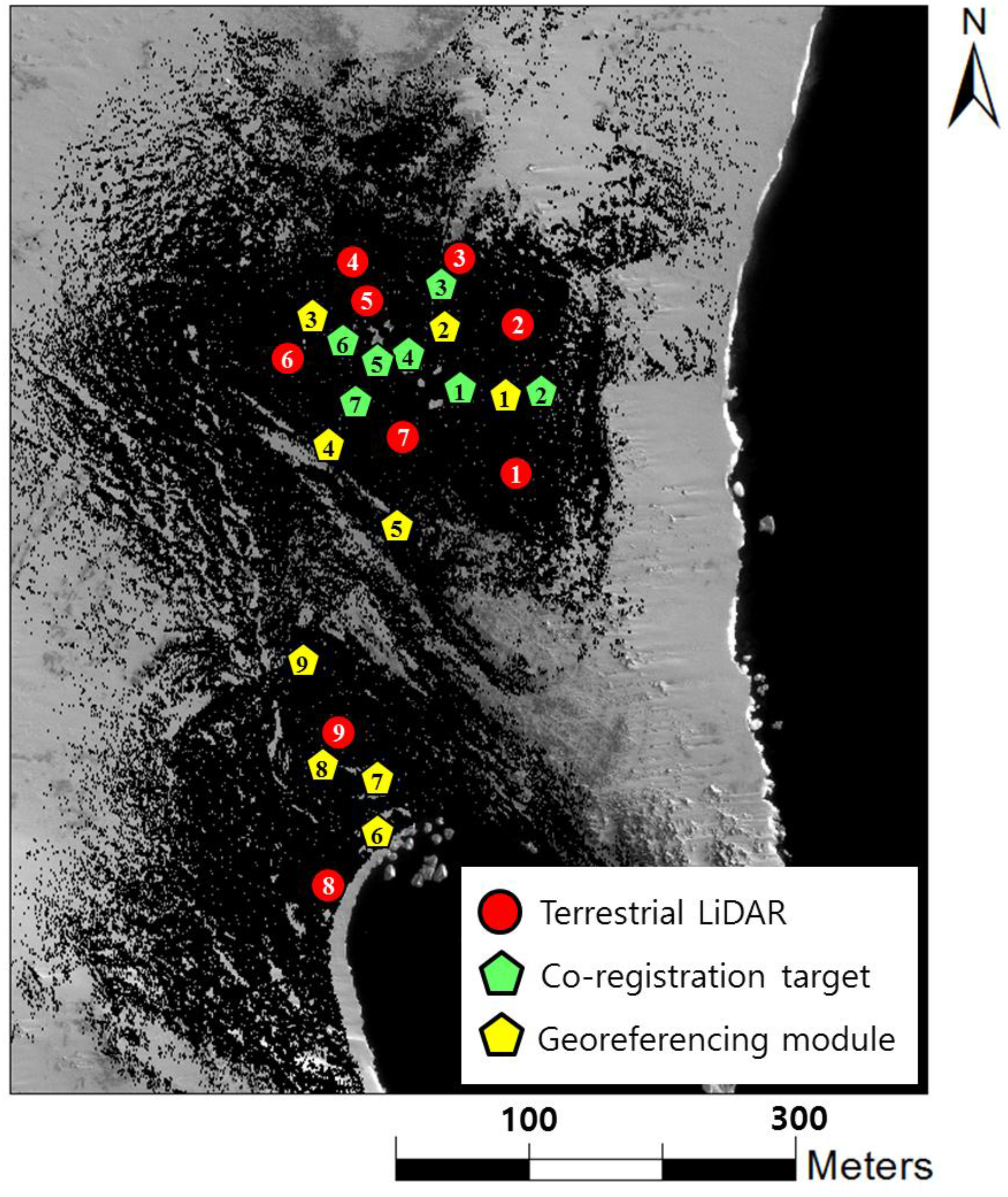
3.2. Co-Registration and Georeferencing
| Station | Distance (m) | Overlapped Area (m2) | Target ID | Co-Registration Precision (mm) | Georeferencing Precision (mm) | |
|---|---|---|---|---|---|---|
| Before Filtering | After Filtering | |||||
| st1–st2 | 126.223 | 15,907 | 1 c * | 3 | - | - |
| 1 g ** | 2 | 317 | 52 | |||
| 2 c | 3 | - | - | |||
| st2–st3 | 73.465 | 6522 | 1 c | 10 | - | - |
| 2 g | 4 | 1164 | Outlier ***** | |||
| 3 c | 8 | - | - | |||
| st3–st4 | 71.062 | 10,990 | 3 c,2 g, 4 c | X **** | - | - |
| ICP *** | 6 | - | - | |||
| st5–st6 | 77.581 | 10,447 | 5 c | 5 | - | - |
| 6 c | 3 | - | - | |||
| 3 g | 5 | 357 | 52 | |||
| st6–st7 | 115.115 | 23,264 | 5 c | 2 | - | - |
| 7 c | 3 | - | - | |||
| 4 g | 4 | 827 | Outlier | |||
| 5 g | X | - | - | |||
| st8–st9 ****** | 117.381 | 25,555 | 6 g | 14 | 62 | 62 |
| 7 g | 10 | 32 | 32 | |||
| 8 g | 5 | 29 | 29 | |||
| 9 g | X | - | - | |||
| RMSE | 5 | 398 | 45 | |||


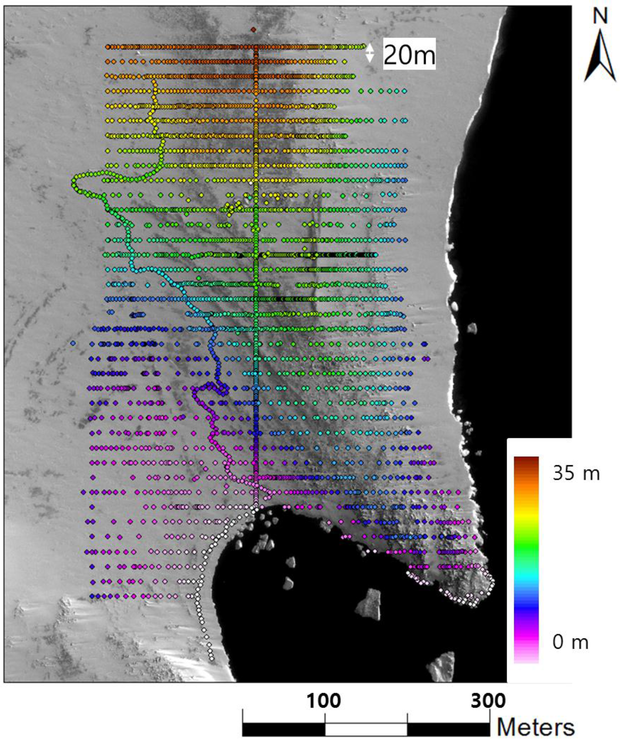
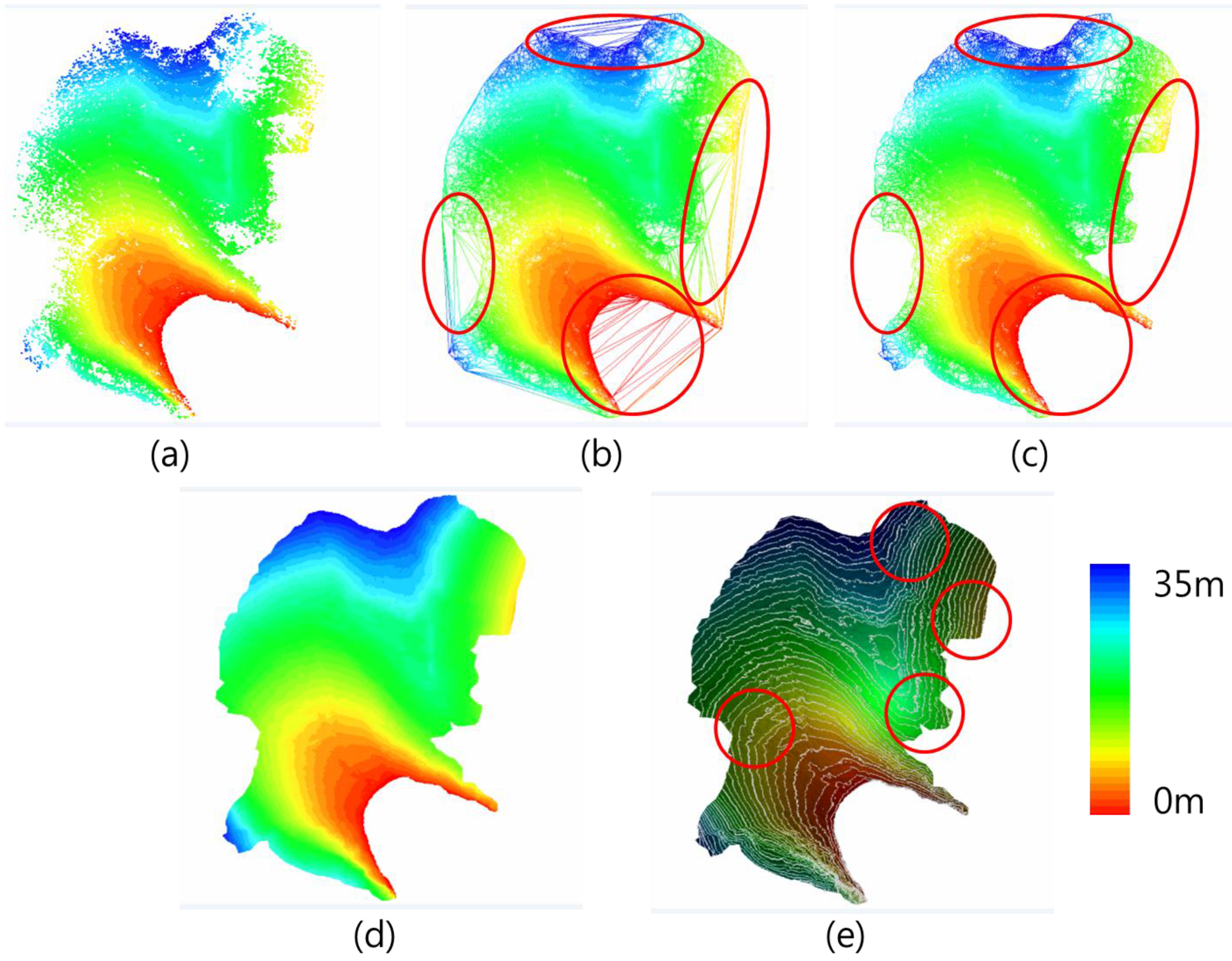
3.3. DEM Generation
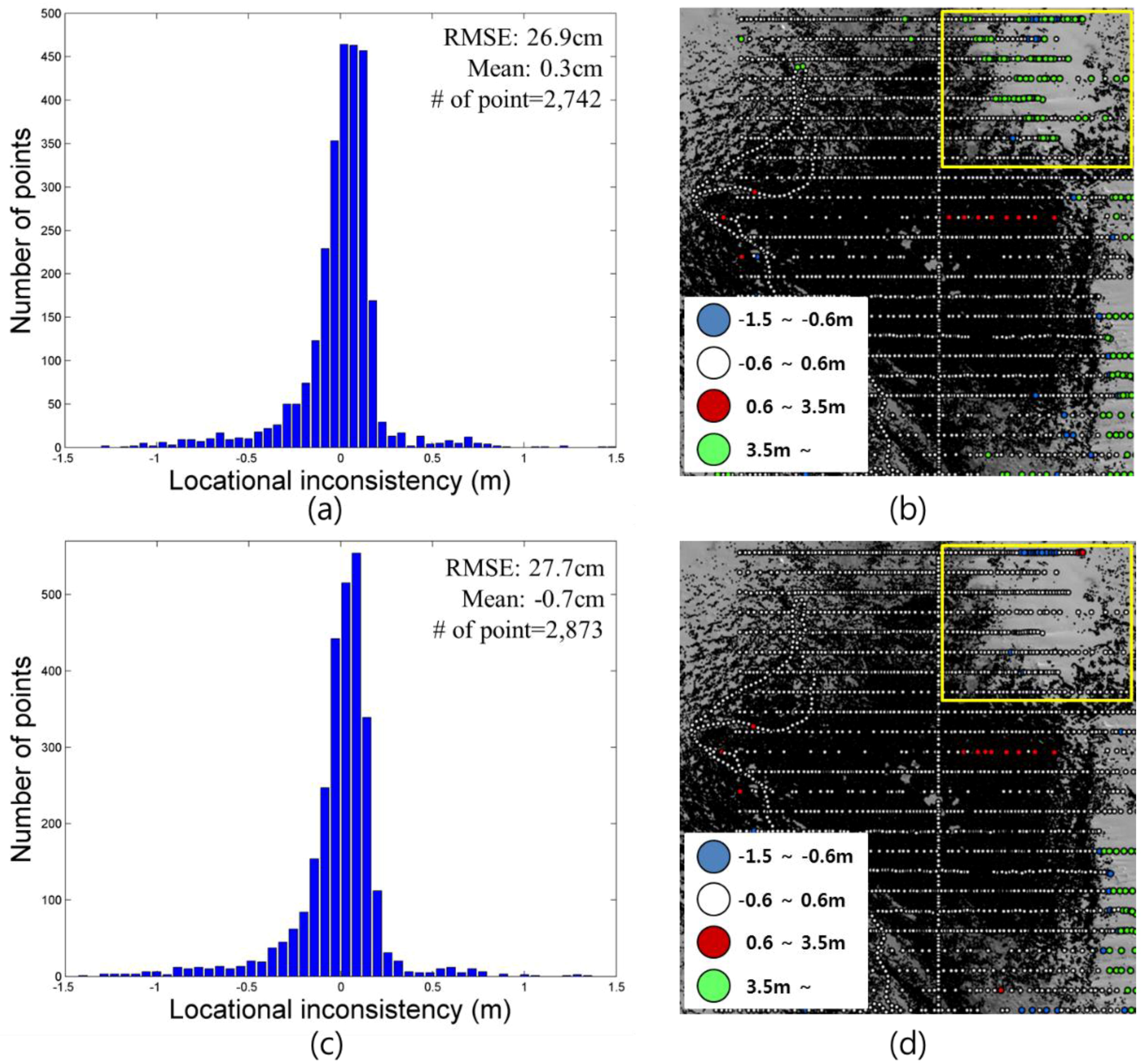
3.4. Accuracy Assessment

4. Conclusions
Acknowledgments
Author Contributions
Conflicts of Interest
References
- Payne, A.J.; Hunt, J.C.; Wingham, D.J. Evolution of the Antarctic ice sheet: New understanding and challenges. Philos. Trans. R. Soc. A Math. Phys. Eng. Sci. 2006, 364, 1867–1872. [Google Scholar] [CrossRef] [PubMed]
- Steig, E.J.; Schneider, D.P.; Rutherford, S.D.; Mann, M.E.; Comiso, J.C.; Shindell, D.T. Warming of the Antarctic ice-sheet surface since the 1957 international geophysical year. Nature 2009, 457, 459–462. [Google Scholar] [CrossRef] [PubMed]
- Wingham, D.J.; Ridout, A.J.; Scharroo, R.; Arthern, R.J.; Shum, C. Antarctic elevation change from 1992 to 1996. Science 1998, 282, 456–458. [Google Scholar] [CrossRef] [PubMed]
- Shepherd, A.; Wingham, D.; Rignot, E. Warm ocean is eroding West Antarctic ice sheet. Geophys. Res. Lett. 2004, 31. [Google Scholar] [CrossRef]
- Cuffey, K.M. A matter of firn. Science 2008, 320, 1596–1597. [Google Scholar] [CrossRef] [PubMed]
- Frey, H.; Paul, F. On the suitability of the SRTM DEM and ASTER GDEM for the compilation of topographic parameters in glacier inventories. Int. J. Appl. Earth Obs. Geoinf. 2012, 18, 480–490. [Google Scholar] [CrossRef]
- Bamber, J.L.; Rivera, A. A review of remote sensing methods for glacier mass balance determination. Glob. Planet. Chang. 2007, 59, 138–148. [Google Scholar] [CrossRef]
- Herzfeld, U.C.; Lingle, C.S.; Lee, L.-H. Geostatistical evaluation of satellite radar altimetry for high-resolution mapping of Lambert Glacier, Antarctica. Ann. Glaciol. 1993, 17, 77–85. [Google Scholar]
- Shepherd, A.; Wingham, D.J.; Mansley, J.A.; Corr, H.F. Inland thinning of pine island Glacier, West Antarctica. Science 2001, 291, 862–864. [Google Scholar] [CrossRef] [PubMed]
- Moholdt, G.; Nuth, C.; Hagen, J.O.; Kohler, J. Recent elevation changes of Svalbard glaciers derived from ICESat laser altimetry. Remote Sens. Environ. 2010, 114, 2756–2767. [Google Scholar] [CrossRef]
- Pritchard, H.; Ligtenberg, S.; Fricker, H.; Vaughan, D.; Van den Broeke, M.; Padman, L. Antarctic ice-sheet loss driven by basal melting of ice shelves. Nature 2012, 484, 502–505. [Google Scholar] [CrossRef] [PubMed]
- Rignot, E.; Jacobs, S.; Mouginot, J.; Scheuchl, B. Ice-shelf melting around Antarctica. Science 2013, 341, 266–270. [Google Scholar] [CrossRef] [PubMed]
- Sohn, H.-G.; Jezek, K. Mapping ice sheet margins from ERS-1 SAR and SPOT imagery. Int. J. Remote Sens. 1999, 20, 3201–3216. [Google Scholar] [CrossRef]
- Rosen, P.A.; Hensley, S.; Joughin, I.R.; Li, F.K.; Madsen, S.N.; Rodriguez, E.; Goldstein, R.M. Synthetic aperture radar interferometry. IEEE Proc. 2000, 88, 333–382. [Google Scholar] [CrossRef]
- Paul, F.; Huggel, C.; Kääb, A. Combining satellite multispectral image data and a digital elevation model for mapping debris-covered glaciers. Remote Sens. Environ. 2004, 89, 510–518. [Google Scholar] [CrossRef]
- Kääb, A. Glacier volume changes using ASTER satellite stereo and ICESat GLAS laser altimetry. A test study on Edgeøya, Eastern Svalbard. IEEE Trans. Geosci. Remote Sens. 2008, 46, 2823–2830. [Google Scholar] [CrossRef]
- Cook, A.; Murray, T.; Luckman, A.; Vaughan, D.; Barrand, N. A new 100-m digital elevation model of the Antarctic Peninsula derived from ASTER Global DEM: Methods and accuracy assessment. Earth Syst. Sci. Data 2012, 4, 129–142. [Google Scholar] [CrossRef]
- Bouin, M.N.; Vigny, C. New constraints on Antarctic plate motion and deformation from GPS data. J. Geophys. Res. Solid Earth 2000, 105, 28279–28293. [Google Scholar] [CrossRef]
- Dietrich, R.; Rülke, A.; Ihde, J.; Lindner, K.; Miller, H.; Niemeier, W.; Schenke, H.-W.; Seeber, G. Plate kinematics and deformation status of the Antarctic Peninsula based on GPS. Glob. Planet. Chang. 2004, 42, 313–321. [Google Scholar] [CrossRef]
- Donnellan, A.; Luyendyk, B.P. GPS evidence for a coherent Antarctic plate and for postglacial rebound in Marie Byrd Land. Glob. Planet. Chang. 2004, 42, 305–311. [Google Scholar] [CrossRef]
- Zanutta, A.; Vittuari, L.; Gandolfi, S. Geodetic GPS-based analysis of recent crustal motions in Victoria Land (Antarctica). Glob. Planet. Chang. 2008, 62, 115–131. [Google Scholar] [CrossRef]
- Nilsson, M. Estimation of tree heights and stand volume using an airborne LIDAR system. Remote Sens. Environ. 1996, 56, 1–7. [Google Scholar] [CrossRef]
- Popescu, S.C.; Wynne, R.H.; Nelson, R.F. Measuring individual tree crown diameter with LIDAR and assessing its influence on estimating forest volume and biomass. Can. J. Remote Sens. 2003, 29, 564–577. [Google Scholar] [CrossRef]
- Hong, S.H.; Cho, H.S.; Kim, N.H.; Sohn, H.G. 3D indoor modeling based on terrestrial laser scanning. J. Korean Soc. Civ. Eng. 2015, 35, 525–531. [Google Scholar] [CrossRef]
- Chehata, N.; Guo, L.; Mallet, C. Airborne LIDAR feature selection for urban classification using random forests. Int. Arch. Photogramm. Remote Sens. Spat. Inf. Sci. 2009, 38, 207–212. [Google Scholar]
- Yu, B.; Liu, H.; Wu, J.; Hu, Y.; Zhang, L. Automated derivation of urban building density information using airborne LIDAR data and object-based method. Landsc. Urban Plan. 2010, 98, 210–219. [Google Scholar] [CrossRef]
- Jones, L. Monitoring landslides in hazardous terrain using terrestrial LIDAR: An example from Montserrat. Q. J. Eng. Geol. Hydrogeol. 2006, 39, 371–373. [Google Scholar] [CrossRef]
- Wang, Z.; Li, H.; Wu, L. Geodesics-based topographical feature extraction from airborne LIDAR data for disaster management. In Proceedings of the 18th International Conference on Geoinformatics, Beijing, China, 18–20 June 2010; pp. 1–5.
- Jaboyedoff, M.; Oppikofer, T.; Abellán, A.; Derron, M.-H.; Loye, A.; Metzger, R.; Pedrazzini, A. Use of LIDAR in landslide investigations: A review. Nat. Hazards 2012, 61, 5–28. [Google Scholar] [CrossRef]
- Woolard, J.W.; Colby, J.D. Spatial characterization, resolution, and volumetric change of coastal dunes using airborne LIDAR: Cape Hatteras, North Carolina. Geomorphology 2002, 48, 269–287. [Google Scholar] [CrossRef]
- Arnold, N.; Rees, W.; Devereux, B.; Amable, G. Evaluating the potential of high-resolution airborne LIDAR data in glaciology. Int. J. Remote Sens. 2006, 27, 1233–1251. [Google Scholar] [CrossRef]
- Chen, Q. Airborne LIDAR data processing and information extraction. Photogramm. Eng. Remote Sens. 2007, 73, 109–112. [Google Scholar]
- Roering, J.J.; Stimely, L.L.; Mackey, B.H.; Schmidt, D.A. Using DInSAR, airborne LIDAR, and archival air photos to quantify landsliding and sediment transport. Geophys. Res. Lett. 2009, 36. [Google Scholar] [CrossRef]
- Liu, X. Airborne LIDAR for DEM generation: Some critical issues. Prog. Phys. Geograph. 2008, 32, 31–49. [Google Scholar]
- Pope, A.; Willis, I.; Rees, W.; Arnold, N.; Pálsson, F. Combining airborne LIDAR and landsat ETM+ data with photoclinometry to produce a digital elevation model for Langjökull, Iceland. Int. J. Remote Sens. 2013, 34, 1005–1025. [Google Scholar] [CrossRef]
- Slob, S.; Hack, R. 3D terrestrial laser scanning as a new field measurement and monitoring technique. In Engineering Geology for Infrastructure Planning in Europe; Springer: Berlin, Germany, 2004; pp. 179–189. [Google Scholar]
- Prokop, A. Assessing the applicability of terrestrial laser scanning for spatial snow depth measurements. Cold Reg. Sci. Technol. 2008, 54, 155–163. [Google Scholar] [CrossRef]
- Entwistle, J.; McCaffrey, K.; Abrahams, P. Three-dimensional (3D) visualisation: The application of terrestrial laser scanning in the investigation of historical Scottish farming townships. J. Archaeol. Sci. 2009, 36, 860–866. [Google Scholar] [CrossRef]
- Ergun, B. A novel 3D geometric object filtering function for application in indoor area with terrestrial laser scanning data. Opt. Laser Technol. 2010, 42, 799–804. [Google Scholar] [CrossRef]
- Abellán, A.; Oppikofer, T.; Jaboyedoff, M.; Rosser, N.J.; Lim, M.; Lato, M.J. Terrestrial laser scanning of rock slope instabilities. Earth Surf. Proc. Landf. 2014, 39, 80–97. [Google Scholar] [CrossRef]
- Reshetyuk, Y. Investigation and Calibration of Pulsed Time-Of-Flight Terrestrial Laser Scanners. Ph.D. Thesis, Royal Institute of Technology (KTH), Stockholm, Sweden, October 2006. [Google Scholar]
- Abate, D.; Pierattini, S.; Fasani, G.B. LIDAR in extreme environment: Surveying in Antarctica. ISPRS Ann. Photogramm. Remote Sens. Spat. Inf. Sci. 2013, 1, 1–6. [Google Scholar] [CrossRef]
- GSA BIM Guide For 3D Imaging. Available online: http://www.gsa.gov/portal/mediaId/226819/fileName/GSA_BIM_Guide_Series_03.action (accessed on 28 January 2015).
- Mitas, L.; Mitasova, H. Spatial interpolation. In Geographical Information Systems: Principles and Technical Issues; Longley, P.A., Goodchild, M., Maguire, D., Rhind, D.W., Eds.; John Wiley & Sons, Inc.: New York, NY, USA, 1999; Volume 1, pp. 481–492. [Google Scholar]
- Akima, H. A method of bivariate interpolation and smooth surface fitting for irregularly distributed data points. ACM Trans. Math. Softw. 1978, 4, 148–159. [Google Scholar] [CrossRef]
- Leica Geosystems. Datasheet of Leica ScanStation C10. Available online: http://hds.leica-geosystems.com/downloads123/hds/hds/ScanStation%20C10/brochures-datasheet/Leica_ScanStation_C10_DS_en.pdf (accessed on 28 January 2015).
- Ingensand, H. Metrological aspects in terrestrial laser-scanning technology. In Proceedings of the 3rd IAG/12th FIG symposium, Baden, Austria, 22–24 May 2006.
- Schulz, T. Calibration of A Terrestrial Laser Scanner for Engineering Geodesy. Ph.D. Thesis, ETH Zurich, Zurich, Switzerland, 2007. [Google Scholar]
- Chris Cothrun. The Technical Side: Dual Axis Compensators. Available online: http://www.krcmar.ca/sites/default/files/1995_Spring_Dual%20Axis%20Compensators_1.pdf (accessed on 20 August 2015).
- Becerik-Gerber, B.; Jazizadeh, F.; Kavulya, G.; Calis, G. Assessment of target types and layouts in 3D laser scanning for registration accuracy. Autom. Constr. 2011, 20, 649–658. [Google Scholar] [CrossRef]
- Jaw, J.J.; Chuang, T.Y. Registration of ground-based LIDAR point clouds by means of 3D line features. J. Chin. Inst. Eng. 2008, 31, 1031–1045. [Google Scholar] [CrossRef]
- Besl, P.J.; McKay, N.D. A method for registration of 3-D shapes. IEEE Trans. Patt. Anal. Mach. Intell. 1992, 14, 239–256. [Google Scholar] [CrossRef]
- Rusinkiewicz, S.; Levoy, M. Efficient variants of the ICP algorithm. In Proceedings of the 3th International Conference on 3D Digital Imaging and Modeling, Quebec City, QC, Canada, 28 May –1 June 2001; pp. 145–152.
- UNAVCO. UNAVCO TLS Target. Available online: http://facility.unavco.org/kb/questions/739/UNAVCO+TLS+Target (accessed on 20 August 2015).
- Gili, J.A.; Corominas, J.; Rius, J. Using global positioning system techniques in landslide monitoring. Eng. Geol. 2000, 55, 167–192. [Google Scholar] [CrossRef]
- Schloderer, G.; Bingham, M.; Awange, J.L.; Fleming, K.M. Application of GNSS-RTK derived topographical maps for rapid environmental monitoring: A case study of Jack Finnery Lake (Perth, Australia). Environ. Monit. Assess. 2011, 180, 147–161. [Google Scholar] [CrossRef] [PubMed]
© 2015 by the authors; licensee MDPI, Basel, Switzerland. This article is an open access article distributed under the terms and conditions of the Creative Commons Attribution license (http://creativecommons.org/licenses/by/4.0/).
Share and Cite
Cho, H.; Hong, S.; Kim, S.; Park, H.; Park, I.; Sohn, H.-G. Application of a Terrestrial LIDAR System for Elevation Mapping in Terra Nova Bay, Antarctica. Sensors 2015, 15, 23514-23535. https://doi.org/10.3390/s150923514
Cho H, Hong S, Kim S, Park H, Park I, Sohn H-G. Application of a Terrestrial LIDAR System for Elevation Mapping in Terra Nova Bay, Antarctica. Sensors. 2015; 15(9):23514-23535. https://doi.org/10.3390/s150923514
Chicago/Turabian StyleCho, Hyoungsig, Seunghwan Hong, Sangmin Kim, Hyokeun Park, Ilsuk Park, and Hong-Gyoo Sohn. 2015. "Application of a Terrestrial LIDAR System for Elevation Mapping in Terra Nova Bay, Antarctica" Sensors 15, no. 9: 23514-23535. https://doi.org/10.3390/s150923514
APA StyleCho, H., Hong, S., Kim, S., Park, H., Park, I., & Sohn, H.-G. (2015). Application of a Terrestrial LIDAR System for Elevation Mapping in Terra Nova Bay, Antarctica. Sensors, 15(9), 23514-23535. https://doi.org/10.3390/s150923514