
Illumination and Reflectance Estimation with its Application in Foreground Detection

Abstract
:1. Introduction
2. Methodology
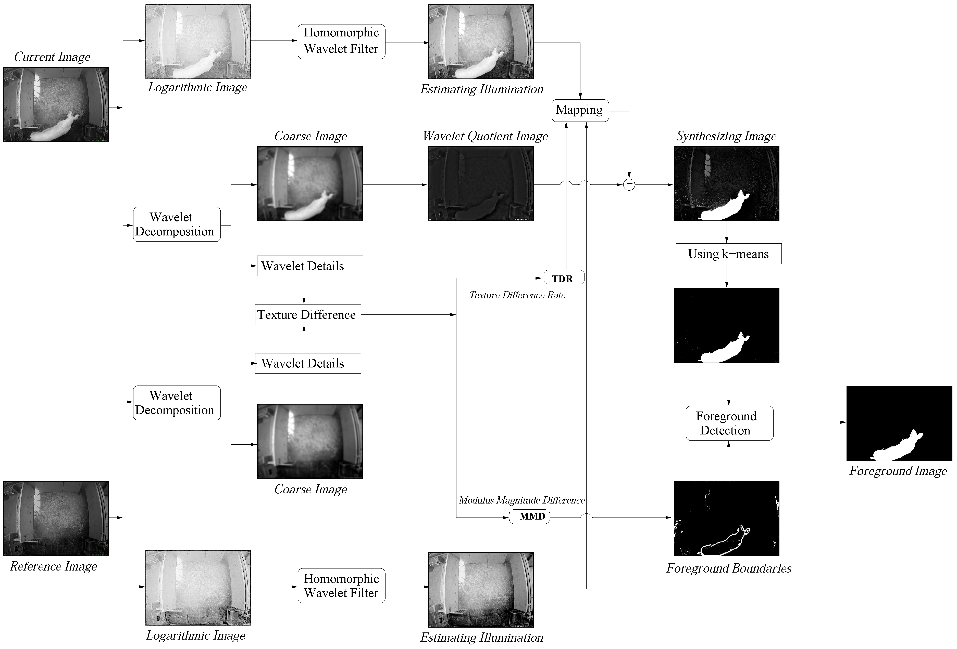
2.1. Homomorphic Wavelet Filter

2.2. Wavelet-Quotient Image Model
2.3. Texture Difference Measure
2.4. The Synthesizing Image
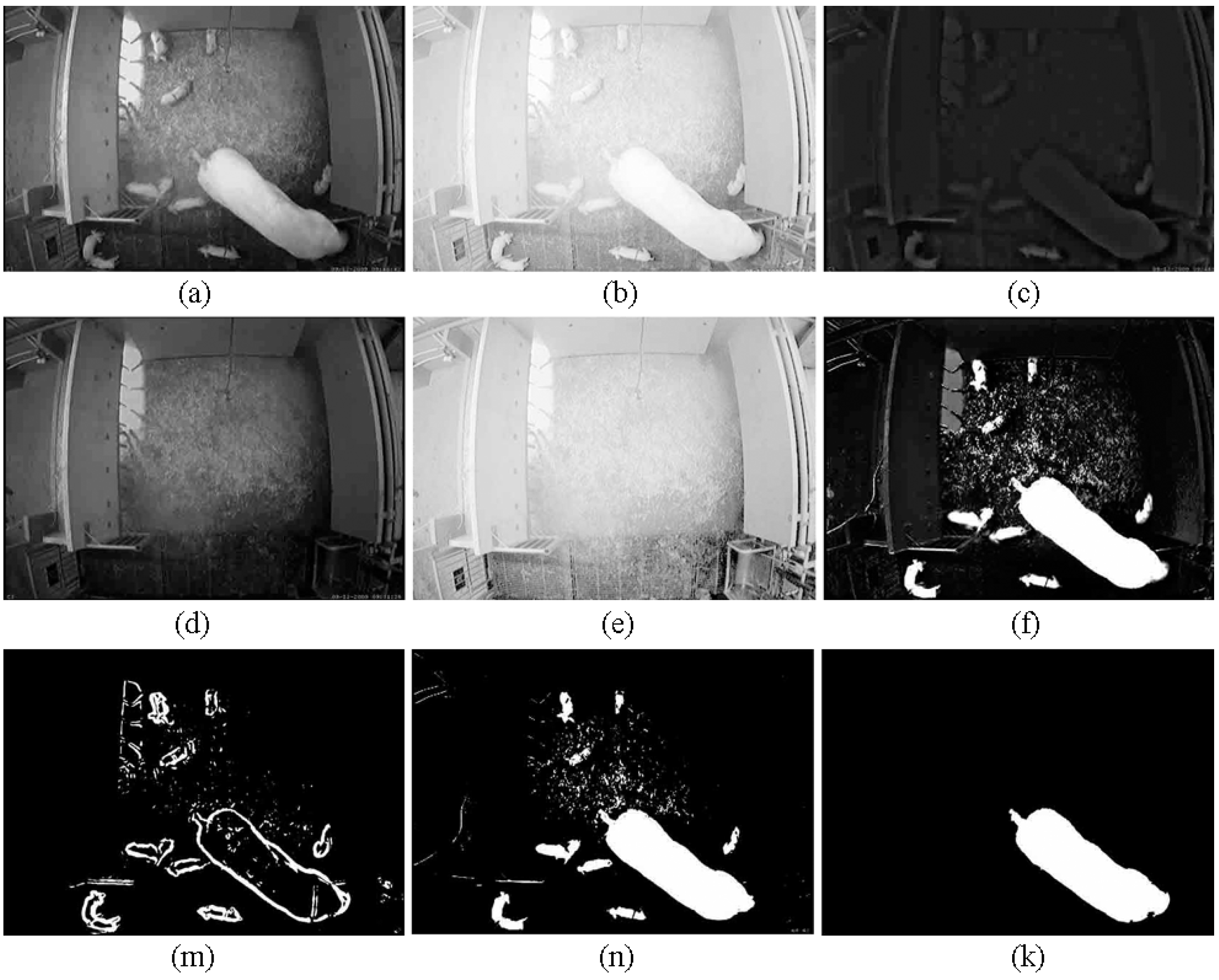
2.5. Foreground Detection
- A morphological close filtering is performed on the image using a circular structuring element of 3-pixel diameter to fill the gaps and smooth out the edges.
- To separate the piglets and the sow, we subtract the two images: . After subtracting, the piglets and the sow are separated if they connect together. We remove the small areas in the image , so the piglets are eliminated. Then, the area of the foreground object, which is a total number of pixels of the sow in the image , is extracted.
- Now we combine the images and : . After combining, again, in order to eliminate the boundaries of the piglets, we remove the small areas in the image .
- The connected components algorithm and some other post-processing operations are performed in the combined image to extract the shape of the sow.
3. The Proposed Algorithm

| 0. Input the reference image (i.e., background); |
| Estimate the illumination of the reference image by using HWF (see Figure 1); |
| Estimate the coarse image and wavelet details of the reference image by using Equation (2); |
| 1. repeat |
| 2. Input the current image; |
| 3. Estimate the illumination of the current image by using HWF (see Figure 1); |
| 4. Estimate the coarse image and wavelet details of the current image by using Equation (2); |
| 5. Estimate the reflectance of the current image by using WQI (i.e., Equation (10)); |
| 6. Synthesize an image by using Equation (15), the estimated illumination and reflectance of the current image and the estimated illumination of the reference image are used in the function; |
| 7. Estimate the foreground objects based on the synthesizing image by using Equation (18); |
| 8. Estimate the boundaries of the foreground objects by using Equation (19); |
| 9. Detect the sow based on the foreground (i.e., step 7) and boundary (i.e., step 8) images, the approach is described in Section 2.5. |
| 10. end |
4. Material Used in this Study
4.1. Training Data
4.2. Test Data
4.3. Evaluation Criteria
- Criteria for original images:We manually evaluated the area of the sow for all original images in the test data and some original images in the training data. The evaluated area was used to compare with the corresponding shape of the sow in the segmented binary image.To demonstrate the segmentation efficiency under different illumination conditions, the original images were evaluated within about 1 hour in the two training data sets after the sow and piglets went into the pen, since the two periods contained different light conditions that were manually made. The original images were manually classified into two illumination levels: Normal and Change. The Normal level means that the lights were not or slowly changed and the Change level means that the lights were changed (i.e., the lights were switched on or off at that moment).
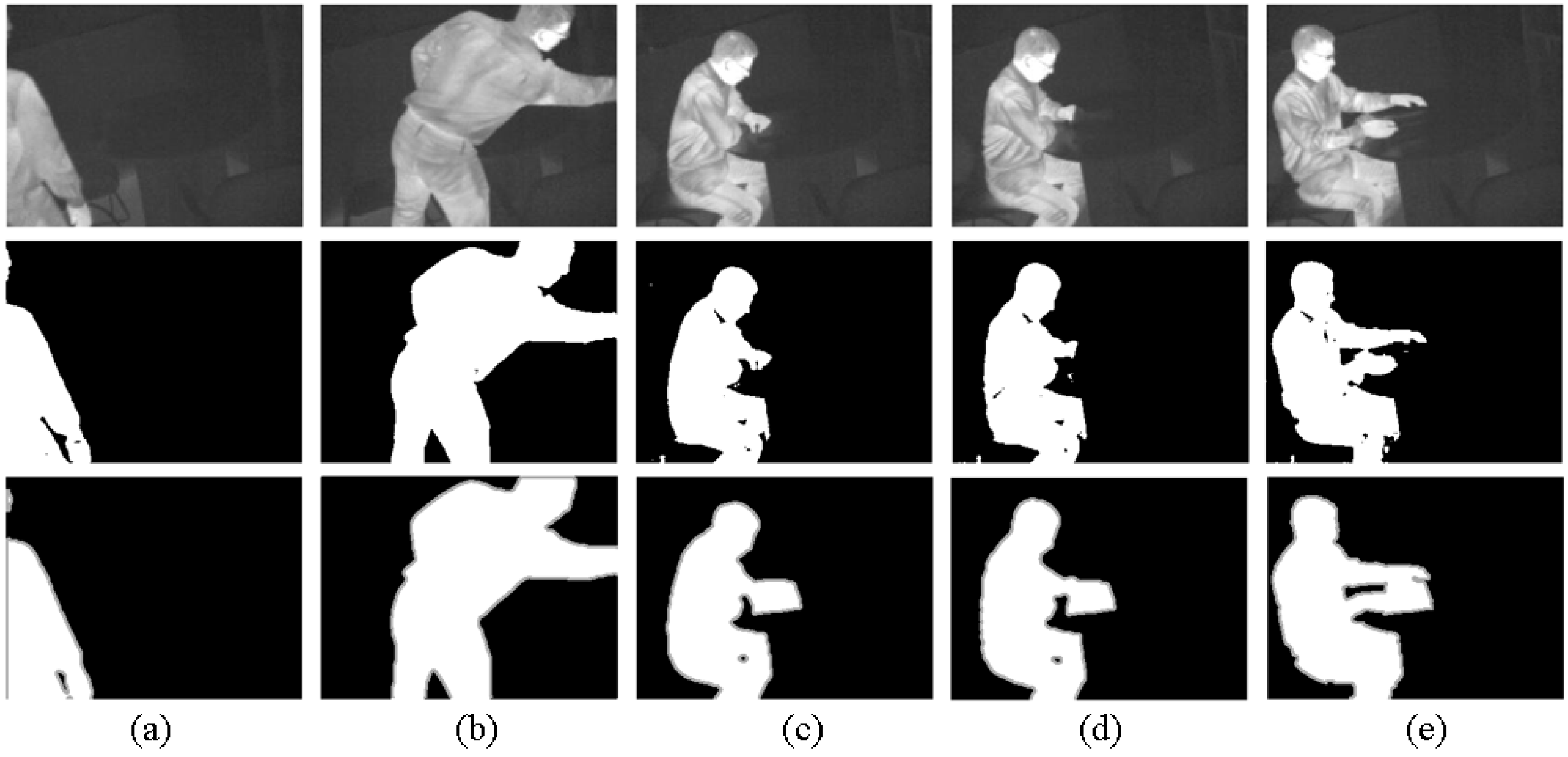
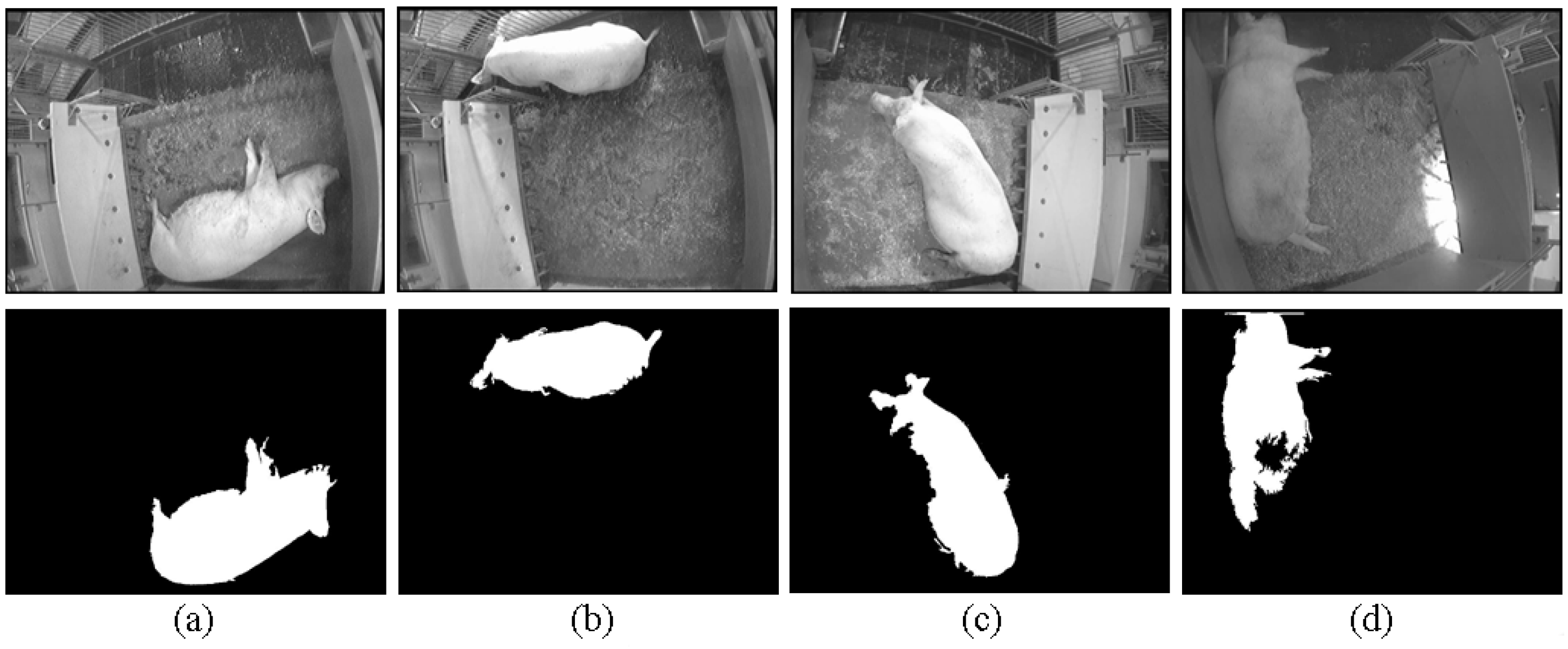
- Criteria for segmented images:The segmented images were visually evaluated and classified into three scale groups. (1) Full Segmentation (FS): the shape of the sow was segmented over 90% of the manually evaluated area; (2) Partial Segmentation (PS): the shape of the sow was segmented between 80% and 90% of the manually evaluated area; (3) Cannot Segment (CNS): (a) there were two or more separated regions; (b) there were many false foreground pixels in the segmented image; (c) the shape of the sow was segmented below 80% of the manually evaluated area.The classification was based on a comparison (i.e., ratio) between the manually evaluated area and the corresponding area of the shape of the sow in the segmented image. The corresponding segmented images that represent the three scale groups are shown in Figure 7.
5. Experimental Results
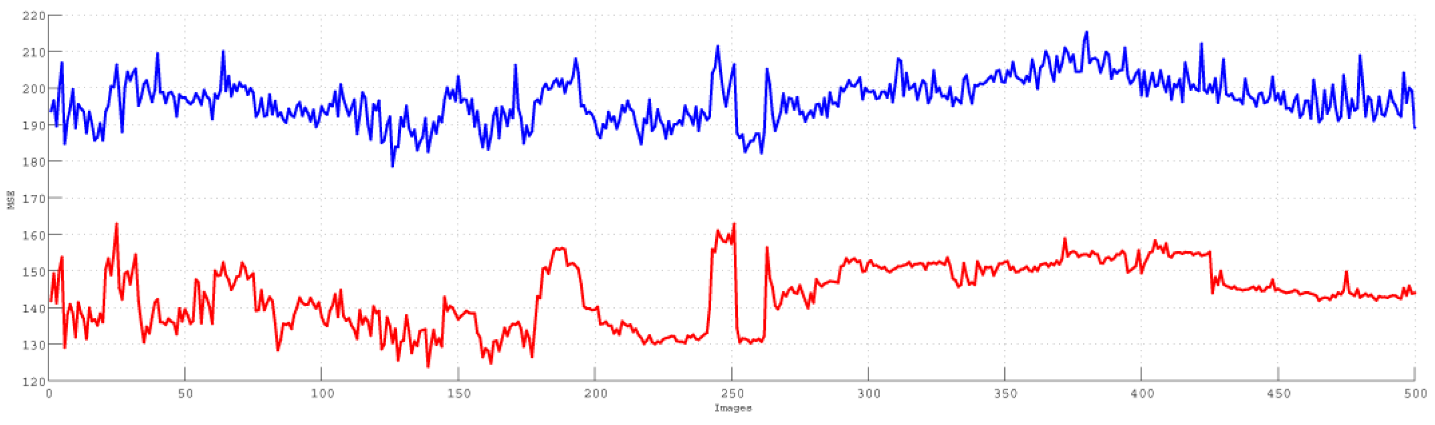
5.1. HWF Evaluation

5.2. WQI Evaluation
5.3. Detection Evaluation
5.3.1. Qualitative Evaluation
5.3.2. Quantitative Evaluation
| Data Set | Total Images | FS | PS | CNS | ||||||
|---|---|---|---|---|---|---|---|---|---|---|
| N | % | N | % | N | % | |||||
| 1 | 1435 | 1372 | 95.61 | 43 | 2.99 | 20 | 1.39 | |||
| 2 | 1434 | 1370 | 95.54 | 46 | 3.21 | 18 | 1.26 | |||
| 3 | 1437 | 1369 | 95.27 | 51 | 3.55 | 17 | 1.18 | |||
| 4 | 1435 | 1374 | 95.75 | 42 | 2.93 | 19 | 1.32 | |||
| 5 | 1436 | 1375 | 95.75 | 41 | 2.86 | 20 | 1.39 | |||
| 6 | 1435 | 1367 | 95.26 | 43 | 2.30 | 25 | 1.74 | |||
| 7 | 1436 | 1369 | 95.33 | 45 | 3.13 | 22 | 1.53 | |||
| 8 | 1433 | 1372 | 95.74 | 41 | 2.86 | 20 | 1.40 | |||
| 9 | 1438 | 1375 | 95.19 | 48 | 3.34 | 15 | 1.04 | |||
| 10 | 1435 | 1369 | 95.40 | 43 | 3.00 | 23 | 1.63 | |||
| Average | 95.48 | 3.02 | 1.39 | |||||||
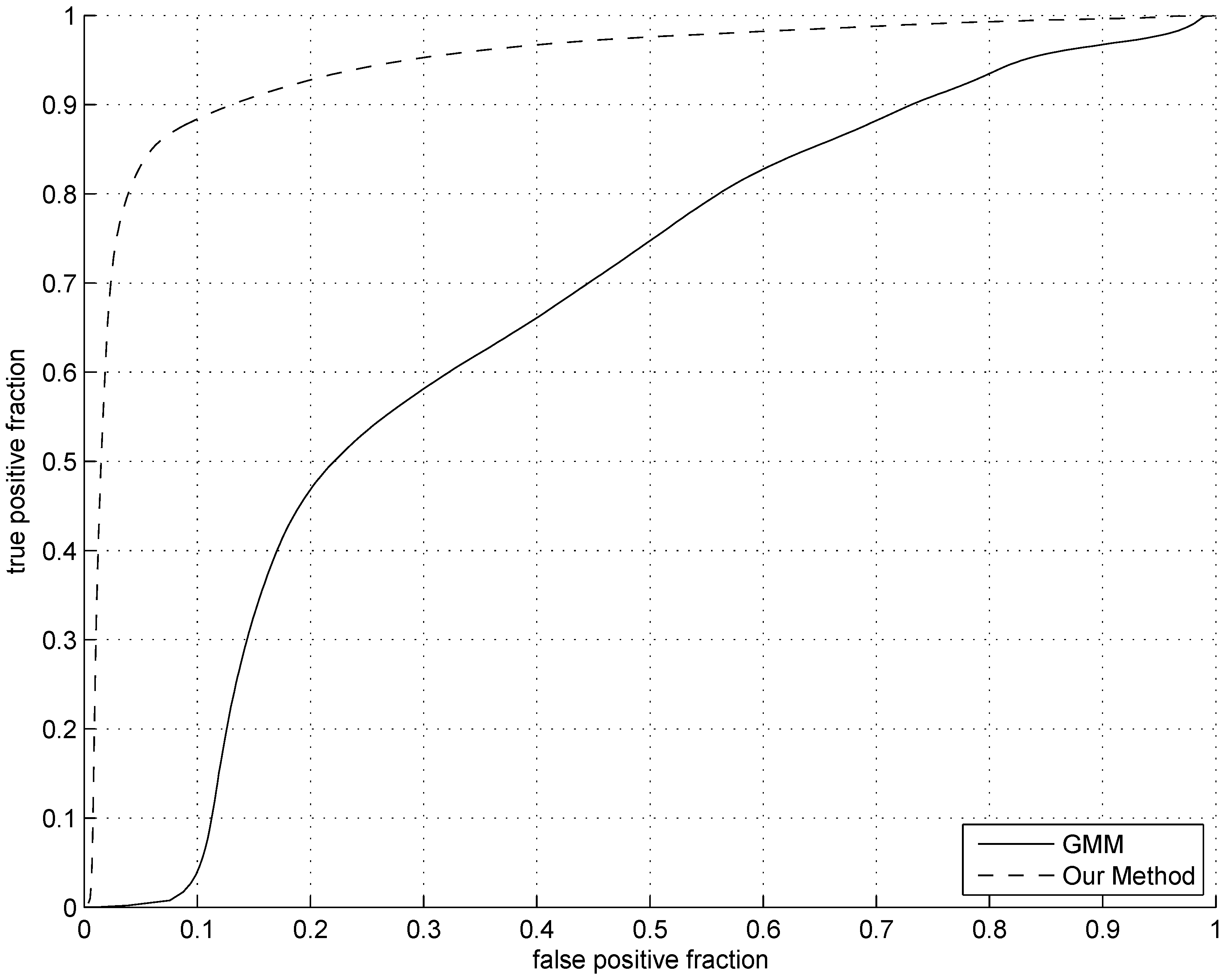
5.4. Comparison
| Illumination | N | Our Algorithm | GMM-Based Method | ||||||||||
|---|---|---|---|---|---|---|---|---|---|---|---|---|---|
| FS | PS | CNS | FS | PS | CNS | ||||||||
| Level | N | % | N | % | N | % | N | % | N | % | N | % | |
| Normal | 594 | 589 | 99.15 | 4 | 0.67 | 0.17 | 0.27 | 544 | 91.58 | 42 | 7.07 | 8 | 1.34 |
| Change | 126 | 117 | 92.9 | 6 | 4.7 | 3 | 2.4 | 9 | 7.2 | 13 | 10.3 | 104 | 82.5 |

5.5. The Publicly Available Data

6. Conclusions
Acknowledgments
Author Contributions
Conflicts of Interest
References
- Piccardi, M. Background subtraction techniques: A review. In Proceedings of the IEEE International Conference on Systems, Man and Cybernetics, Orlando, FL, USA, 11–13 October 2004; pp. 3099–3104.
- Elhabian, S.; El-Sayed, K.; Ahmed, S. Moving object detection in spatial domain using background removal techniques-state-of-art. In Proceedings of the IEEE International Conference on Systems, Man and Cybernetics, Singapore, 12–15 October 2008; pp. 32–54.
- Bouwmans, T.; El Baf, F.; Vachon, B. Background Modeling Using Mixturqe of Gaussians for Foreground Detection—A Survey. Recent Patents Comput. Sci. 2008, 1, 219–237. [Google Scholar] [CrossRef]
- Bouwmans, T. Subspace learning for background modeling: A survey. Recent Patents Comput. Sci. 2009, 2, 223–234. [Google Scholar] [CrossRef]
- Bouwmans, T.; El Baf, F.; Vachon, B. Statistical Background Modeling for Foreground Detection: A Survey. In Handbook of Pattern Recognition and Computer Vision; World Scientific Publishing: Singapore, 2010; pp. 181–199. [Google Scholar]
- Bouwmans, T. Recent Advanced Statistical Background Modeling for Foreground Detection: A Systematic Survey. Recent Patents Comput. Sci. 2011, 4, 147–176. [Google Scholar]
- Brutzer, S.; Hoferlin, B.; Heidemann, G. Evaluation of background subtraction techniques for video surveillance. In Proceedings of the 2011 IEEE Conference on Computer Vision and Pattern Recognition, Providence, RI, USA, 20–25 June 2011; pp. 1937–1944.
- Li, L.; Huang, W.; Gu, I.; Tian, Q. Statistical Modeling of Complex Backgrounds for Foreground Object Detection. IEEE Trans. Image Process. 2004, 13, 1459–1472. [Google Scholar] [CrossRef] [PubMed]
- Cheng, F.; Chen, Y. Real time multiple objects tracking and identification based on discrete wavelet transform. J. Pattern Recognit. 2006, 39, 1126–1139. [Google Scholar] [CrossRef]
- Khare, M.; Srivastava, R.; Khare, A. Moving object segmentation in Daubechies complex wavelet domain. Signal Image Video Process. 2015, 9, 635–650. [Google Scholar] [CrossRef]
- Openheim, A.; Schafer, R.; Stockham, T.G., Jr. Nonlinear filtering of multiplied and convolved signals. IEEE Proc. 1968, 56, 1264–1291. [Google Scholar] [CrossRef]
- Chen, H.; Belhumeur, P.; Jacobs, D. In search of illumination invariants. In Proceedings of the IEEE Conference on Computer Vision and Pattern Recognition, Hilton Head Island, SC, USA, 13–15 June 2000; pp. 254–261.
- Gonzalez, R.C.; Wintz, P. Digital Image Processing; Addison-Wesley Publishing Company: Boston, MA, USA, 1993. [Google Scholar]
- Singh, H.; Roman, C.; Pizarro, O.; Eustice, R.; Can, A. Towards high-resolution imaging from underwater vehicles. Int. J. Robot. Res. 2007, 26, 55–74. [Google Scholar] [CrossRef]
- Stainvas, I.; Lowe, D. A generative model for separating illumination and reflectance from images. J. Mach. Learn. Res. 2004, 4, 1499–1519. [Google Scholar]
- Toth, D.; Aach, T.; Metzler, V. Illumination-invariant change detection. In Proceedings of the 4th IEEE Southwest Symposium on Image Analysis and Interpretation, Austin, TX, USA, 2–4 April 2000; pp. 3–7.
- Mallat, S.; Zhong, S. Characterization of signals from multiscale edges. IEEE Trans. Pattern Anal. Mach. Intell. 1992, 14, 710–732. [Google Scholar] [CrossRef]
- Wang, H.; Li, S.; Wang, Y. Generalized quotient image. In Proceedings of the IEEE International Conference Computer Vision and Pattern Recognition, Washington, DC, USA, 27 June–2 July 2004; pp. 498–505.
- McFarlane, N.; Schofield, C. Segmentation and tracking of piglets in images. Mach. Vis. Appl. 1995, 8, 261–275. [Google Scholar] [CrossRef]
- Tillett, R.; Onyango, C.; Marchant, J. Using model-based image processing to track animal movements. Comput. Electron. Agric. 1997, 17, 249–261. [Google Scholar] [CrossRef]
- Hu, J.; Xin, H. Image-processing algorithms for behavior analysis of group-housed pigs. Behav. Res. Methods Instrum. Comput. 2000, 32, 72–85. [Google Scholar] [CrossRef] [PubMed]
- Perner, P. Motion tracking of animals for behavior analysis. In Proceedings of the 4th International Work Shop on VisualForm (IWVF-4); Springer Heidelberg: Berlin, Germany, 2001; pp. 779–786. [Google Scholar]
- Lind, N.; Vinther, M.; Hemmingsen, R.; Hansen, A. Validation of a digital video tracking system for recording pig locomotor behaviour. J. Neurosci. Methods 2005, 143, 123–132. [Google Scholar] [CrossRef] [PubMed]
- Shao, B.; Xin, H. A real-time computer vision assessment and control of thermal comfort for group-housedpigs. Comput. Electron. Agric. 2008, 62, 15–21. [Google Scholar] [CrossRef]
- Ahrendt, P.; Gregersen, T.; Karstoft, H. Development of a real-time computer vision system for tracking loose-housed pigs. Comput. Electron. Agric. 2011, 76, 169–174. [Google Scholar] [CrossRef]
- Guo, Y.; Zhu, W.; Jiao, P.; Chen, J. Foreground detection of group-housed pigs based on the combination of mixture of Gaussians using prediction mechanism and threshold segmentation. Biosyst. Eng. 2014, 125, 98–104. [Google Scholar] [CrossRef]
- Han, H.; Shan, S.; Chen, X.; Gao, W. Illumination transfer using homomorphic wavelet filtering and its application to light-insensitive face recognition. In Proceedings of the 8th IEEE International Conference on Automatic Face Gesture Recognition, Amsterdam, the Netherlands, 17–19 September 2008; pp. 1–6.
- Wang, H.; Li, S.Z.; Wang, Y. Face Recognition under Various Lighting Conditions by Self Quotient Image. In Proceedings of the 6th International Conference on Automatic Face and Gesture Recognition, Seoul, Korea, 17–19 May 2004.
- Shashua, A.; Riklin-Raviv, T. The quotient image: Classbased re-rendering and recognition with varying illuminations. IEEE Trans. Pattern Anal. Mach. Intell. 2001, 23, 129–139. [Google Scholar] [CrossRef]
- Perona, P.; Malik, J. Scale space and edge detection using anisotropic diffusion. In Proceedings of the IEEE Transactions on Pattern Analysis and Machine Intelligence, Miami Beach, FL, USA, 30 November–2 December 1987; pp. 16–22.
- Perona, P.; Malik, J. Scale space and edge detection using anisotropic diffusion. IEEE Trans. Pattern Anal. Mach. Intell. 1990, 12, 629–639. [Google Scholar] [CrossRef]
- Li, L.; Leung, M.K.H. Integrating intensity and texture differences for robust change detection. IEEE Trans. Image Process. 2002, 11, 105–112. [Google Scholar] [PubMed]
- MacQueen, J.B. Some Methods for classification and Analysis of Multivariate Observations. In Proceedings of 5th Berkeley Symposium on Mathematical Statistics and Probability; University of California Press: Oakland, CA, USA, 1967; pp. 281–297. [Google Scholar]
- Wippig, D.; Klauer, B. GPU-Based Translation-Invariant 2D Discrete Wavelet Transform for Image Processing. Int. J. Comput. 2011, 5, 226–234. [Google Scholar]
- Shafro, M. MSH-Video: Digital Video Surveillance System. Avalaible online: http://www.guard.lv/ (accessed on 23 April 2015).
- Zivkovic, Z.; van Der Heijden, F. Recursive unsupervised learning of finite mixture models. IEEE Trans. Pattern Recognit. Mach. Intell. 2004, 26, 651–656. [Google Scholar] [CrossRef] [PubMed]
- Padmavathi, G.; Subashini, P.; Muthu Kumar, M.; Kumar Thakur, S. Comparison of Filters Used for Underwater Image Pre-Processing. IJCSNS Int. J. Comput. Sci. Netw. Secur. 2011, 10, 58–65. [Google Scholar]
© 2015 by the authors; licensee MDPI, Basel, Switzerland. This article is an open access article distributed under the terms and conditions of the Creative Commons Attribution license (http://creativecommons.org/licenses/by/4.0/).
Share and Cite
Tu, G.J.; Karstoft, H.; Pedersen, L.J.; Jørgensen, E. Illumination and Reflectance Estimation with its Application in Foreground Detection. Sensors 2015, 15, 21407-21426. https://doi.org/10.3390/s150921407
Tu GJ, Karstoft H, Pedersen LJ, Jørgensen E. Illumination and Reflectance Estimation with its Application in Foreground Detection. Sensors. 2015; 15(9):21407-21426. https://doi.org/10.3390/s150921407
Chicago/Turabian StyleTu, Gang Jun, Henrik Karstoft, Lene Juul Pedersen, and Erik Jørgensen. 2015. "Illumination and Reflectance Estimation with its Application in Foreground Detection" Sensors 15, no. 9: 21407-21426. https://doi.org/10.3390/s150921407
APA StyleTu, G. J., Karstoft, H., Pedersen, L. J., & Jørgensen, E. (2015). Illumination and Reflectance Estimation with its Application in Foreground Detection. Sensors, 15(9), 21407-21426. https://doi.org/10.3390/s150921407