
Recognizing Banknote Fitness with a Visible Light One Dimensional Line Image Sensor


Abstract
:1. Introduction

| Category | Method | Advantages | Disadvantage | |
|---|---|---|---|---|
| Multiple sensor-based method | -Evaluating the five soiling levels of Euro banknotes by using various sensors [4]. | Using information by various sensors allows for the extraction of more discriminating features | -Focuses on analyzing the soiling property of the banknotes without proposing a solution for automatically classifying the fitness of banknotes [4]. | |
| -Denomination classification using visible and IR sensors [6]. | -Mainly focuses on denomination classification [6] and counterfeit banknote detection [13]. | |||
| -Detecting fake banknotes by CCD cameras with visible, UV, and IR lights [13]. | -Using multiple sensors leads to complexity in hardware implementation and an increase in processing time with multiple images from multiple sensors. | |||
| Single sensor-based method | Color sensor-based method | -Features are extracted from banknote images of various color channels [1,5]. -Detecting counterfeit Indian banknotes using features from HSV color space and neural network classifier [12]. | Using a single sensor causes simplicity in the algorithm and system implementation with reduced processing time | -Banknote images with multiple color channels must be acquired, and a large number of features based on many weak classifiers must be combined, thus reducing the processing speed [1,5]. -Mainly focuses on counterfeit banknote classification [12]. |
| Gray sensor-based method | Chinese banknote classification using neural network based on the features of gray-level histogram [7] -Fitness classification based on DWT and SVM (proposed method) | -Fast image acquisition by single gray sensor with less memory usage | -Mainly focuses on banknote classification [7]. -Additional procedure for SVM training is required (proposed method) | |
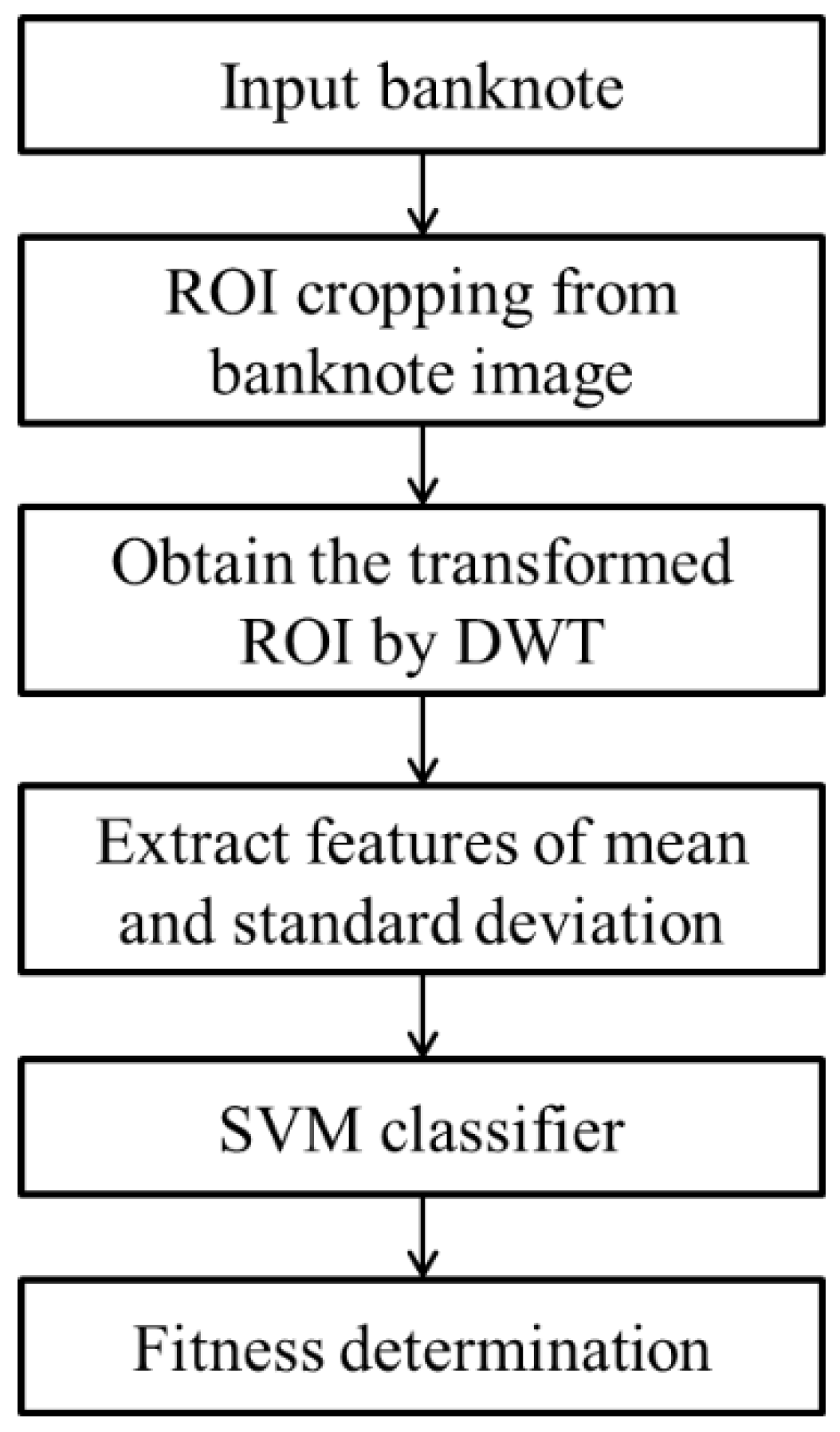
2. Proposed Method
2.1. Overview of the Proposed Method

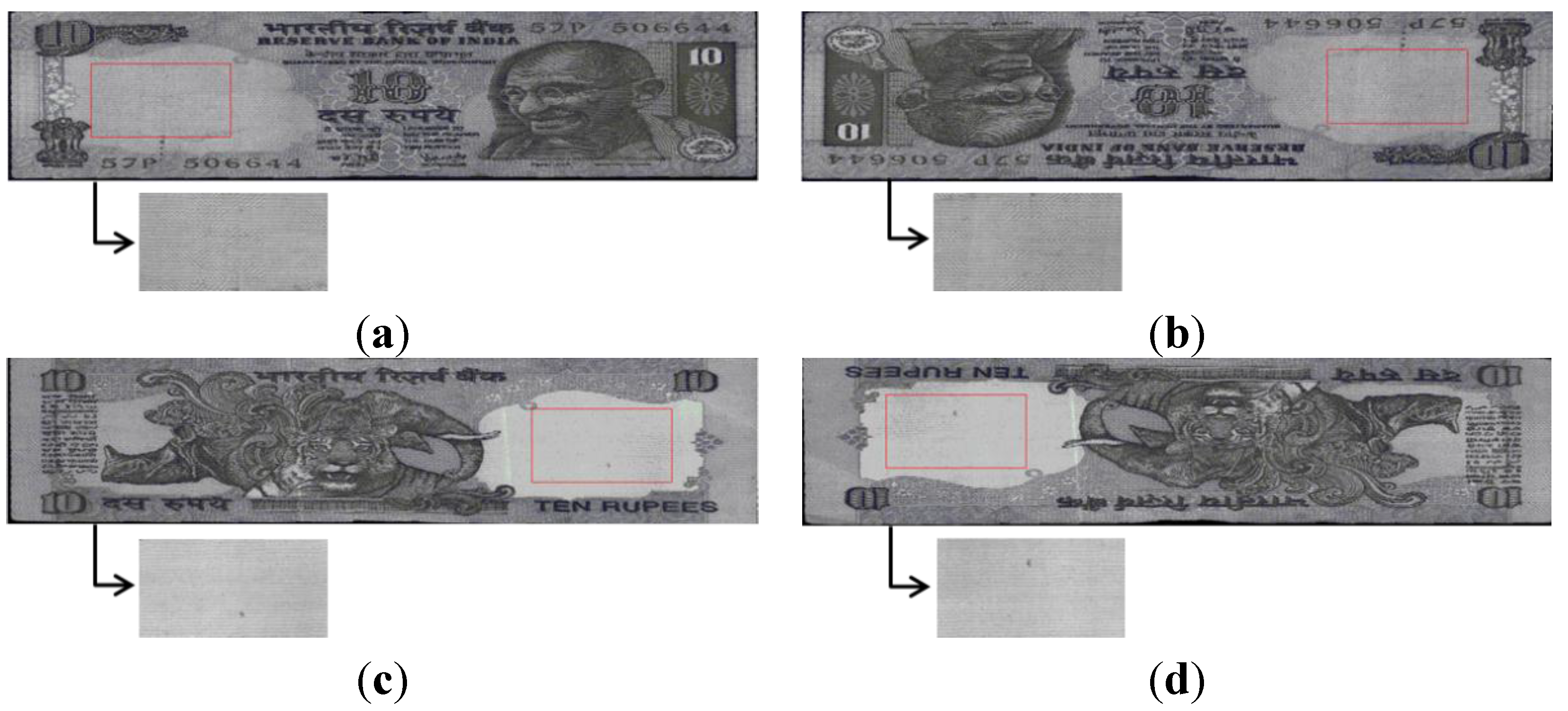
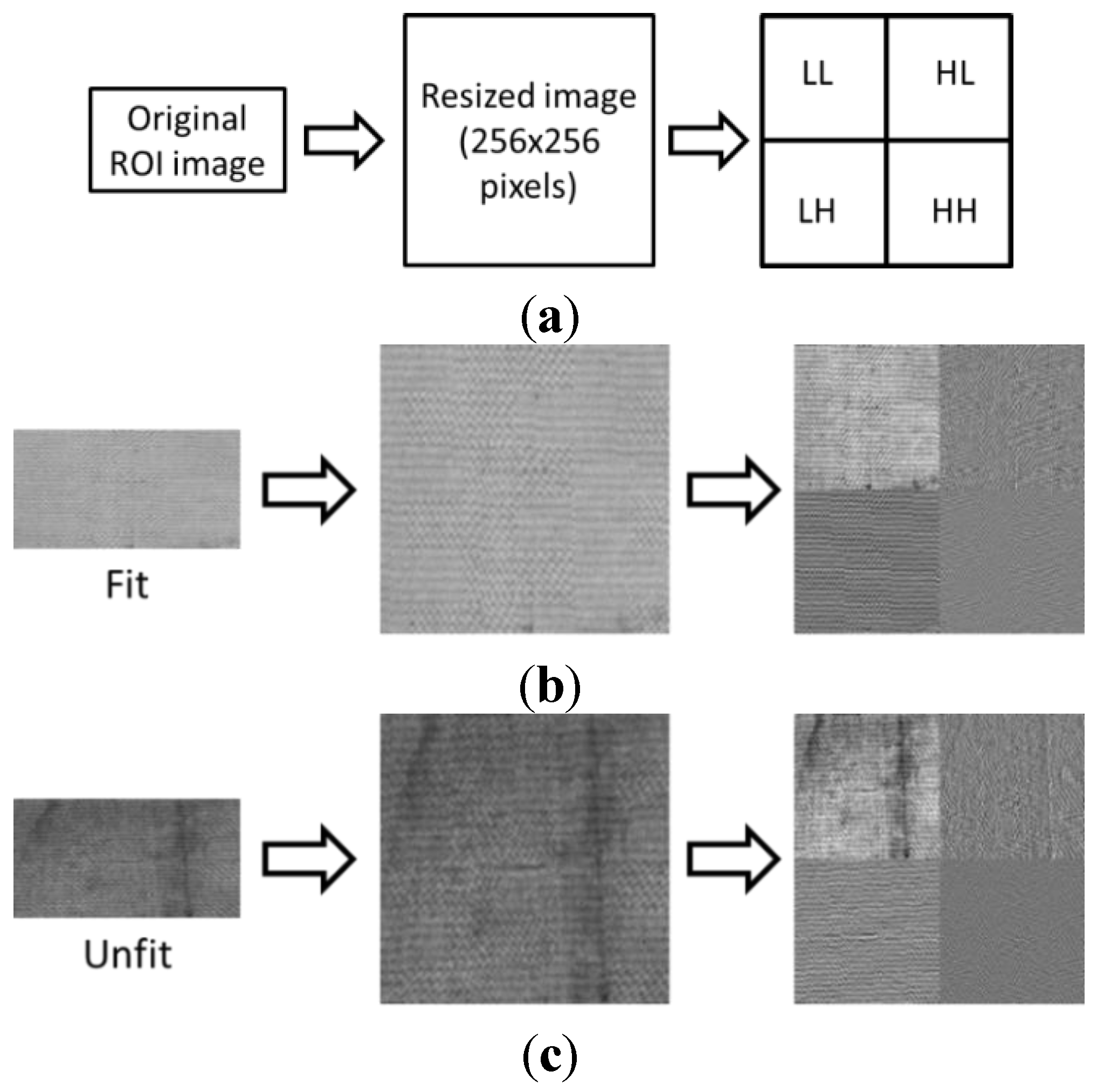
2.2. ROI Cropping and Feature Extraction


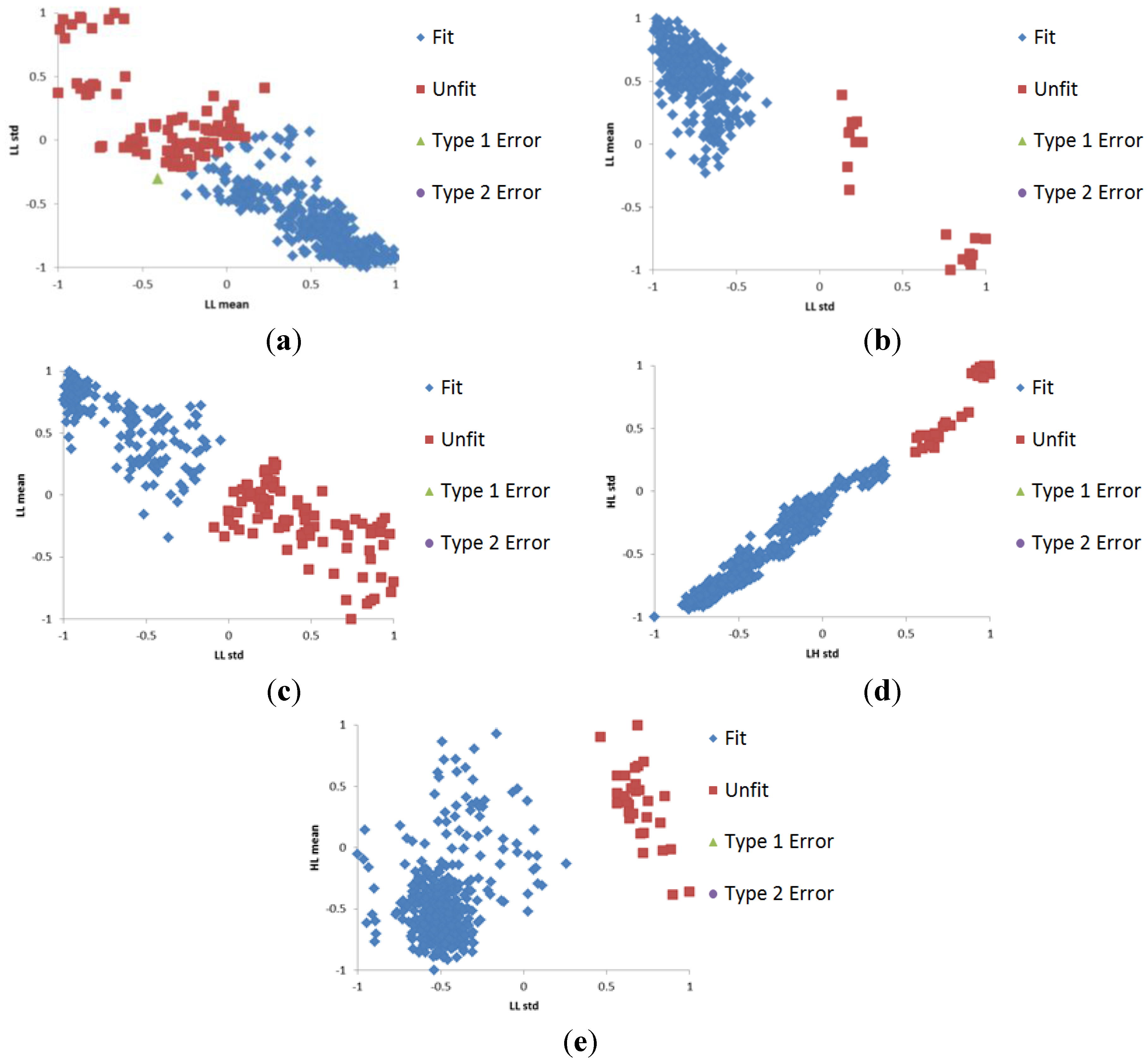
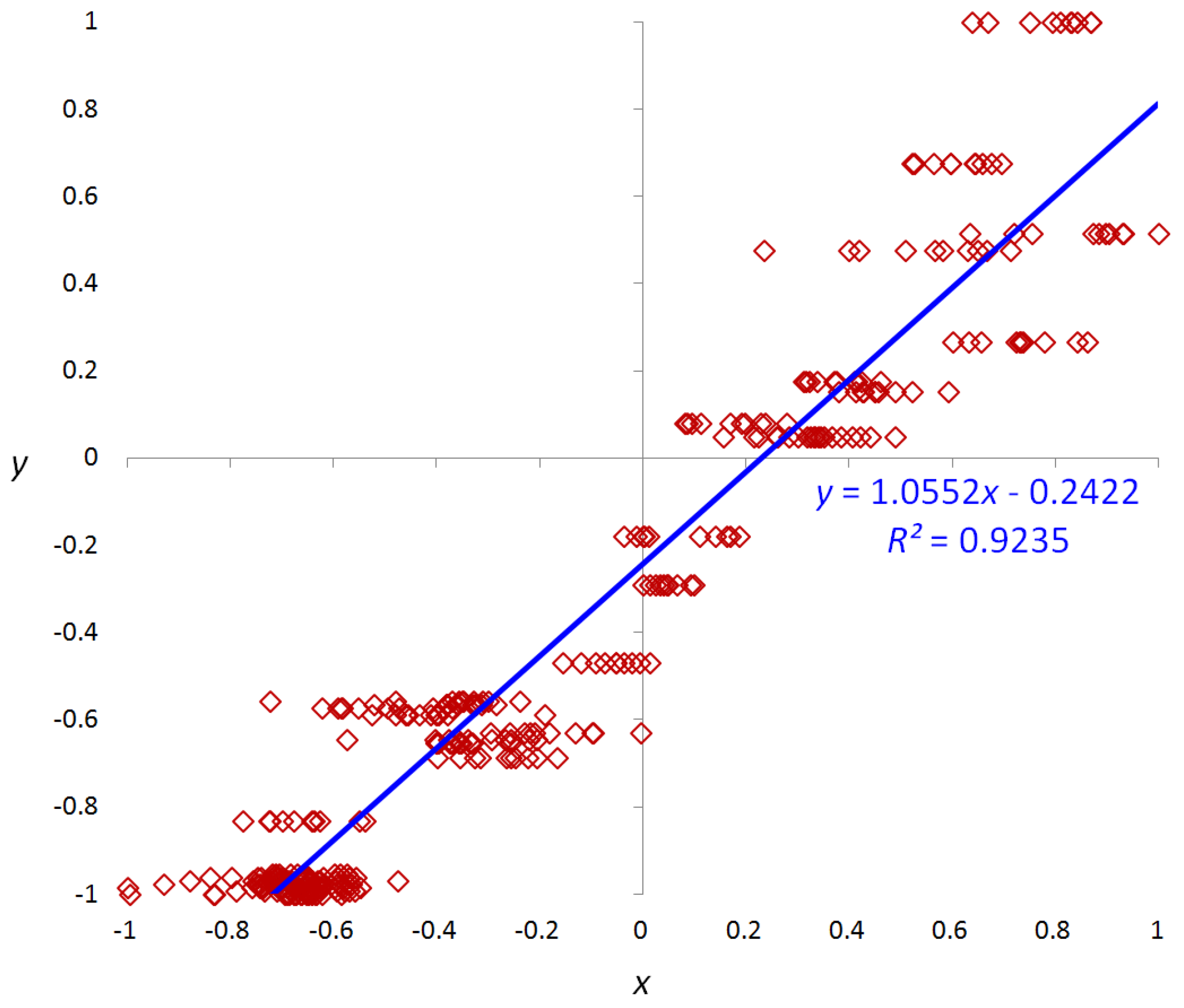
2.3. Selection of Optimal Features Using Regression Analysis
2.4. SVM Training and Testing
3. Experimental Results
| Denominations | A Direction | B Direction | C Direction | D Direction |
|---|---|---|---|---|
| 10 Rupee | 1040 | 1020 | 1020 | 1020 |
| 20 Rupee | 680 | 670 | 710 | 710 |
| 50 Rupee | 620 | 620 | 650 | 650 |
| 100 Rupee | 1540 | 1550 | 1520 | 1530 |
| 500 Rupee | 930 | 910 | 950 | 960 |
| Denom. | Dir. | Haar DWT | Daubechies DWT | ||||||
|---|---|---|---|---|---|---|---|---|---|
| Train 1—Test 2 | Train 2—Test 1 | Train 1—Test 2 | Train 2—Test 1 | ||||||
| Selected Features | R2 | Selected Features | R2 | Selected Features | R2 | Selected Features | R2 | ||
| 10 Rupee | A | LL mean | 0.6909 | LL mean | 0.8266 | LL mean | 0.6833 | LL mean | 0.8327 |
| LL std | 0.6437 | LL std | 0.7720 | LL std | 0.6365 | LL std | 0.7792 | ||
| B | LL mean | 0.6654 | LL mean | 0.8443 | LL mean | 0.6812 | LL mean | 0.8284 | |
| LL std | 0.6099 | LL std | 0.7455 | LL std | 0.6109 | LL std | 0.7477 | ||
| C | LH std | 0.9026 | LH std | 0.9296 | LH std | 0.8888 | LH std | 0.9197 | |
| LL mean | 0.8055 | HH std | 0.8691 | LL mean | 0.8176 | HL std | 0.8692 | ||
| D | LH std | 0.9052 | LH std | 0.9274 | LH std | 0.8845 | LH std | 0.9164 | |
| LL mean | 0.8300 | HH std | 0.8628 | LL mean | 0.8394 | HL std | 0.8587 | ||
| 20 Rupee | A | LL std | 0.7222 | LL std | 0.8243 | LL std | 0.7244 | LL std | 0.8238 |
| LL mean | 0.5351 | LL mean | 0.6733 | LL mean | 0.5682 | LL mean | 0.6864 | ||
| B | LL std | 0.7000 | LL std | 0.8075 | LL std | 0.6917 | LL std | 0.8239 | |
| LL mean | 0.5791 | LL mean | 0.6760 | LL mean | 0.5799 | LL mean | 0.6746 | ||
| C | LH std | 0.8287 | HL std | 0.7775 | LH std | 0.8034 | HL std | 0.7834 | |
| HL std | 0.7781 | LH std | 0.7412 | HL std | 0.7783 | LH std | 0.7439 | ||
| D | LH std | 0.8514 | LH std | 0.7314 | LH std | 0.8282 | LH std | 0.7526 | |
| HL std | 0.7964 | LL mean | 0.7096 | HL std | 0.7962 | LL mean | 0.7105 | ||
| 50 Rupee | A | LL std | 0.9018 | LL std | 0.9249 | LL std | 0.9043 | LL std | 0.9224 |
| LH std | 0.8949 | LL mean | 0.8764 | LL mean | 0.8526 | LL mean | 0.8887 | ||
| B | LL std | 0.8934 | LL std | 0.9315 | LL std | 0.8960 | LL std | 0.9274 | |
| LH std | 0.8778 | LL mean | 0.8762 | LL mean | 0.8557 | LL mean | 0.8817 | ||
| C | LH std | 0.9611 | LH std | 0.9390 | LH std | 0.9511 | LH std | 0.9235 | |
| LL mean | 0.9558 | HL std | 0.9144 | LL mean | 0.9471 | LL mean | 0.9087 | ||
| D | LH std | 0.9627 | LH std | 0.9450 | LH std | 0.9518 | LL mean | 0.9414 | |
| HL std | 0.9489 | LL mean | 0.9439 | LL mean | 0.9418 | LH std | 0.9374 | ||
| 100 Rupee | A | LH std | 0.8213 | LH std | 0.8307 | LH std | 0.7635 | LL std | 0.8234 |
| LL mean | 0.7222 | LL std | 0.8146 | LL mean | 0.7210 | LH std | 0.7917 | ||
| B | LH std | 0.8170 | LH std | 0.8249 | LL mean | 0.7160 | LL std | 0.8313 | |
| LL mean | 0.7395 | LL mean | 0.8062 | LL std | 0.7141 | LL mean | 0.8007 | ||
| C | LH std | 0.8599 | LH std | 0.8817 | LH std | 0.8276 | HL std | 0.8723 | |
| HL std | 0.8171 | HL std | 0.8638 | HL std | 0.7986 | LH std | 0.8694 | ||
| D | LH std | 0.8502 | LH std | 0.9030 | LH std | 0.8112 | LH std | 0.8476 | |
| HL std | 0.8073 | HL std | 0.8858 | LL mean | 0.7883 | HL std | 0.8448 | ||
| 500 Rupee | A | LL std | 0.6582 | LL std | 0.5521 | LL std | 0.6448 | LL std | 0.5581 |
| HL mean | 0.4041 | HL mean | 0.3839 | HL mean | 0.3582 | LL mean | 0.3580 | ||
| B | LL std | 0.4907 | LL std | 0.5184 | LL std | 0.5108 | LL std | 0.5510 | |
| HH std | 0.2833 | LL mean | 0.3015 | HL std | 0.2627 | LL mean | 0.3174 | ||
| C | LH std | 0.9314 | LH std | 0.8388 | LH std | 0.9105 | LH std | 0.7695 | |
| HL std | 0.9309 | HL std | 0.7307 | HL std | 0.8899 | LL mean | 0.6551 | ||
| D | HL std | 0.9291 | LH std | 0.8523 | LH std | 0.9270 | LH std | 0.8016 | |
| LH std | 0.9203 | HL std | 0.7639 | LL mean | 0.8959 | LL mean | 0.6472 | ||

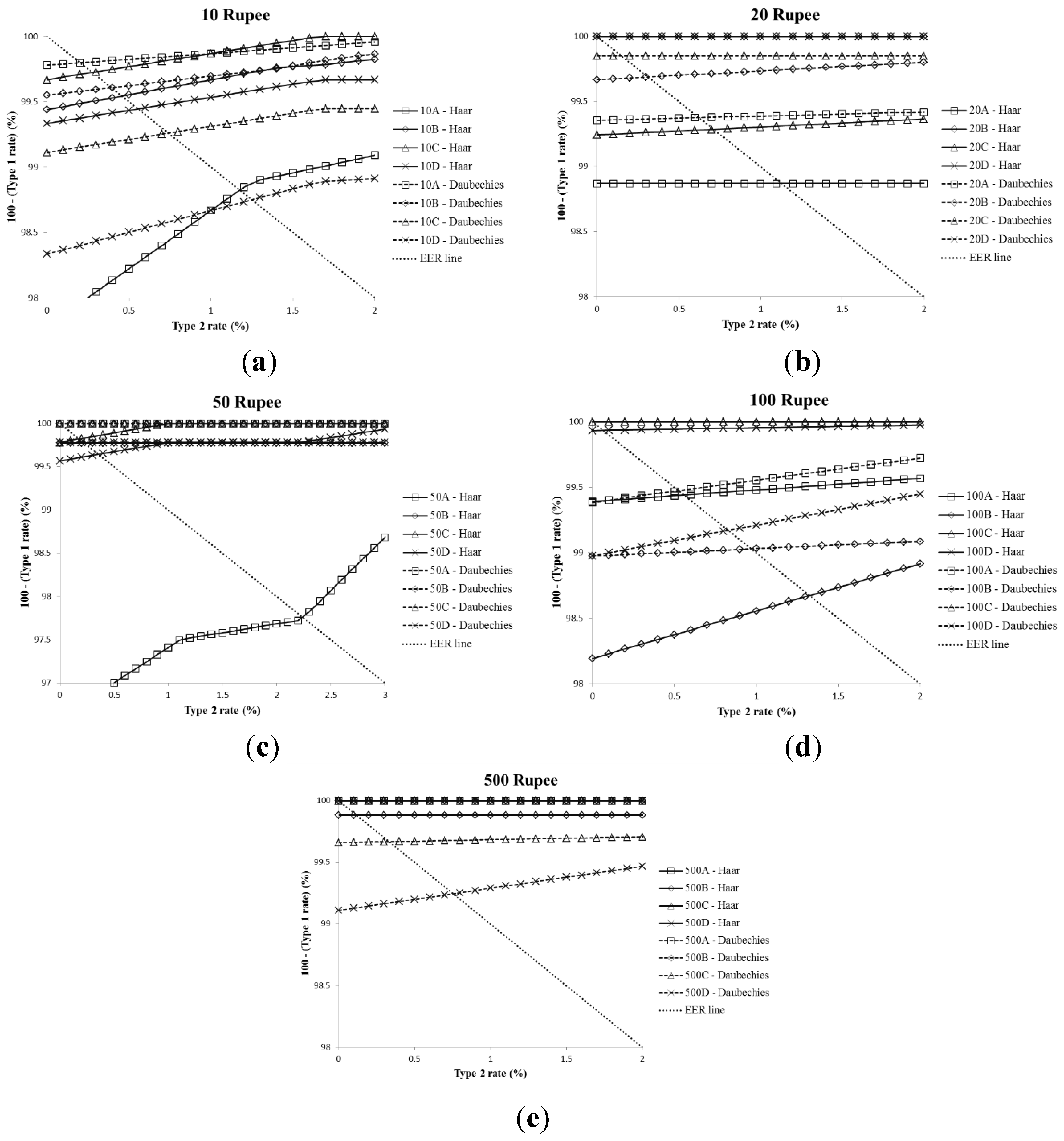
| Denom. | Dir. | SVM Kernel | Train 1—Test 2 | Train 2—Test 1 | Average EER | ||||
|---|---|---|---|---|---|---|---|---|---|
| Type 1 Error | Type 2 Error | EER | Type 1 Error | Type 2 Error | EER | ||||
| 10 Rupee | A | linear | 4.8889 | 0.0000 | 1.8841 | 0.0000 | 0.0000 | 0.0000 | 1.1764 |
| B | sigmoid | 2.7273 | 0.0000 | 0.3448 | 0.0000 | 3.3333 | 0.5882 | 0.4575 | |
| C | RBF | 2.0000 | 0.0000 | 0.4762 | 0.0000 | 1.6667 | 0.0000 | 0.2779 | |
| D | RBF | 0.6667 | 3.3333 | 0.9524 | 0.0000 | 1.6667 | 0.0000 | 0.5555 | |
| 20 Rupee | A | RBF | 0.0000 | 0.0000 | 0.0000 | 1.2903 | 40.0000 | 2.2581 | 1.1290 |
| B | RBF | 0.0000 | 5.0000 | 0.0000 | 0.0000 | 0.0000 | 0.0000 | 0.0000 | |
| C | RBF | 0.0000 | 0.0000 | 0.0000 | 0.0000 | 35.0000 | 1.3514 | 0.7142 | |
| D | linear | 0.0000 | 0.0000 | 0.0000 | 0.0000 | 0.0000 | 0.0000 | 0.0000 | |
| 50 Rupee | A | RBF | 0.4545 | 16.6667 | 2.8947 | 2.0833 | 0.0000 | 0.0000 | 2.2385 |
| B | linear | 0.4545 | 0.0000 | 0.4545 | 3.7500 | 0.0000 | 0.0000 | 0.2275 | |
| C | linear | 0.4348 | 1.0000 | 0.3030 | 0.0000 | 0.0000 | 0.0000 | 0.1786 | |
| D | RBF | 0.4348 | 0.0000 | 0.3030 | 2.1739 | 0.0000 | 0.4348 | 0.3573 | |
| 100 Rupee | A | linear | 0.0000 | 12.0000 | 0.9524 | 0.0000 | 12.0000 | 0.1333 | 0.5605 |
| B | linear | 0.0000 | 4.0000 | 0.0000 | 0.8333 | 7.5000 | 2.0968 | 1.3266 | |
| C | linear | 0.0000 | 0.0000 | 0.0000 | 0.0000 | 0.0000 | 0.0000 | 0.0000 | |
| D | linear | 0.2703 | 0.0000 | 0.0000 | 0.0000 | 23.3333 | 0.1316 | 0.0671 | |
| 500 Rupee | A | poly | 0.4651 | 0.0000 | 0.0000 | 0.0000 | 0.0000 | 0.0000 | 0.0000 |
| B | sigmoid | 0.0000 | 50.0000 | 0.2381 | 1.1111 | 0.0000 | 0.0000 | 0.1190 | |
| C | sigmoid | 2.9545 | 0.0000 | 0.0000 | 0.0000 | 0.0000 | 0.0000 | 0.0000 | |
| D | sigmoid | 3.1111 | 0.0000 | 0.0000 | 0.0000 | 3.3333 | 0.0000 | 0.0000 | |
| Average EER | 0.4693 | ||||||||
| Denom. | Dir. | SVM Kernel | Train 1–Test 2 | Train 2–Test 1 | Average EER | ||||
|---|---|---|---|---|---|---|---|---|---|
| Type 1 Error | Type 2 Error | EER | Type 1 Error | Type 2 Error | EER | ||||
| 10 Rupee | A | linear | 4.2222 | 0.0000 | 0.3774 | 0.0000 | 1.6667 | 0.0000 | 0.2039 |
| B | linear | 1.1364 | 0.0000 | 0.5882 | 0.0000 | 6.6667 | 0.1961 | 0.3944 | |
| C | RBF | 2.6667 | 0.0000 | 1.1765 | 0.0000 | 1.6667 | 0.3509 | 0.7405 | |
| D | sigmoid | 0.2222 | 8.3333 | 2.1569 | 0.6667 | 0.0000 | 0.0000 | 1.2499 | |
| 20 Rupee | A | sigmoid | 0.0000 | 0.0000 | 0.0000 | 1.2903 | 0.0000 | 1.2121 | 0.6249 |
| B | sigmoid | 0.0000 | 0.0000 | 0.0000 | 0.0000 | 30.0000 | 0.5882 | 0.3126 | |
| C | sigmoid | 0.0000 | 0.0000 | 0.0000 | 0.3030 | 20.0000 | 0.3030 | 0.1515 | |
| D | linear | 0.0000 | 0.0000 | 0.0000 | 0.0000 | 0.0000 | 0.0000 | 0.0000 | |
| 50 Rupee | A | linear | 0.0000 | 0.0000 | 0.0000 | 0.8333 | 0.0000 | 0.0000 | 0.0000 |
| B | linear | 0.4545 | 0.0000 | 0.0000 | 0.4167 | 0.0000 | 0.0000 | 0.0000 | |
| C | linear | 0.0000 | 3.0000 | 0.0000 | 3.0435 | 0.0000 | 0.0000 | 0.0000 | |
| D | sigmoid | 0.0000 | 0.0000 | 0.0000 | 1.3043 | 0.0000 | 0.4348 | 0.2175 | |
| 100 Rupee | A | linear | 0.0000 | 8.0000 | 0.5051 | 0.0000 | 8.0000 | 0.5556 | 0.5269 |
| B | RBF | 0.4054 | 4.0000 | 1.2162 | 0.2778 | 5.0000 | 0.7500 | 0.9707 | |
| C | linear | 0.0000 | 0.0000 | 0.0000 | 0.0000 | 16.6667 | 0.0000 | 0.0000 | |
| D | poly | 0.4054 | 0.0000 | 0.3822 | 0.0000 | 26.6667 | 1.1650 | 0.8290 | |
| 500 Rupee | A | linear | 0.4651 | 0.0000 | 0.0000 | 0.0000 | 3.3333 | 0.0000 | 0.0000 |
| B | linear | 0.0000 | 25.0000 | 0.0000 | 0.0000 | 0.0000 | 0.0000 | 0.0000 | |
| C | linear | 2.9545 | 0.0000 | 0.6522 | 0.0000 | 13.3333 | 0.0000 | 0.3334 | |
| D | RBF | 2.6667 | 0.0000 | 1.3115 | 0.0000 | 0.0000 | 0.0000 | 0.7548 | |
| Average EER | 0.3655 | ||||||||
| Correct Classification | Type 1 Error Case | Type 2 Error Case | ||
|---|---|---|---|---|
| Fit case | Unfit case | |||
| Cropped ROI |  |  |  | 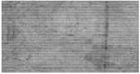 |
| Image by Haar DWT | 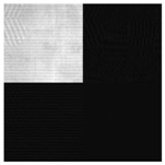 |  | 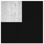 | 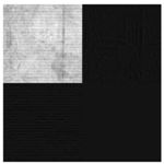 |

| Denomination | Direction | Haar DWT | Daubechies DWT | Previous Method [7] |
|---|---|---|---|---|
| 10 Rupee | A | 1.1764 | 0.2039 | 6.9036 |
| B | 0.4575 | 0.3944 | 16.2962 | |
| C | 0.2779 | 0.7405 | 6.2792 | |
| D | 0.5555 | 1.2499 | 16.5487 | |
| 20 Rupee | A | 1.1290 | 0.6249 | 25.0000 |
| B | 0.0000 | 0.3126 | 25.3456 | |
| C | 0.7142 | 0.1515 | 26.7717 | |
| D | 0.0000 | 0.0000 | 28.7490 | |
| 50 Rupee | A | 2.2385 | 0.0000 | 5.2397 |
| B | 0.2275 | 0.0000 | 16.0191 | |
| C | 0.1786 | 0.0000 | 2.8302 | |
| D | 0.3573 | 0.2175 | 0.0000 | |
| 100 Rupee | A | 0.5605 | 0.5269 | 1.2179 |
| B | 1.3266 | 0.9707 | 2.1053 | |
| C | 0.0000 | 0.0000 | 0.6868 | |
| D | 0.0671 | 0.8290 | 1.3765 | |
| 500 Rupee | A | 0.0000 | 0.0000 | 25.0000 |
| B | 0.1190 | 0.0000 | 25.0000 | |
| C | 0.0000 | 0.3334 | 0.0000 | |
| D | 0.0000 | 0.7548 | 0.0000 | |
| Average EER | 0.4693 | 0.3655 | 11.5685 | |
4. Conclusions
Acknowledgments
Author Contributions
Conflicts of Interest
References
- Geusebroek, J.M.; Markus, P.; Balke, P. Learning Banknote Fitness for Sorting. In Proceedings of the International Conference on Pattern Analysis and Intelligent Robotics, Putrajaya, Malaysia, 28–29 June 2011; pp. 41–46.
- De Heij, H. Durable Banknotes: An Overview. In Presented at the BPC/Paper Committee to the BPC/General Meeting, Prague, Czech, 27–30 May 2002; pp. 1–12.
- Balke, P. From Fit to Unfit: How Banknotes Become Soiled. In Proceedings of the Fourth International Scientific and Practical Conference on Security Printing Watermark Conference, Rostov-on-Don, Russia, 21–23 June 2011.
- Buitelaar, T. The Colour of Soil. In Presented at the DNB Cash Seminar, Amsterdam, The Netherlands, 28–29 February 2008.
- Balke, P.; Geusebroek, J.M.; Markus, P. BRAIN2—Machine Learning to Measure Banknote Fitness. In Proceedings of the Optical Document Security Conference, San Francisco, CA, USA, 18–20 January 2012.
- Aoba, M.; Kikuchi, T.; Takefuji, Y. Euro banknote recognition system using a three-layered perceptron and RBF networks. IPSJ Trans. Math. Model. Appl. 2003, 44, 99–109. [Google Scholar]
- He, K.; Peng, S.; Li, S. A Classification Method for the Dirty Factor of Banknotes Based on Neural Network with Sine Basis Functions. In Proceedings of the International Conference on Intelligent Computation Technology and Automation, Hunan, China, 20–22 October 2008; pp. 159–162.
- Rahman, M.M.; Poon, B.; Amin, M.A.; Yan, H. Recognizing Bangladeshi currency for visually impaired. Commun. Comput. Inform. Sci. 2014, 481, 129–135. [Google Scholar]
- Chetan, B.V.; Vijaya, P.A. A robust side invariant technique of Indian paper currency recognition. Int. J. Eng. Res. Technol. 2012, 1, 1–7. [Google Scholar]
- Verma, K.; Singh, B.K.; Agarwal, A. Indian Currency Recognition Based on Texture Analysis. In Proceedings of the Nirma University International Conference on Engineering, Ahmedabad, Gujarat, India, 8–10 December 2011; pp. 1–5.
- Sharma, B.; Kaur, A.; Vipan, D. Recognition of Indian paper currency based on LBP. Int. J. Comput. Appl. 2012, 59, 24–27. [Google Scholar] [CrossRef]
- Pathrabe, T.; Karmore, S. A novel approach of embedded system for Indian paper currency recognition. Int. J. Comput. Trends Technol. 2011, 1, 152–156. [Google Scholar]
- Sanjana, M.; Diwakar, M.; Sharma, A. An automated recognition of fake or destroyed Indian currency notes in machine vision. Int. J. Comput. Sci. Manag. Stud. 2012, 12, 53–60. [Google Scholar]
- Choi, E.; Lee, J.; Yoon, J. Feature Extraction for Bank Note Classification Using Wavelet Transform. In Proceedings of the 18th International Conference on Pattern Recognition, Hong Kong, China, 20–24 August 2006; pp. 934–937.
- Ahangaryan, F.P.; Mohammadpour, T.; Kianisarkaleh, A. Persian Banknote Recognition Using Wavelet and Neural Network. In Proceedings of the International Conference on Computer Science and Electronics Engineering, Hangzhou, China, 23–25 March 2012; pp. 679–684.
- Gonzalez, R.C.; Woods, R.E. Digital Image Processing, 3rd ed.; Prentice Hall: Upper Saddle River, NJ, USA, 2010. [Google Scholar]
- Nguyen, D.T.; Park, Y.H.; Shin, K.Y.; Kwon, S.Y.; Lee, H.C.; Park, K.R. Fake finger-vein image detection based on fourier and wavelet transforms. Digit. Signal. Process. 2013, 23, 1401–1413. [Google Scholar] [CrossRef]
- Simple Linear Regression. Available online: http://en.wikipedia.org/wiki/Simple_linear_regression (accessed on 17 May 2015).
- Coefficient of Determination. Available online: http://en.wikipedia.org/wiki/Coefficient_of_determination (accessed on 17 May 2015).
- Densitometer. Available online: http://www.xrite.com/documents/literature/gmb/en/100_d19_en.pdf (accessed on 17 May 2015).
- State Bank of India, Request for Proposal. Available online: http://www.sbi.co.in/portal/web/home/tenders-awarded (accessed on 26 July 2015).
- Hsu, C.W.; Chang, C.C.; Lin, C.J. A Practical Guide to Support. Vector Classification; Technical Report for National Taiwan University: Taipei, Taiwan, 2003. [Google Scholar]
- Chang, C.-C.; Lin, C.-J. LIBSVM: A library for support vector machines. ACM Trans. Intell. Syst. Technol. 2011, 2, 27. [Google Scholar] [CrossRef]
- Hagan, M.T.; Demuth, H.B.; Beale, M.H. Neural Network Design; PWS Publishing Co.: Boston, MA, USA, 1995. [Google Scholar]
© 2015 by the authors; licensee MDPI, Basel, Switzerland. This article is an open access article distributed under the terms and conditions of the Creative Commons Attribution license (http://creativecommons.org/licenses/by/4.0/).
Share and Cite
Pham, T.D.; Park, Y.H.; Kwon, S.Y.; Nguyen, D.T.; Vokhidov, H.; Park, K.R.; Jeong, D.S.; Yoon, S. Recognizing Banknote Fitness with a Visible Light One Dimensional Line Image Sensor. Sensors 2015, 15, 21016-21032. https://doi.org/10.3390/s150921016
Pham TD, Park YH, Kwon SY, Nguyen DT, Vokhidov H, Park KR, Jeong DS, Yoon S. Recognizing Banknote Fitness with a Visible Light One Dimensional Line Image Sensor. Sensors. 2015; 15(9):21016-21032. https://doi.org/10.3390/s150921016
Chicago/Turabian StylePham, Tuyen Danh, Young Ho Park, Seung Yong Kwon, Dat Tien Nguyen, Husan Vokhidov, Kang Ryoung Park, Dae Sik Jeong, and Sungsoo Yoon. 2015. "Recognizing Banknote Fitness with a Visible Light One Dimensional Line Image Sensor" Sensors 15, no. 9: 21016-21032. https://doi.org/10.3390/s150921016
APA StylePham, T. D., Park, Y. H., Kwon, S. Y., Nguyen, D. T., Vokhidov, H., Park, K. R., Jeong, D. S., & Yoon, S. (2015). Recognizing Banknote Fitness with a Visible Light One Dimensional Line Image Sensor. Sensors, 15(9), 21016-21032. https://doi.org/10.3390/s150921016