
Hyperspectral Analysis of Soil Total Nitrogen in Subsided Land Using the Local Correlation Maximization-Complementary Superiority (LCMCS) Method

Abstract
:1. Introduction

| Research Field | Sensors | Factor Monitored | Application | Reference |
|---|---|---|---|---|
| Water | Ocean Optics USB4000 | Chlorophyll a | Estimation of chlorophyll-a in turbid inland waters | [33] |
| ASD | Fucoxanthin, zeaxanthin, chlorophyll a and chlorophyll b | Quantification of diatom biomass in Microphytobenthic (MPB) biofilms (non-destructively) | [34] | |
| ASD, ATM-2 | Grain size | Characterization and management of the beach environment | [35] | |
| Plants | Airborne HyMap | Foliar nitrogen | prediction of sagebrush canopy nitrogen from an airborne platform | [36] |
| Perkin Elmer Lamdba 19 | Leaf pigment, Chlorophyll, Carotenoid, Nitrogen, Carbon | Spectroscopy of plant biochemistry | [37] | |
| ASD | Leaf chlorophyll | Retrieval of spatially-continuous leaf chlorophyll content | [38] | |
| ASD | Major plant species | Classification of Hyperspectral images | [39] | |
| ASD | Fusarium circinatum Stress | Early detection of Fusarium circinatum-induced stress in Pinus radiata seedlings. | [40] | |
| ProSpecTIR-VS, ASD | Plant stress | The Plant Stress Detection Index (PSDI) used as plant stress indicator | [41] | |
| ASD | Mangrove leaves | Mangrove classification | [42] | |
| ASD | Water stress | Prediction of Grain and biomass yield of wheat based on water stress indices | [43] | |
| ASD, Ocean Optics (QE65000, Jaz) | pH | Determination of pH in Sala mango | [44] | |
| ASD | Zn content | Monitoring Zn nutrient levels under field conditions | [45] | |
| ASD | Leaf chlorophyll | Validation of satellites’ vegetation products | [46] | |
| Soils | ASD | Soil nitrogen, carbon, carbonate, and organic matter | Assessing nitrogen, carbon, carbonate and organic matter for upper soil horizons (non-destructively). | [6] |
| ALPHA FT-IR | Soil carbon | Soil carbon validation at large scale | [13] | |
| HySpex VNIR-1600 | Soil carbon, nitrogen, aluminum, iron and manganese | Improvement of soil classification, assessment of elemental budgets and balances and understanding of soil forming processes and mechanisms. | [14] | |
| ASD | Soil bulk density, moisture content, clay, silt, and sand | Estimating the physical properties of paddy soil | [47] |
2. Materials and Methods

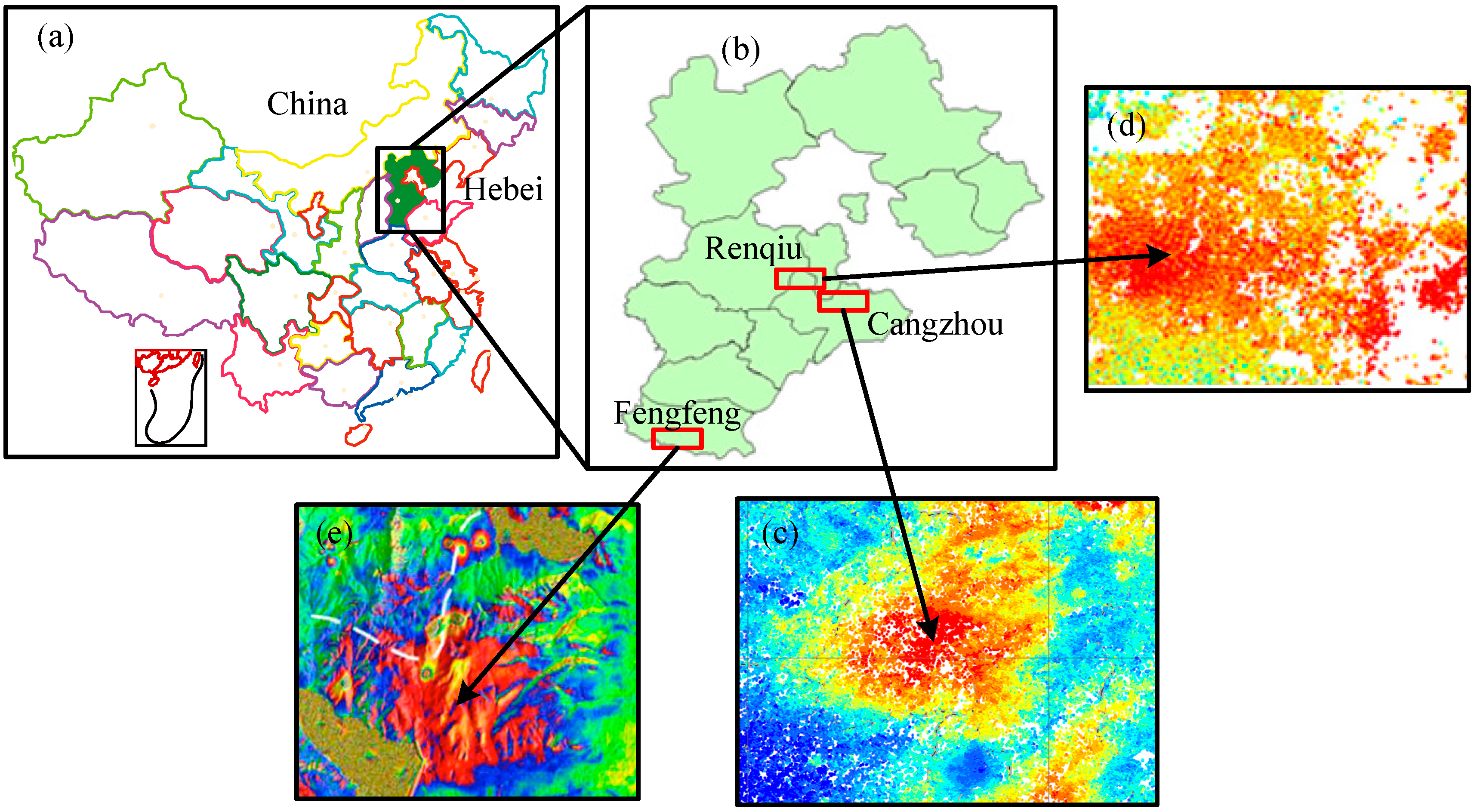
2.1. Experiment
2.1.1. Sample Preparation
| City | Soil Types |
|---|---|
| Changzhou | Fluvo-aquic soil, Salinized fluvo-aquic soil |
| Renqiu | Fluvo-aquic soil, Salinized fluvo-aquic soil |
| Fengfeng | Cinnamon soil |
2.1.2. Measurement and Data Processing
2.1.3. Spectral Transformations
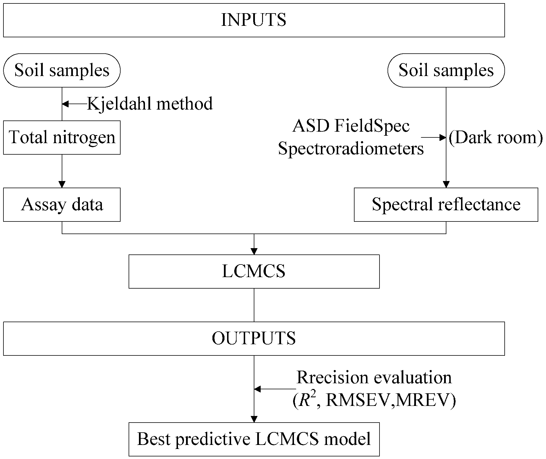
2.1.4. Retrieval Model
2.2. Methods
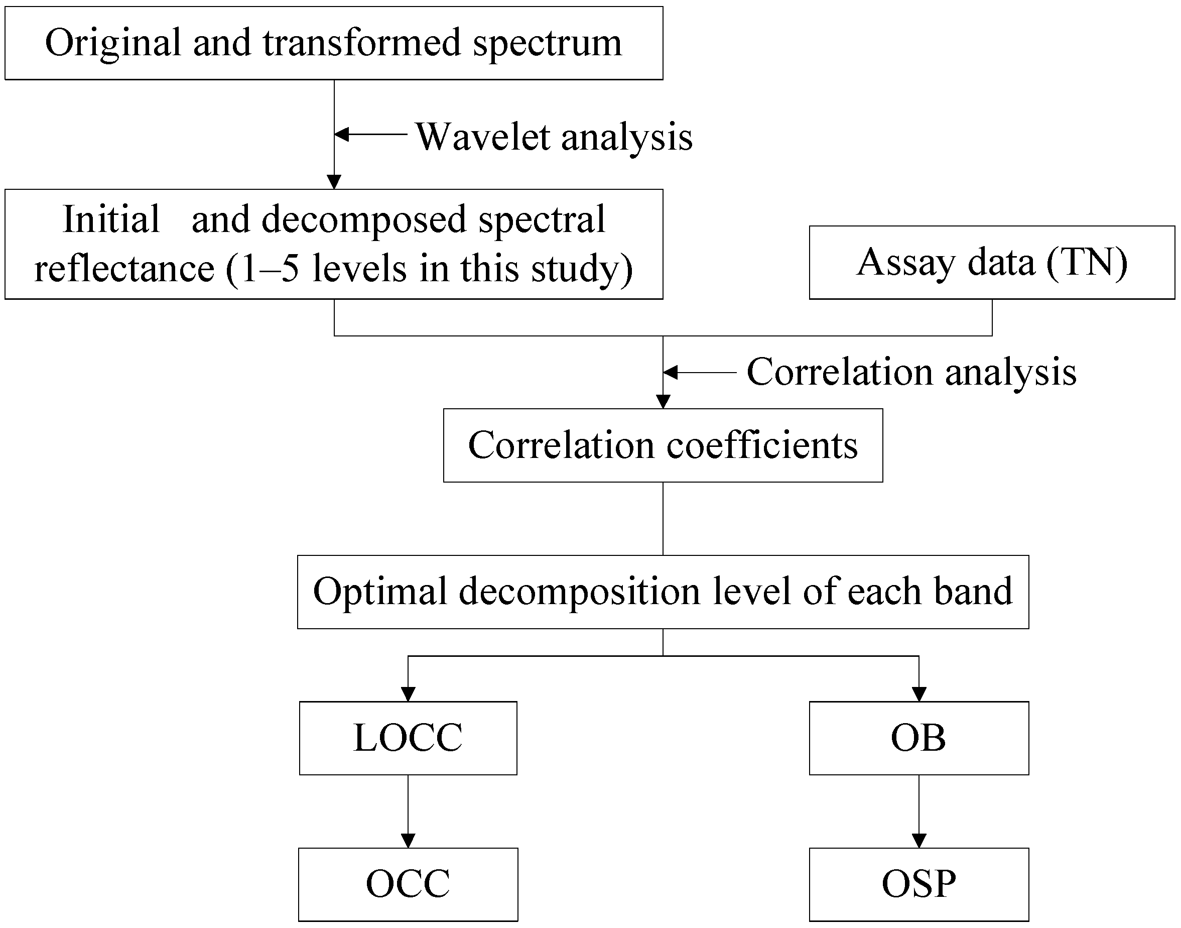
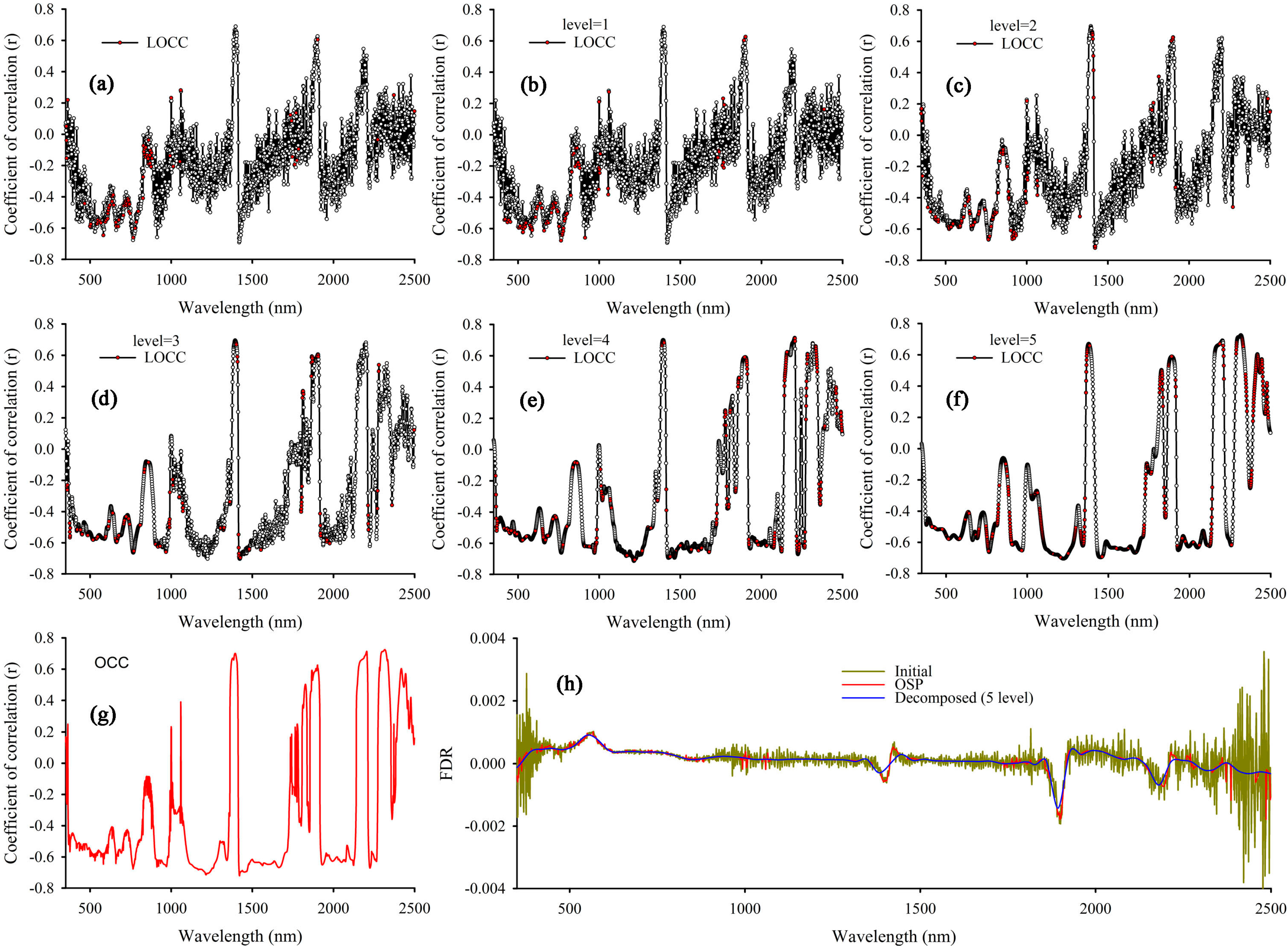
2.2.1. Local Correlation Maximization De-Noising Method (LCM)
- (1)
- Decomposing the original and transformed spectrum into five layers using a wavelet de-noising method that is based on the Sym8 matrix function.
- (2)
- Calculating the correlation coefficients for the measured TN content compared with both initial (including original and transformed spectrum, the same hereafter) and decomposed spectral reflectance (1–5 levels in this study), in the range of 350–2500 nm.
- (3)
- Finding the optimal decomposition level of each band, which has the maximum correlation coefficient among initial and decomposed spectra (1–5 levels) at each wavelength; then, the corresponding correlation coefficient and decomposed band are taken as the local optimal correlation coefficient (LOCC) and optimal band (OB). After all the LOCCs and OBs are acquired, the overall LOCC and OB are used to determine the optimal correlative curve (OCC) and the optimal spectra (OSP), respectively. Finally, the OSP and OCC of original and transformed spectra are obtained, Figure 3 shows the overall approach.

2.2.2. Partial Least Square Regression (PLS Regression) Method
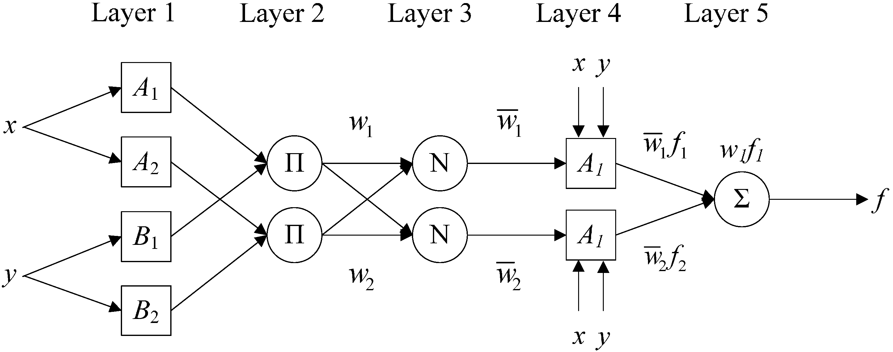
2.2.3. Adaptive Neuro-Fuzzy Inference System (ANFIS)

2.2.4. Local Correlation Maximization-Complementary Superiority (LCMCS)
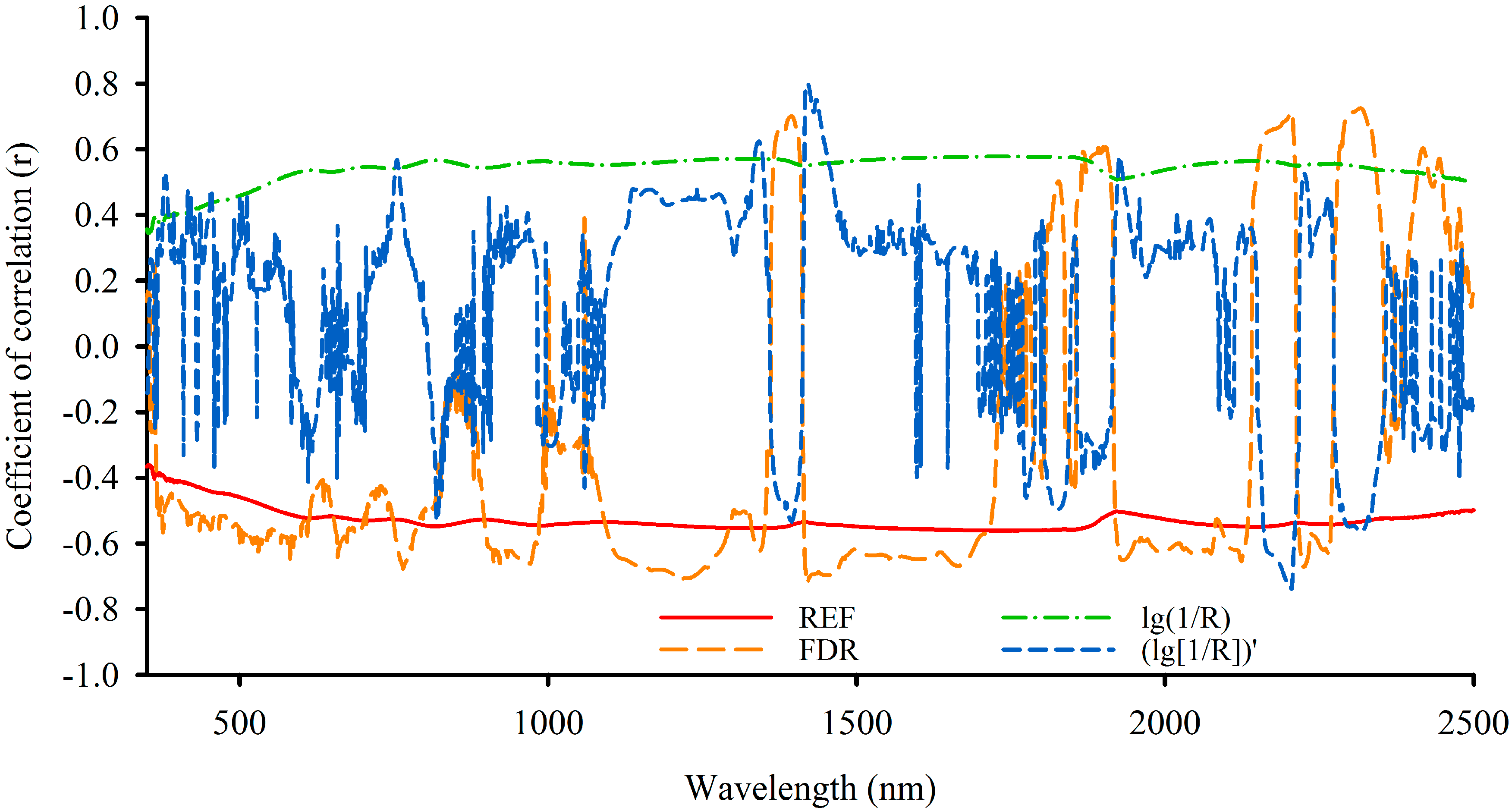
- (1)
- Spectral transforms. Spectral transforms help reduce the influence of noise; therefore, each REF is transformed into FDR, log(1/R) and (log[1/R])′.
- (2)
- LCM analysis. To maximize the use of TN response information and eliminate the interference of noisy data, OSP and OCC of the original and transformed spectrum are obtained by LCM de-noising method, which has significant correlativity with TN content.
- (3)
- Complementary superiority. OSP and measured TN values are used in PLS regression analysis, and several principal components (five principal components in this study) are acquired. These principal components and the measured TN contents are then used in ANFIS analysis, and the LCMCS models are established.
- (4)
- Model-verifying. Sample data are used for model calibration and verification. In this study, from the 280 samples in each treatment, 150 samples were used for model calibration and the remaining 130 samples were used for model verification. Then, the best model was selected as the final model using the LCMCS method.
2.2.5. Model Evaluation Standard
| Dataset | NS | EP | |
|---|---|---|---|
| Calibration | 150 | 55 C | R2, RMSEC, MREC |
| 50 R | |||
| 45 F | |||
| Validation | 130 | 45 C | R2, RMSEV, MREV |
| 45 R | |||
| 40 F | |||
3. Results and Discussion
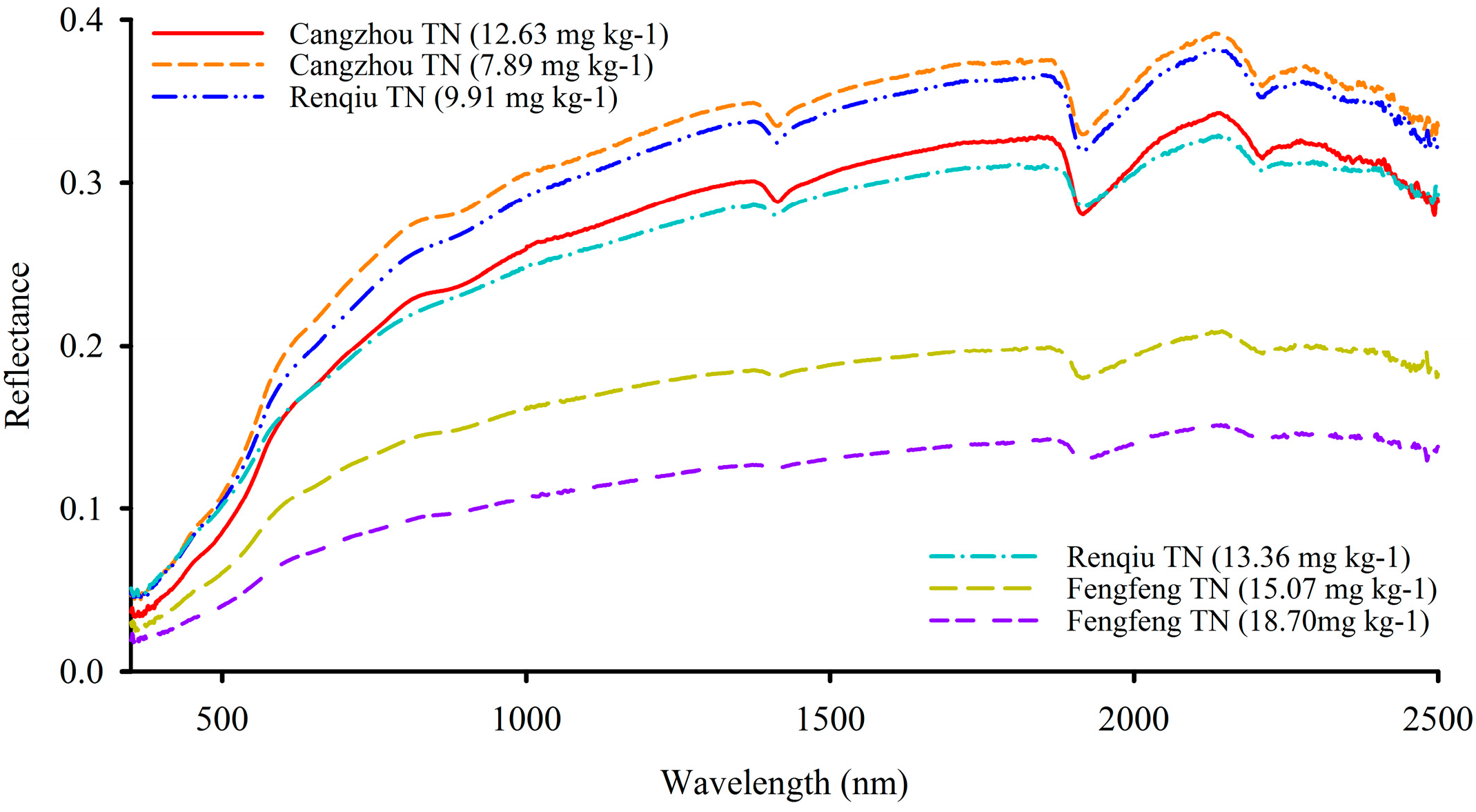
3.1. Interpretation of Soil Spectral Reflectance
3.2. OSP Acquisition
| TSP | MPCB (nm) | CC | MNCB (nm) | CC | AACC |
|---|---|---|---|---|---|
| FDR | 1397 | 0.669 | 766 | −0.672 | 0.253 |
| FDR (DL = 1) | 1397 | 0.689 | 1419 | −0.692 | 0.266 |
| FDR (DL = 2) | 1395 | 0.697 | 1421 | −0.721 | 0.331 |
| FDR (DL = 3) | 1394 | 0.695 | 1422 | −0.704 | 0.422 |
| FDR (DL = 4) | 2205 | 0.714 | 1214 | −0.715 | 0.482 |
| FDR (DL = 5) | 2316 | 0.725 | 1223 | −0.706 | 0.500 |
| TSP | CL | NB | MPCB (nm) | CC | MNCB (nm) | CC |
|---|---|---|---|---|---|---|
| FDR | ** | 2023 | 2316 | 0.725 | 1421 | −0.721 |
| >0.40 | 1759 | 2316 | 0.725 | 1421 | −0.721 | |
| >0.45 | 1654 | 2316 | 0.725 | 1421 | −0.721 | |
| >0.50 | 1510 | 2316 | 0.725 | 1421 | −0.721 | |
| >0.55 | 1291 | 2316 | 0.725 | 1421 | −0.721 | |
| >0.60 | 949 | 2316 | 0.725 | 1421 | −0.721 | |
| (log[1/R])′ | ** | 1655 | 1422 | 0.797 | 2205 | −0.739 |
| >0.40 | 566 | 1422 | 0.797 | 2205 | −0.739 | |
| >0.45 | 392 | 1422 | 0.797 | 2205 | −0.739 | |
| >0.50 | 210 | 1422 | 0.797 | 2205 | −0.739 | |
| >0.55 | 134 | 1422 | 0.797 | 2205 | −0.739 | |
| >0.60 | 92 | 1422 | 0.797 | 2205 | −0.739 |

3.3. Applicability of LCMCS Model
| TSP | CL | LVs | Calibration (n = 150) | Validation (n = 130) | ||||
|---|---|---|---|---|---|---|---|---|
| R2 | RMSEC | MREC | R2 | RMSEV | MREV | |||
| FDR | ** | 5 | 0.951 | 0.629 | 3.311 | 0.808 | 1.169 | 7.901 |
| >0.40 | 5 | 0.946 | 0.667 | 3.818 | 0.829 | 1.095 | 7.901 | |
| >0.45 | 5 | 0.923 | 0.793 | 4.909 | 0.834 | 1.076 | 6.969 | |
| >0.50 | 5 | 0.920 | 0.808 | 5.231 | 0.823 | 1.105 | 6.890 | |
| >0.55 | 5 | 0.927 | 0.767 | 4.781 | 0.831 | 1.080 | 7.051 | |
| >0.60 | 5 | 0.917 | 0.821 | 5.168 | 0.797 | 1.184 | 8.068 | |
| (log[1/R])′ | ** | 5 | 0.991 | 0.269 | 1.446 | 0.885 | 0.898 | 5.921 |
| >0.40 | 5 | 0.939 | 0.704 | 4.220 | 0.681 | 1.529 | 9.613 | |
| >0.45 | 5 | 0.910 | 0.854 | 5.009 | 0.817 | 1.123 | 7.602 | |
| >0.50 | 5 | 0.953 | 0.616 | 3.615 | 0.785 | 1.240 | 8.178 | |
| >0.55 | 5 | 0.954 | 0.608 | 3.037 | 0.779 | 1.234 | 7.626 | |
| >0.60 | 5 | 0.957 | 0.588 | 2.968 | 0.776 | 1.255 | 7.815 | |
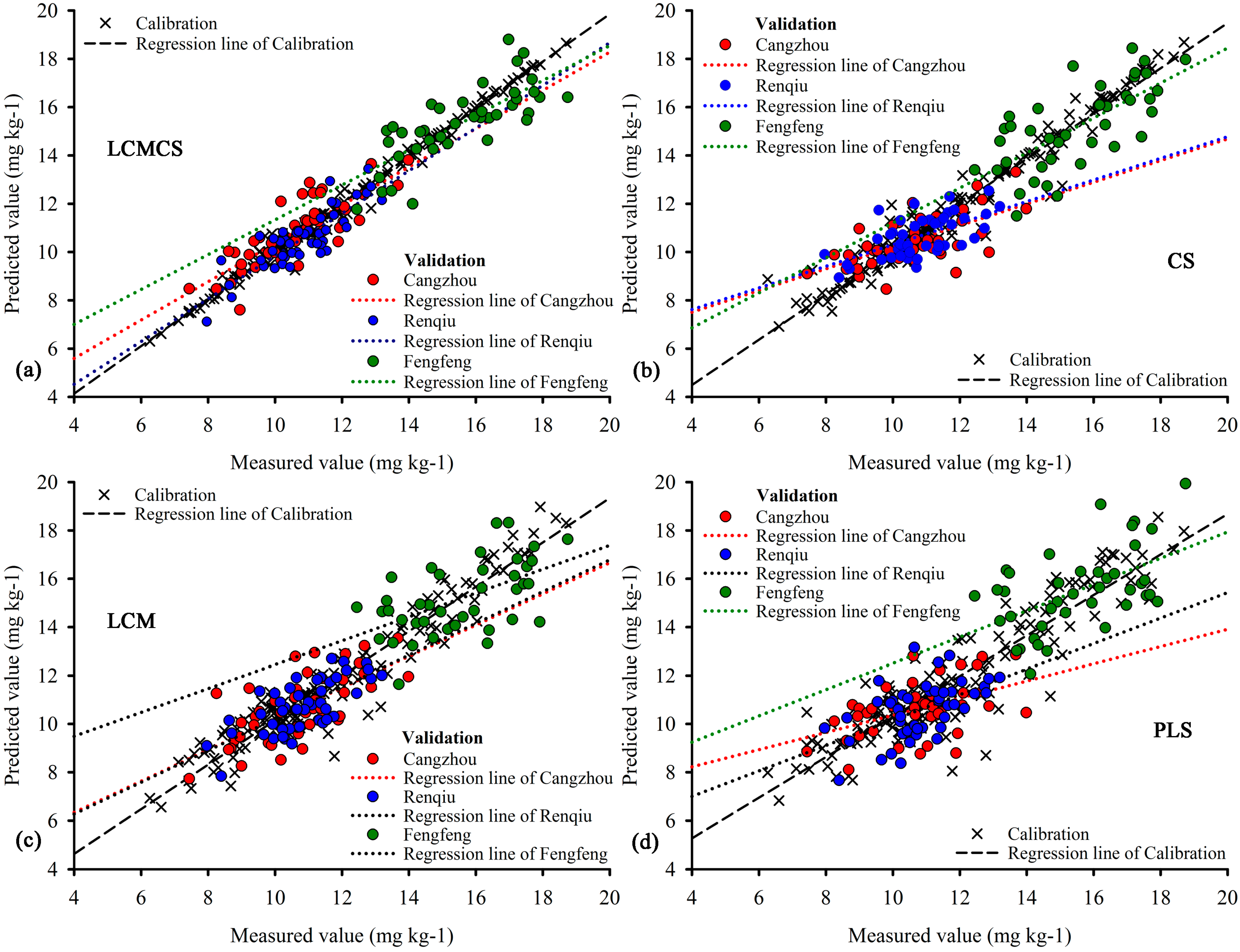
- (1)
- PLS regression method. In PLS regression models, decomposed FDR (5 level) and (log[1/R])′ (4 level), whose correlation coefficients reached to 0.725 and 0.797, respectively, were used in PLS analysis. Based on the 1293 selected effective bands of (log[1/R])′ (5 level), whose correlation coefficients were significant (p < 0.01), the optimal model of PLS method was obtained, which was selected as the final model of the PLS regression method.
- (2)
- Local correlation maximization method (LCM). Facing the second issue of how to reduce noise while retaining as much useful information as possible, OSP of FDR and (log[1/R])′ were used in PLS regression analysis. Based on the 1655 selected effective bands of (log[1/R])′ (OSP), whose correlation coefficients were significant (p < 0.01), the optimal model of the LCM method was obtained and selected as the final model of the LCM method.
- (3)
- Complementary superiority method (CS). The CS model, which had the advantages of PLS regression and ANFIS, was aimed at addressing the third issue. The same PLS regression models, decomposed FDR (5 level) and (log[1/R])′ (4 level) were used. Based on the 382 selected effective bands of (log[1/R])′ (4 level), whose correlation coefficients were greater than 0.40, the optimal model of CS method was created and the final model of LCM method was determined.
| Model | TSP | LVs | Calibration (n = 150) | Validation (n = 130/45 C/45 R/40 F) | ||||||
|---|---|---|---|---|---|---|---|---|---|---|
| R2 | RMSEC | %MREC | R2 | RMSEV | %MREV | |||||
| LCMCS | (log[1/R])′ | 5 | 0.991 | 0.269 | 1.446 | 0.885 | 0.898 | 0.861 C | 5.921 | 6.463 C |
| 0.713 R | 5.412 R | |||||||||
| 1.103 F | 5.883 F | |||||||||
| LCM | (log[1/R])′ | 8 | 0.916 | 0.804 | 5.498 | 0.799 | 1.191 | 1.130 C | 7.972 | 8.899 C |
| 0.863 R | 6.839 R | |||||||||
| 1.529 F | 8.205 F | |||||||||
| CS | (log[1/R])′ | 5 | 0.953 | 0.620 | 3.473 | 0.817 | 1.147 | 1.131 C | 7.572 | 8.394 C |
| 0.945 R | 6.958 R | |||||||||
| 1.353 F | 7.337 F | |||||||||
| PLS | (log[1/R])′ | 8 | 0.830 | 1.141 | 7.756 | 0.747 | 1.373 | 1.354 C | 9.525 | 10.38 C |
| 1.148 R | 9.415 R | |||||||||
| 1.608 F | 8.683 F | |||||||||
4. Conclusions/Outlook
Acknowledgments
Author Contributions
Conflicts of Interest
References
- Pacheco-Martinez, J.; Hernandez-Marin, M.; Burbey, T.J.; Gonzalez-Cervantes, N.; Ortiz-Lozano, J.A.; Zermeno-De-Leon, M.E.; Solis-Pinto, A. Land subsidence and ground failure associated to groundwater exploitation in the Aguascalientes Valley, Mexico. Eng. Geol. 2013, 164, 172–186. [Google Scholar] [CrossRef]
- Bakr, M. Influence of Groundwater Management on Land Subsidence in Deltas. Water Resour. Manag. 2015, 29, 1541–1555. [Google Scholar] [CrossRef]
- Moghaddam, N.F.; Sahebi, M.R.; Matkan, A.A.; Roostaei, M. Subsidence rate monitoring of Aghajari oil field based on Differential SAR Interferometry. Adv. Space Res. 2013, 51, 2285–2296. [Google Scholar] [CrossRef]
- Xu, H.F.; Liu, B.; Fang, Z.G. New grey prediction model and its application in forecasting land subsidence in coal mine. Nat. Hazards 2014, 71, 1181–1194. [Google Scholar] [CrossRef]
- Demirel, N.; Duzgun, S.; Emil, M.K. Landuse change detection in a surface coal mine area using multi-temporal high-resolution satellite images. Int. J. Min. Reclam. Environ. 2011, 25, 342–349. [Google Scholar] [CrossRef]
- Gmur, S.; Vogt, D.; Zabowski, D.; Moskal, L.M. Hyperspectral Analysis of Soil Nitrogen, Carbon, Carbonate, and Organic Matter Using Regression Trees. Sensors 2012, 12, 10639–10658. [Google Scholar] [CrossRef] [PubMed]
- Rao, P.; Hutyra, L.R.; Raciti, S.M.; Finzi, A.C. Field and remotely sensed measures of soil and vegetation carbon and nitrogen across an urbanization gradient in the Boston metropolitan area. Urban Ecosyst. 2013, 16, 593–616. [Google Scholar] [CrossRef]
- Endale, D.M.; Fisher, D.S.; Owens, L.B.; Jenkins, M.B.; Schomberg, H.H.; Tebes-Stevens, C.L.; Bonta, J.V. Runoff Water Quality during Drought in a Zero-Order Georgia Piedmont Pasture: Nitrogen and Total Organic Carbon. J. Environ. Qual. 2011, 40, 969–979. [Google Scholar] [CrossRef] [PubMed]
- Reynolds, B.; Chamberlain, P.M.; Poskitt, J.; Woods, C.; Scott, W.A.; Rowe, E.C.; Robinson, D.A.; Frogbrook, Z.L.; Keith, A.M.; Henrys, P.A.; et al. Countryside Survey: National “Soil Change” 1978–2007 for Topsoils in Great Britain-Acidity, Carbon, and Total Nitrogen Status. Vadose Zone J. 2013, 12. [Google Scholar] [CrossRef]
- Chang, C.W.; Laird, D.A.; Mausbach, M.J.; Hurburgh, C.R. Near-infrared reflectance spectroscopy-principal components regression analyses of soil properties. Soil Sci. Soc. Am. J. 2001, 65, 480–490. [Google Scholar] [CrossRef]
- Demattê, J.A.M.; Campos, R.C.; Alves, M.C.; Fiorio, P.R.; Nanni, M.R. Visible-NIR reflectance: A new approach on soil evaluation. Geoderma 2004, 121, 95–112. [Google Scholar] [CrossRef]
- Liu, Y.; Wang, C.; Yue, W.Z.; Hu, Y.Y. Storage and density of soil organic carbon in urban topsoil of hilly cities: A case study of Chongqing Municipality of China. Chin. Geogr. Sci. 2013, 23, 26–34. [Google Scholar] [CrossRef]
- Saiano, F.; Oddo, G.; Scalenghe, R.; la Mantia, T.; Ajmone-Marsan, F. DRIFTS sensor: Soil carbon validation at large scale. Sensors 2013, 13, 5603–5613. [Google Scholar] [CrossRef] [PubMed]
- Steffens, M.; Buddenbaum, H. Laboratory imaging spectroscopy of a stagnic Luvisol profile—High resolution soil characterisation, classification and mapping of elemental concentrations. Geoderma 2013, 195, 122–132. [Google Scholar] [CrossRef]
- Lin, C.; Popescu, S.C.; Huang, S.C.; Chang, P.T.; Wen, H.L. A novel reflectance-based model for evaluating chlorophyll concentrations of fresh and water-stressed leaves. Biogeosciences 2015, 12, 49–66. [Google Scholar] [CrossRef]
- Chang, C.W.; Laird, D.A. Near-infrared reflectance spectroscopic analysis of soil C and N. Soil Sci. 2002, 167, 110–116. [Google Scholar] [CrossRef]
- Fystro, G. The prediction of C and N content and their potential mineralisation in heterogeneous soil samples using Vis-NIR spectroscopy and comparative methods. Plant Soil 2002, 246, 139–149. [Google Scholar] [CrossRef]
- Mutuo, P.K.; Shepherd, K.D.; Albrecht, A.; Cadisch, G. Prediction of carbon mineralization rates from different soil physical fractions using diffuse reflectance spectroscopy. Soil Biol. Biochem. 2006, 38, 1658–1664. [Google Scholar] [CrossRef]
- Dalal, R.C.; Henry, R.J. Simultaneous determination of moisture, organic carbon, and total nitrogen by near infrared reflectance spectrophotometry1. Soil Sci. Soc. Am. J. 1986, 50, 120–123. [Google Scholar] [CrossRef]
- Morra, M.J.; Hall, M.H.; Freeborn, L.L. Carbon and nitrogen analysis of soil fractions using near-infrared reflectance spectroscopy. Soil Sci. Soc. Am. J. 1991, 55, 288–291. [Google Scholar] [CrossRef]
- Sun, Z.G.; Zhang, Y.; Li, J.L.; Zhou, W. Spectroscopic Determination of Soil Organic Carbon and Total Nitrogen Content in Pasture Soils. Commun. Soil Sci. Plant Anal. 2014, 45, 1037–1048. [Google Scholar] [CrossRef]
- Zheng, L.H.; Li, M.Z.; Pan, L.; Sun, J.Y.; Tang, N. Estimation of soil organic matter and soil total nitrogen based on NIR spectroscopy and BP neural network. Spectrosc. Spectr. Anal. 2008, 28, 1160–1164. [Google Scholar]
- Giardino, C.; Bresciani, M.; Stroppiana, D.; Oggioni, A.; Morabito, G. Optical remote sensing of lakes: An overview on Lake Maggiore. J. Limnol. 2014, 73, 201–214. [Google Scholar] [CrossRef]
- Dusseux, P.; Vertes, F.; Corpetti, T.; Corgne, S.; Hubert-Moy, L. Agricultural practices in grasslands detected by spatial remote sensing. Environ. Monit. Assess. 2014, 186, 8249–8265. [Google Scholar] [CrossRef] [PubMed]
- Ehsani, M.R.; Upadhyaya, S.K.; Slaughter, D. A NIR technique for rapid determination of soil mineral nitrogen. Precis. Agric. 1999, 1, 217–234. [Google Scholar] [CrossRef]
- Nocita, M.; Kooistra, L.; Bachmann, M.; Müller, A.; Powell, M.; Weel, S. Pre-dictions of soil surface and topsoil organic carbon content through the use of laboratory and field spectroscopy in the Albany Thicket Biome of Eastern Cape Province of South Africa. Geoderma 2011, 167–168, 295–302. [Google Scholar] [CrossRef]
- Vohland, M.; Besold, J.; Hill, J.; Fründ, H.C. Comparing different multivariate calibration methods for the determination of soil organic carbon pools with visible to near infrared spectroscopy. Geoderma 2011, 166, 168–205. [Google Scholar] [CrossRef]
- Pan, T.; Wu, Z.T.; Chen, H.Z. Waveband Optimization for Near-Infrared Spectroscopic Analysis of Total Nitrogen in Soil. Chin. J. Anal. Chem. 2012, 40, 920–924. [Google Scholar] [CrossRef]
- Kuang, B.Y.; Mouazen, A.M. Non-biased prediction of soil organic carbon and total nitrogen with vis-NIR spectroscopy, as affected by soil moisture content and texture. Biosyst. Eng. 2013, 114, 249–258. [Google Scholar] [CrossRef]
- Shi, T.Z.; Cui, L.J.; Wang, J.J.; Fei, T.; Chen, Y.Y.; Wu, G.F. Comparison of multivariate methods for estimating soil total nitrogen with visible/near-infrared spectroscopy. Plant Soil 2013, 366, 363–375. [Google Scholar] [CrossRef]
- Chang, G.W.; Laird, D.A.; Hurburgh, G.R. Influence of soil moisture on near-infrared reflectance spectroscopic measurement of soil properties. Soil Sci. 2005, 170, 244–255. [Google Scholar] [CrossRef]
- Nguyen, H.T.; Lee, B.W. Assessment of rice leaf growth and nitrogen status by hyperspectral canopy reflectance and partial least square regression. Eur. J. Agron. 2006, 24, 349–356. [Google Scholar] [CrossRef]
- Song, K.S.; Li, L.; Tedesco, L.P.; Li, S.; Duan, H.T.; Liu, D.W.; Hall, B.E.; Du, J.; Li, Z.C.; Shi, K.; et al. Remote estimation of chlorophyll-a in turbid inland waters: Three-band model versus GA-PLS model. Remote Sens. Environ. 2013, 136, 342–357. [Google Scholar] [CrossRef]
- Jesus, B.; Rosa, P.; Mouget, J.L.; Meleder, V.; Launeau, P.; Barille, L. Spectral-radiometric analysis of taxonomically mixed microphytobenthic biofilms. Remote Sens. Environ. 2014, 140, 196–205. [Google Scholar] [CrossRef]
- Ciampalini, A.; Consoloni, I.; Salvatici, T.; di Traglia, F.; Fidolini, F.; Sarti, G.; Moretti, S. Characterization of coastal environment by means of hyper- and multispectral techniques. Appl. Geogr. 2015, 57, 120–132. [Google Scholar] [CrossRef]
- Mitchell, J.J.; Glenn, N.F.; Sankey, T.T.; Derryberry, D.R.; Germino, M.J. Remote sensing of sagebrush canopy nitrogen. Remote Sens. Environ. 2012, 124, 217–223. [Google Scholar] [CrossRef]
- Zhao, K.G.; Valle, D.; Popescu, S.; Zhang, X.S.; Mallick, B. Hyperspectral remote sensing of plant biochemistry using Bayesian model averaging with variable and band selection. Remote Sens. Environ. 2013, 132, 102–119. [Google Scholar] [CrossRef]
- Croft, H.; Chen, J.M.; Zhang, Y. The applicability of empirical vegetation indices for determining leaf chlorophyll content over different leaf and canopy structures. Ecol. Complex. 2014, 17, 119–130. [Google Scholar] [CrossRef]
- Manjunath, K.R.; Kumar, A.; Meenakshi, M.; Renu, R.; Uniyal, S.K.; Singh, R.D.; Ahuja, P.S.; Ray, S.S.; Panigrahy, S. Developing spectral library of major plant species of Western Himalayas using ground observations. J. Indian Soc. Remote Sens. 2014, 42, 201–216. [Google Scholar] [CrossRef]
- Poona, N.K.; Ismail, R. Using Boruta-selected spectroscopic wavebands for the asymptomatic detection of Fusarium circinatum stress. IEEE J. Sel. Top. Appl. Earth Obs. Remote Sens. 2014, 7, 3764–3772. [Google Scholar] [CrossRef]
- Sanches, I.D.; Souza, C.R.; Kokaly, R.F. Spectroscopic remote sensing of plant stress at leaf and canopy levels using the chlorophyll 680 nm absorption feature with continuum removal. ISPRS J. Photogramm. Remote Sens. 2014, 97, 111–122. [Google Scholar] [CrossRef]
- Zhang, C.; Kovacs, J.M.; Liu, Y.; Flores-Verdugo, F.; Flores-de-Santiago, F. Separating mangrove species and conditions using laboratory hyperspectral data: A case study of a degraded mangrove forest of the Mexican Pacific. Remote Sens. 2014, 6, 11673–11688. [Google Scholar] [CrossRef]
- Bandyopadhyay, K.K.; Pradhan, S.; Sahoo, R.N.; Singh, R.; Gupta, V.K.; Joshi, D.K.; Sutradhar, A.K. Characterization of water stress and prediction of yield of wheat using spectral indices under varied water and nitrogen management practices. Agric. Water Manag. 2014, 146, 115–123. [Google Scholar] [CrossRef]
- Yahaya, O.K.M.; Matjafri, M.Z.; Aziz, A.A.; Omar, A.F. Visible spectroscopy calibration transfer model in determining pH of Sala mangoes. J. Instrum. 2015. [Google Scholar] [CrossRef]
- Dedeoglu, M.; Basayigit, L. Determining the Zn content of cherry in field using VNIR spectroscopy. Spectrosc. Spectr. Anal. 2015, 35, 355–361. [Google Scholar]
- Sakowska, K.; Gianelle, D.; Zaldei, A.; Macarthur, A.; Carotenuto, F.; Miglietta, F.; Zampedri, R.; Cavagna, M.; Vescovo, L. WhiteRef: A new tower-based hyperspectral system for continuous reflectance measurements. Sensors 2015, 15, 1088–1105. [Google Scholar] [CrossRef] [PubMed]
- Gholizadeh, A.; Amin, M.S.M.; Borvka, L.; Saberioon, M.M. Models for estimating the physical properties of paddy soil using visible and near infrared reflectance spectroscopy. J. Appl. Spectrosc. 2014, 81, 534–540. [Google Scholar] [CrossRef]
- Sharma, S.; Srivastava, P.; Fang, X.; Kalin, L. Performance comparison of Adoptive Neuro Fuzzy Inference System (ANFIS) with Loading Simulation Program C++ (LSPC) model for streamflow simulation in El Nino Southern Oscillation (ENSO)-affected watershed. Expert Syst. Appl. 2015, 42, 2213–2223. [Google Scholar] [CrossRef]
- Jang, J.S.R. ANFIS: Adaptive-network-based fuzzy inference system. IEEE Trans. Syst. Man Cybern. Part B Cybern. 1993, 23, 665–685. [Google Scholar] [CrossRef]
- Paiva, R.P.; Dourado, A.; Duarte, B. Quality prediction in pulp bleaching: Application of a neuro-fuzzy system. Control Eng. Pract. 2004, 12, 587–594. [Google Scholar] [CrossRef]
- Abbasi, E.; Abouec, A. Stock price forecast by using neuro-fuzzy inference system. Eng. Technol. 2008, 46, 320–323. [Google Scholar]
- Mukerji, A.; Chatterjee, C.; Raghuwanshi, N.S. Flood forecasting using ANN, Neuro-Fuzzy, and Neuro-GA models. J. Hydrol. Eng. 2009, 14, 647–652. [Google Scholar] [CrossRef]
- Pramanik, N.; Panda, R.K. Application of neural network and adaptive neuro-fuzzy inference systems for river flow prediction. Hydrol. Sci. J. 2009, 54, 247–260. [Google Scholar] [CrossRef]
- Yan, H.; Zou, Z.; Wang, H. Adaptive neuro fuzzy inference system for classification of water quality status. J. Environ. Sci. 2010, 22, 1891–1896. [Google Scholar] [CrossRef]
- Tan, K.; Ye, Y.Y.; Cao, Q.; Du, P.J.; Dong, J.H. Estimation of arsenic contamination in reclaimed agricultural soils using reflectance spectroscopy and ANFIS model. IEEE J. Sel. Top. Appl. Earth Obs. Remote Sens. 2014, 7, 2540–2546. [Google Scholar] [CrossRef]
- Jiang, L.M.; Lin, H.; Ma, J.W.; Kong, B.; Wang, Y. Potential of small-baseline SAR interferometry for monitoring land subsidence related to underground coal fires: Wuda (Northern China) case study. Remote Sens. Environ. 2011, 115, 257–268. [Google Scholar] [CrossRef]
- Samsonova, S.; d’Oreyeb, N.; Smetsb, B. Ground deformation associated with post-mining activity at the French–German border revealed by novel InSAR time series method. Int. J. Appl. Earth Obs. Geoinf. 2013, 23, 142–154. [Google Scholar] [CrossRef]
- Okamoto, H.; Murata, T.; Kataoka, T.; Hata, S.I. Plant classification for weed detection using hyperspectral imaging with wavelet analysis. Weed Biol. Manag. 2007, 7, 31–37. [Google Scholar] [CrossRef]
- Liu, H.J.; Zhang, X.L.; Yu, W.T.; Zhang, B.; Song, K.S.; Blackwell, J. Simulating models for Phaeozem hyperspectral reflectance. Int. J. Remote Sens. 2011, 32, 3819–3834. [Google Scholar] [CrossRef]
- Perski, Z.; Hanssen, R.; Wojcik, A.; Wojciechowski, T. InSAR analyses of terrain deformation near the Wieliczka Salt Mine, Poland. Eng. Geol. 2009, 106, 58–67. [Google Scholar] [CrossRef]
- Woo, K.S.; Eberhardt, E.; Rabus, B.; Stead, D.; Vyazmensky, A. Integration of field characterisation, mine production and InSAR monitoring data to constrain and calibrate 3-D numerical modelling of block caving-induced subsidence. Int. J. Rock Mech. Min. Sci. 2012, 53, 166–178. [Google Scholar] [CrossRef]
- Perrone, G.; Morelli, M.; Piana, F.; Fioraso, G.; Nicolo, G.; Mallen, L.; Cadoppi, P.; Balestro, G.; Tallone, S. Current tectonic activity and differential uplift along the Cottian Alps/Po Plain boundary (NW Italy) as derived by PS-InSAR data. J. Geodyn. 2013, 66, 65–78. [Google Scholar] [CrossRef]
- Chatterjee, R.S.; Fruneau, B.; Rudant, J.P.; Roy, P.S.; Frison, P.L.; Lakhera, R.C.; Dadhwal, V.K.; Saha, R. Subsidence of Kolkata (Calcutta) City, India during the 1990s as observed from space by differential synthetic aperture radar interferometry (D-InSAR) technique. Remote Sens. Environ. 2006, 102, 176–185. [Google Scholar] [CrossRef]
- Farifteh, J.; van der Meer, F.; van der Meijde, M.; Atzberger, C. Spectral characteristics of salt-affected soils: A laboratory experiment. Geoderma 2008, 145, 196–206. [Google Scholar] [CrossRef]
- Shi, T.Z.; Liu, H.Z.; Wang, J.J.; Chen, Y.Y.; Fei, T.; Wu, G.F. Monitoring arsenic contamination in agricultural soils with reflectance spectroscopy of rice plants. Environ. Sci. Technol. 2014, 48, 6264–6272. [Google Scholar] [CrossRef] [PubMed]
- Ghiyamat, A.; Shafri, H.Z.M.; Mandiraji, G.A.; Shariff, A.R.M.; Mansor, S. Hyperspectral discrimination of tree species with different classifications using single- and multiple-endmember. Int. J. Appl. Earth Obs. Geoinf. 2013, 23, 177–191. [Google Scholar] [CrossRef]
- Liaghat, S.; Ehsani, R.; Mansor, S.; Shafri, H.Z.M.; Meon, S.; Sankaran, S.; Azam, S.H.M.N. Early detection of basal stem rot disease (Ganoderma) in oil palms based on hyperspectral reflectance data using pattern recognition algorithms. Int. J. Remote Sens. 2014, 35, 3427–3439. [Google Scholar] [CrossRef]
- Wang, Y.; Wang, F.M.; Huang, J.F.; Wang, X.Z.; Liu, Z.Y. Validation of artificial neural network techniques in the estimation of nitrogen concentration in rape using canopy hyperspectral reflectance data. Int. J. Remote Sens. 2009, 30, 4493–4505. [Google Scholar] [CrossRef]
- Gerlach, R.W.; Kowalski, B.R.; Wold, H.O.A. Partial least-squares path modeling with latent-variables. Anal. Chim. Acta 1979, 3, 417–421. [Google Scholar] [CrossRef]
- Geladi, P.; Kowalski, B.R. Partial least-squares regression: A tutorial. Anal. Chem. Acta 1986, 185, 1–17. [Google Scholar] [CrossRef]
- Feret, J.B.; Francois, C.; Gitelson, A.; Asner, G.P.; Barry, K.M.; Panigada, C.; Richardson, A.D.; Jacquemoud, S. Optimizing spectral indices and chemometric analysis of leaf chemical properties using radiative transfer modelling. Remote Sens. Environ. 2011, 115, 2742–2750. [Google Scholar] [CrossRef]
- Singh, A.; Jakubowski, A.R.; Chidister, I.; Townsend, P.A. A MODIS approach to predicting stream water quality in Wisconsin. Remote Sens. Environ. 2013, 128, 74–86. [Google Scholar] [CrossRef]
- Thulin, S.; Hill, M.J.; Held, A.; Jones, S.; Woodgate, P. Hyperspectral determination of feed quality constituents in temperate pastures: Effect of processing methods on predictive relationships from partial least squares regression. Int. J. Appl. Earth Obs. Geoinf. 2012, 19, 322–334. [Google Scholar] [CrossRef]
- Wold, S.; Sjostrom, M.; Eriksson, L. PLS-regression: A basic tool of chemometrics. Chemom. Intell. Lab. Syst. 2001, 58, 109–130. [Google Scholar] [CrossRef]
- Lin, L.X.; Wang, Y.J.; Xiong, J.B. Hyperspectral extraction of soil available nitrogen in nan mountain coal waste scenic spot of Jinhuagong mine based on Enter-PLSR. Spectrosc. Spectr. Anal. 2014, 34, 1656–1659. [Google Scholar]
- Cho, M.A.; Skidmore, A.; Corsi, F.; van Wieren, S.E.; Sobhan, I. Estimation of green grass/herb biomass from airborne hyperspectral imagery using spectral indices and partial least squares regression. Int. J. Appl. Earth Obs. Geoinf. 2007, 9, 414–424. [Google Scholar] [CrossRef]
- Goyal, M.K.; Bharti, B.; Quilty, J.; Adamowski, J.; Pandey, A. Modeling of daily pan evaporation in sub-tropical climates using ANN, LS-SVR, Fuzzy Logic, and ANFIS. Expert Syst. Appl. 2014, 41, 5267–5276. [Google Scholar] [CrossRef]
- Rehman, S.; Mohandes, M. Artificial neural network estimation of global solar radiation using air temperature and relative humidity. Energy Policy 2008, 36, 571–576. [Google Scholar] [CrossRef]
- Jang, J.S. R. Self-learning fuzzy controllers based on temporal backpropagation. IEEE Trans. Neural Netw. 1992, 3, 714–723. [Google Scholar] [CrossRef] [PubMed]
- Sharrow, S.H.; Ismail, S. Carbon and nitrogen storage in agroforests, tree plantations, and pastures in western Oregon, USA. Agrofor. Syst. 2004, 60, 123–130. [Google Scholar] [CrossRef]
- Kumaragamage, D.; Indraratne, S.P. Systematic approach to diagnosing fertility problems in soils of Sri Lanka. Commun. Soil Sci. Plant Anal. 2011, 42, 2699–2715. [Google Scholar]
© 2015 by the authors; licensee MDPI, Basel, Switzerland. This article is an open access article distributed under the terms and conditions of the Creative Commons Attribution license (http://creativecommons.org/licenses/by/4.0/).
Share and Cite
Lin, L.; Wang, Y.; Teng, J.; Xi, X. Hyperspectral Analysis of Soil Total Nitrogen in Subsided Land Using the Local Correlation Maximization-Complementary Superiority (LCMCS) Method. Sensors 2015, 15, 17990-18011. https://doi.org/10.3390/s150817990
Lin L, Wang Y, Teng J, Xi X. Hyperspectral Analysis of Soil Total Nitrogen in Subsided Land Using the Local Correlation Maximization-Complementary Superiority (LCMCS) Method. Sensors. 2015; 15(8):17990-18011. https://doi.org/10.3390/s150817990
Chicago/Turabian StyleLin, Lixin, Yunjia Wang, Jiyao Teng, and Xiuxiu Xi. 2015. "Hyperspectral Analysis of Soil Total Nitrogen in Subsided Land Using the Local Correlation Maximization-Complementary Superiority (LCMCS) Method" Sensors 15, no. 8: 17990-18011. https://doi.org/10.3390/s150817990
APA StyleLin, L., Wang, Y., Teng, J., & Xi, X. (2015). Hyperspectral Analysis of Soil Total Nitrogen in Subsided Land Using the Local Correlation Maximization-Complementary Superiority (LCMCS) Method. Sensors, 15(8), 17990-18011. https://doi.org/10.3390/s150817990