
A New Perspective on Fault Geometry and Slip Distribution of the 2009 Dachaidan Mw 6.3 Earthquake from InSAR Observations


Abstract
:1. Introduction


| Longitude c (°) | Latitude c (°) | Strike (°) | Dip (°) | Length (km) | Top d (km) | Bottom d (km) | Rake (°) | Slip (m) | Moment e 1018 Nm | Mw | ||
|---|---|---|---|---|---|---|---|---|---|---|---|---|
| Western Segment a | Fault 1 | 95.744 | 37.694 | 122.41 | 65.5 | 6.90 | 3.0 | 6.5 | 75.62 | 0.77 | 0.66 | 5.81 |
| Central Segment a | Fault 2 | 95.777 | 37.661 | 99.78 | 55.5 | 4.31 | 3.0 | 7.5 | 80.9 | 1.94 | 1.46 | 6.08 |
| Fault 3 | 95.844 | 37.652 | 99.78 | 55.5 | 6.07 | 3.0 | 7.0 | 85.85 | 0.70 | 0.66 | 5.85 | |
| Eastern Segment a | Fault 4 | 95.940 | 37.646 | 104.26 | 46.0 | 6.15 | 2.0 | 6.0 | 101.24 | 0.73 | 0.80 | 5.90 |
| Average | 95.826 | 37.663 | 106.56 | 55.6 | 23.43 f | 2.8 | 6.8 | 85.90 | 1.04 | 3.58 f | 6.34 f | |
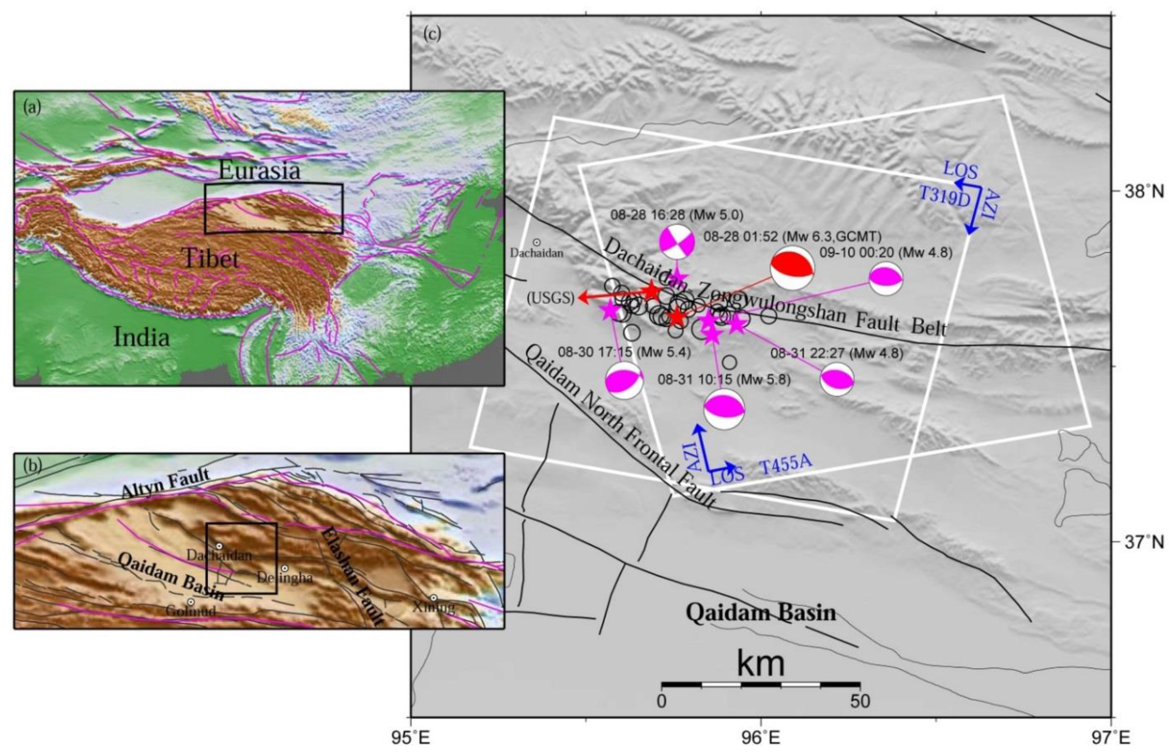
| Mainshock b | 08-28 01:52 | 95.760 | 37.640 | 101 | 60 | - | 12.0 g | 83 | - | 3.0 | 6.3 | |
| Aftershocks b | 08-28 16:28 | 95.760 | 37.750 | 56 | 80 | - | 17.0g | −3 | - | 0.035 | 5.0 | |
| 08-30 17:15 | 95.570 | 37.660 | 272 | 45 | - | 16.8g | 118 | - | 0.141 | 5.4 | ||
| 08-31 10:15 | 95.860 | 37.590 | 98 | 57 | - | 12.0 g | 90 | - | 0.562 | 5.8 | ||
| 08-31 22:27 | 95.930 | 37.620 | 107 | 45 | - | 12.0 g | 94 | - | 0.018 | 4.8 | ||
| 09-10 00:20 | 95.850 | 37.630 | 91 | 55 | - | 15.7 g | 84 | - | 0.018 | 4.8 | ||
2. InSAR Data Processing and Coseismic Deformation
2.1. InSAR Data Processing
| Track | Date 1 (yyyymmdd) | Date 2 (yyyymmdd) | Days a | Bperp b (m) | Σ c (cm) | L d (km) | |
|---|---|---|---|---|---|---|---|
| Descending | 319 | 20090114 | 20090916 | 19 | 222.02 | 0.52 | 3.84 |
| Ascending | 455 | 20090508 | 20091030 | 63 | 180.30 | 0.48 | 4.66 |

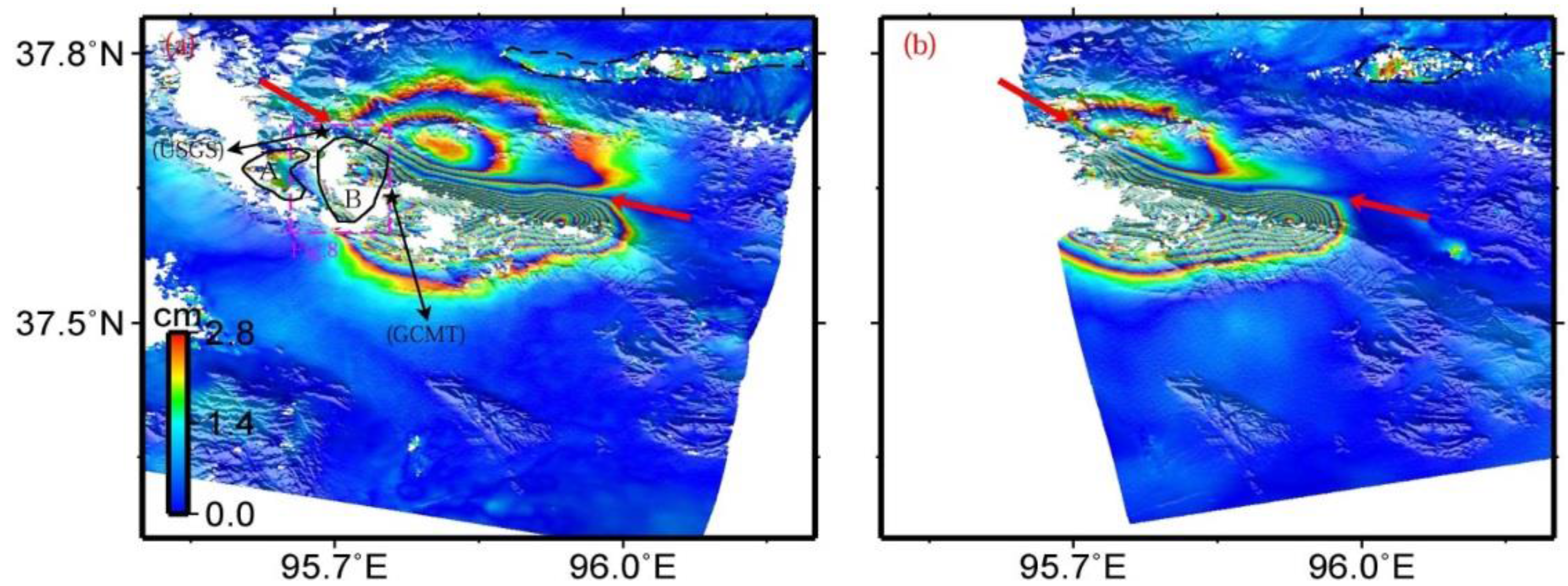
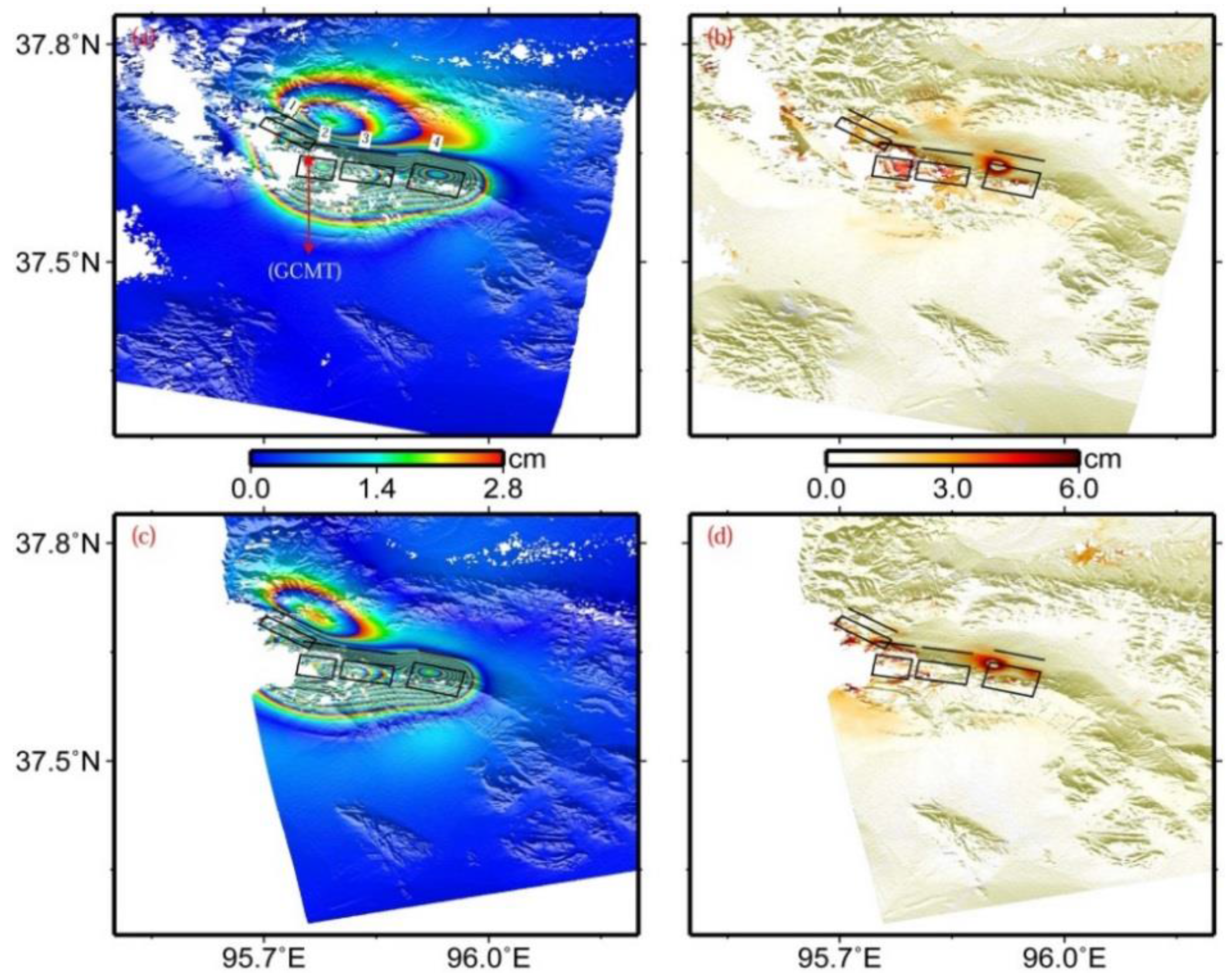
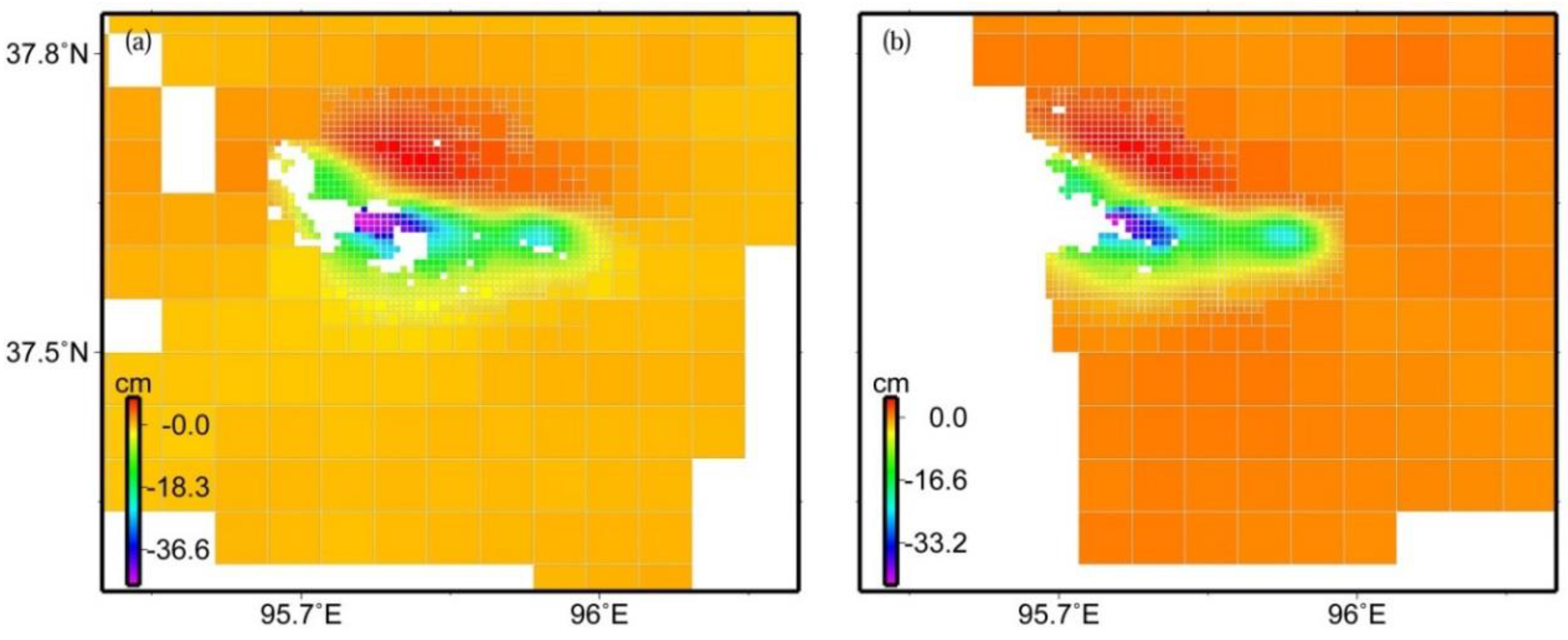
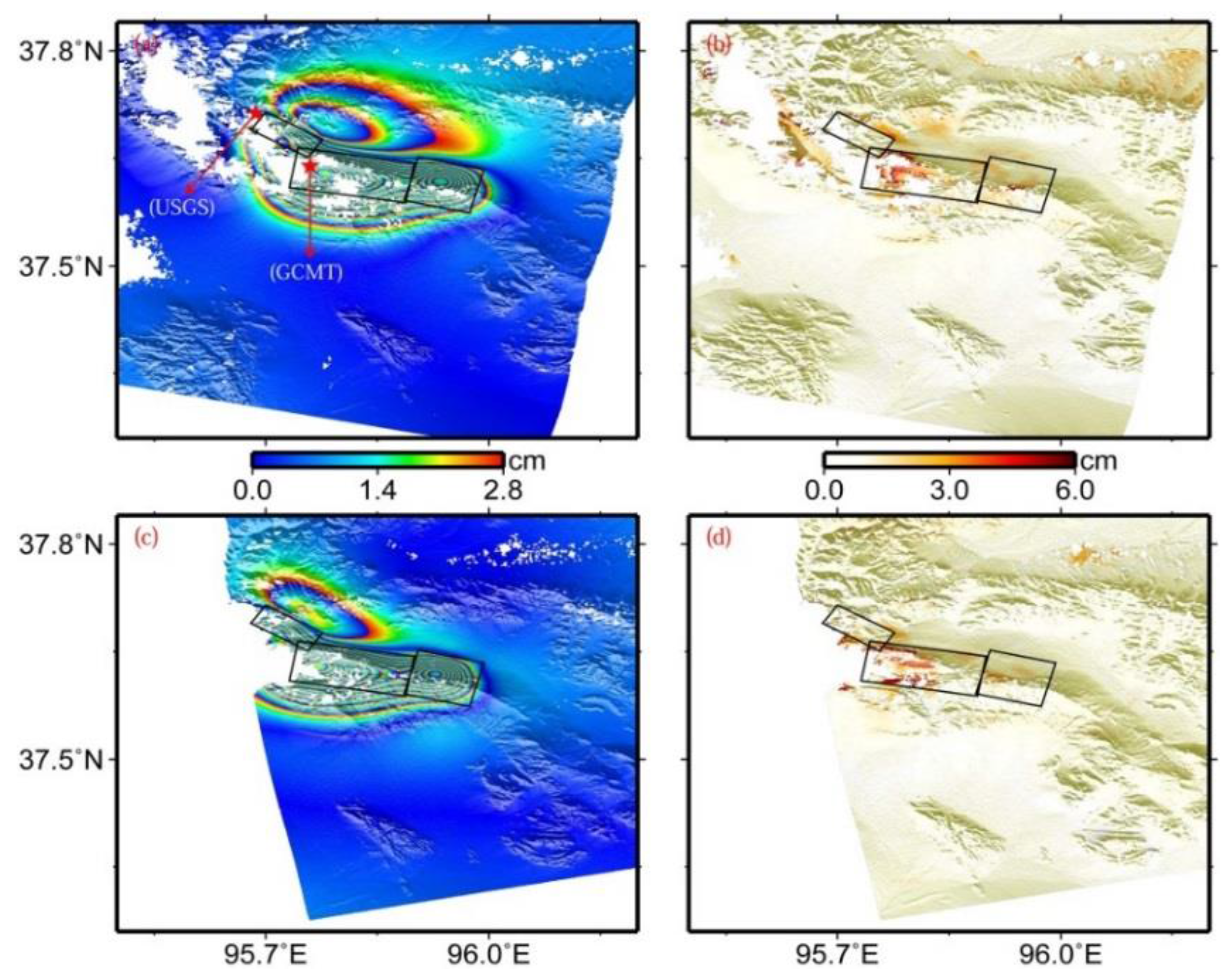
2.2. Coseismic Deformation
3. Inversion for Source Models
3.1. Fault Geometry Determination

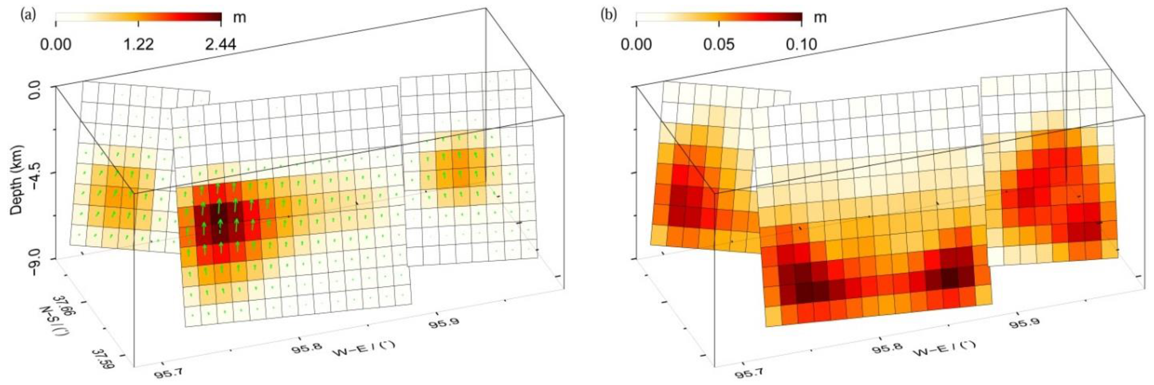
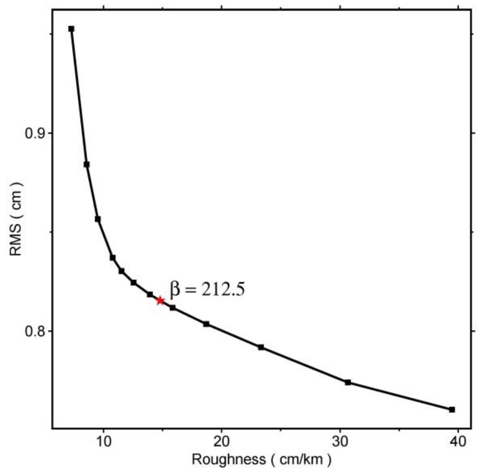
3.2. Slip Distribution Inversion

4. Discussions
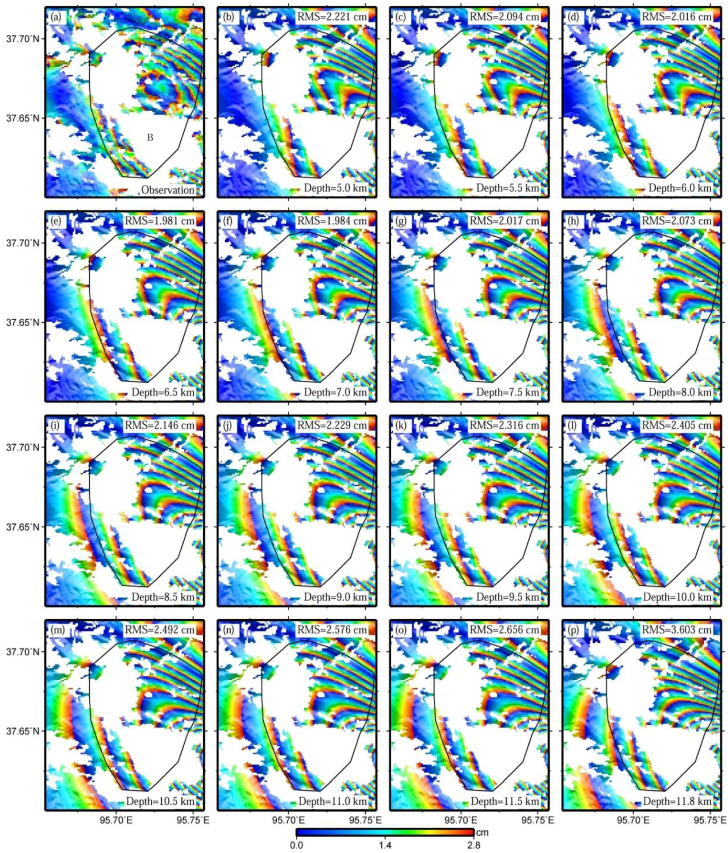
4.1. Rupture Depth of the 2009 Mw 6.3 Event
4.2. Rupture Propagation of the 2009 Mw 6.3 Event
4.3. Tectonic Implications of the 2009 Mw 6.3 Event
5. Conclusions
Acknowledgments
Author Contributions
Conflicts of Interest
References
- USGS. Available online: http://earthquake.usgs.gov/earthquakes/eqinthenews/2009/us2009kwaf/ (accessed on 17 May 2015).
- GCMT. Available online: http://www.globalcmt.org/cmtsearch.html (accessed on 17 May 2015).
- Deng, Q.; Zhang, P.; Ran, Y.; Yang, X.; Min, W.; Chu, Q. Basic characteristics of active tectonics of China. Sci. Chin. Ser. D 2003, 46, 356–372. [Google Scholar]
- Zhang, P.; Deng, Q.; Zhang, G.; Ma, J.; Gan, W.; Min, W.; Mao, F.; Wang, Q. Active tectonic blocks and strong earthquakes in the continent of China. Sci. Chin. Ser. D 2003, 46, 13–24. [Google Scholar]
- Elliott, J.; Parsons, B.; Jackson, J.; Shan, X.; Sloan, R.; Walker, R. Depth segmentation of the seismogenic continental crust: the 2008 and 2009 Qaidam earthquakes. Geophys. Res. Lett. 2011, 38, L06305. [Google Scholar] [CrossRef]
- Liu, W.; Wang, P.; Ma, Y.; Chen, Y. Relocation of Dachaidan Ms 6.4 earthquake sequence in Qinghai province in 2009 using the double difference location method. Plateau Earthq. Res. 2011, 23, 24–26. [Google Scholar]
- Segall, P.; Davis, J.L. GPS applications for geodynamics and earthquake studies. Annu. Rev. Earth Planet. Sci. 1997, 25, 301–336. [Google Scholar] [CrossRef]
- Massonnet, D.; Rossi, M.; Carmona, C.; Adragna, F.; Peltzer, G.; Feigl, K.; Rabaute, T. The displacement field of the Landers earthquake mapped by radar interferometry. Nature 1993, 364, 138–142. [Google Scholar] [CrossRef]
- Feigl, K.L.; Sergent, A.; Jacq, D. Estimation of an earthquake focal mechanism from a satellite radar interferogram: application to the December 4, 1992 Landers aftershock. Geophys. Res. Lett. 1995, 22, 1037–1040. [Google Scholar] [CrossRef]
- Wright, T.J. Remote monitoring of the earthquake cycle using satellite radar interferometry. Phil. Trans. R. Soc. Lond. A 2002, 360, 2873–2888. [Google Scholar] [CrossRef] [PubMed]
- Wang, R.; Xia, Y.; Grosser, H.; Wetzel, H.-U.; Kaufmann, H.; Zschau, J. The 2003 Bam (SE Iran) earthquake: precise source parameters from satellite radar interferometry. Geophys. J. Int. 2004, 159, 917–922. [Google Scholar] [CrossRef]
- Hu, J.; Li, Z.-W.; Ding, X.-L.; Zhu, J.-J. Two-dimensional co-seismic surface displacements field of the Chi-Chi earthquake inferred from SAR image matching. Sensors 2008, 8, 6484–6495. [Google Scholar] [CrossRef]
- Kotsis, I.; Kontoes, C.; Paradissis, D.; Karamitsos, S.; Elias, P.; Papoutsis, I. A methodology to validate the InSAR derived displacement field of the September 7th, 1999 Athens earthquake using terrestrial surveying. improvement of the assessed deformation field by interferometric stacking. Sensors 2008, 8, 4119–4134. [Google Scholar] [CrossRef]
- Zhang, L.; Wu, J.; Ge, L.; Ding, X.; Chen, Y. Determining fault slip distribution of the Chi-Chi Taiwan earthquake with GPS and InSAR data using triangular dislocation elements. J. Geodyn. 2008, 45, 163–168. [Google Scholar] [CrossRef]
- Zhou, X.; Chang, N.-B.; Li, S. Applications of SAR interferometry in earth and environmental science research. Sensors 2009, 9, 1876–1912. [Google Scholar] [CrossRef] [PubMed]
- Tong, X.; Sandwell, D.T.; Fialko, Y. Coseismic slip model of the 2008 Wenchuan earthquake derived from joint inversion of interferometric synthetic aperture radar, GPS, and field data. J. Geophys. Res. 2010, 115, B04314. [Google Scholar] [CrossRef]
- Qiao, X.; Yang, S.; Du, R.; Ge, L.; Wang, Q. Coseismic slip from the 6 October 2008, Mw 6.3 Damxung earthquake, Tibetan Plateau, constrained by InSAR observations. Pure Appl. Geophys. 2011, 168, 1749–1758. [Google Scholar] [CrossRef]
- Weston, J.; Ferreira, A.M.; Funning, G.J. Global compilation of interferometric synthetic aperture radar earthquake source models: 1. comparisons with seismic catalogs. J. Geophys. Res. 2011, 116, B08408. [Google Scholar] [CrossRef]
- Zha, X.; Dai, Z. Constraints on the seismogenic faults of the 2003–2004 Delingha earthquakes by InSAR and modeling. J. Asian Earth Sci. 2013, 75, 19–25. [Google Scholar] [CrossRef]
- Kaneko, Y.; Hamling, I.; Van Dissen, R.; Motagh, M.; Samsonov, S. InSAR imaging of displacement on flexural-slip faults triggered by the 2013 Mw 6.6 Lake Grassmere earthquake, central New Zealand. Geophys. Res. Lett. 2015, 42, 781–788. [Google Scholar] [CrossRef]
- Motagh, M.; Bahroudi, A.; Haghighi, M.H.; Samsonov, S.; Fielding, E.; Wetzel, H.-U. The 18 August 2014 Mw 6.2 Mormori, Iran, earthquake: a thin-skinned faulting in the Zagros Mountain inferred from InSAR measurements. Seismol. Res. Lett. 2015, 86, 775–782. [Google Scholar] [CrossRef]
- Okada, Y. Surface deformation due to shear and tensile faults in a half-space. Bull. Seismol. Soc. Am. 1985, 75, 1135–1154. [Google Scholar]
- Peltzer, G.; Saucier, F. Present-day kinematics of Asia derived from geologic fault rates. J. Geophys. Res. 1996, 101, 27943–27956. [Google Scholar] [CrossRef]
- Wright, T.J.; Lu, Z.; Wicks, C. Source model for the Mw 6.7, 23 October 2002, Nenana Mountain earthquake (Alaska) from InSAR. Geophys. Res. Lett. 2003, 30, 1974. [Google Scholar] [CrossRef]
- Liu, Y.; Xu, C.; Wen, Y.; He, P.; Jiang, G. Fault rupture model of the 2008 Dangxiong (Tibet, China) Mw 6.3 earthquake from Envisat and ALOS data. Adv. Space Res. 2012, 50, 952–962. [Google Scholar] [CrossRef]
- Rosen, P.A.; Hensley, S.; Peltzer, G.; Simons, M. Updated repeat orbit interferometry package released. Eos Trans. AGU 2004, 85, 47. [Google Scholar] [CrossRef]
- Farr, T.G.; Rosen, P.A.; Caro, E.; Crippen, R.; Duren, R.; Hensley, S.; Kobrick, M.; Paller, M.; Rodriguez, E.; Roth, L.; et al. The shuttle radar topography mission. Rev. Geophys. 2007, 45, RG2004. [Google Scholar] [CrossRef]
- Goldstein, R.M.; Werner, C.L. Radar interferogram filtering for geophysical applications. Geophys. Res. Lett. 1998, 25, 4035–4038. [Google Scholar] [CrossRef]
- Goldstein, R.; Zebker, H.; Werner, C. Satellite radar interferometry: two-dimensional phase unwrapping. Radio Sci. 1988, 23, 713–720. [Google Scholar] [CrossRef]
- Hanssen, R.F. Radar Interferometry: Data Interpretation and Error Analysis; Kluwer Academic Publishers: Dordrecht, the Netherlands, 2001; Volume 2, p. 301. [Google Scholar]
- Ding, X.; Li, Z.; Zhu, J.; Feng, G.; Long, J. Atmospheric effects on InSAR measurements and their mitigation. Sensors 2008, 8, 5426–5448. [Google Scholar] [CrossRef]
- Xu, C.; Liu, Y.; Wen, Y.; Wang, R. Coseismic slip distribution of the 2008 Mw 7.9 Wenchuan earthquake from joint inversion of GPS and InSAR data. Bull. Seismol. Soc. Am. 2010, 100, 2736–2749. [Google Scholar] [CrossRef]
- Wen, Y.; Xu, C.; Liu, Y.; Jiang, G.; He, P. Coseismic slip in the 2010 Yushu earthquake (China), constrained by wide-swath and strip-map InSAR. Nat. Hazards Earth Syst. Sci. 2013, 13, 35–44. [Google Scholar] [CrossRef]
- Jónsson, S.; Zebker, H.; Segall, P.; Amelung, F. Fault slip distribution of the 1999 Mw 7.1 Hector Mine, California, earthquake, estimated from satellite radar and GPS measurements. Bull. Seismol. Soc. Am. 2002, 92, 1377–1389. [Google Scholar] [CrossRef]
- Li, Z.; Elliott, J.R.; Feng, W.; Jackson, J.A.; Parsons, B.E.; Walters, R.J. The 2010 Mw 6.8 Yushu (Qinghai, China) earthquake: constraints provided by InSAR and body wave seismology. J. Geophys. Res. 2011, 116, B10302. [Google Scholar] [CrossRef]
- Clarke, P.; Paradissis, D.; Briole, P.; England, P.; Parsons, B.; Billiris, H.; Veis, G.; Ruegg, J.C. Geodetic investigation of the 13 May 1995 Kozani-Grevena (Greece) earthquake. Geophys. Res. Lett. 1997, 24, 707–710. [Google Scholar] [CrossRef]
- Jiang, G.; Xu, C.; Wen, Y.; Liu, Y.; Yin, Z.; Wang, J. Inversion for coseismic slip distribution of the 2010 Mw 6.9 Yushu earthquake from InSAR data using angular dislocations. Geophys. J. Int. 2013, 194, 1011–1022. [Google Scholar] [CrossRef]
- Funning, G.J.; Parsons, B.; Wright, T.J.; Jackson, J.A.; Fielding, E.J. Surface displacements and source parameters of the 2003 Bam (Iran) earthquake from Envisat advanced synthetic aperture radar imagery. J. Geophys. Res. 2005, 110, B09406. [Google Scholar] [CrossRef]
- Lasserre, C.; Peltzer, G.; Cramp, F.; Klinger, Y.; Van der Woerd, J.; Tapponnier, P. Coseismic deformation of the 2001 Mw = 7.8 Kokoxili earthquake in Tibet, measured by synthetic aperture radar interferometry. J. Geophys. Res. 2005, 110, B12408. [Google Scholar] [CrossRef]
- Ma, Y.; Liu, W.; Wang, P.; Yang, X.; Chen, Y. Characteristics and anomaly of earthquake sequence activity of Dachaidan Ms 6.3 and Ms 6.4 in 2008 and 2009. Earthq. Res. Chin. 2012, 28, 188–199. [Google Scholar]
- Chen, S.; Xu, F.; Peng, D. Characteristics of basement structures and their controls on hydrocarbon in Qaidam Basin. Xinjiang Pet. Geol. 2000, 21, 175–179. [Google Scholar]
- Jiang, B.; Xu, F.; Peng, D.; Zhou, J.; Jin, F. Deformation characteristics of fault structures on the northern fringe of Qaidam Basin. J. Chin. Univ. Min. Technol. 2004, 33, 687–792. [Google Scholar]
- Xiong, S.; Ding, Y.; Li, Z. Characteristics of China continent magnetic basement depth. Chin. J. Geophys. 2014, 57, 3981–3993. [Google Scholar]
- Wessel, P.; Smith, W.H. New, Improved Version of Generic Mapping Tools Released. Eos Trans. AGU 1998, 79, 579–579. [Google Scholar] [CrossRef]
© 2015 by the authors; licensee MDPI, Basel, Switzerland. This article is an open access article distributed under the terms and conditions of the Creative Commons Attribution license (http://creativecommons.org/licenses/by/4.0/).
Share and Cite
Liu, Y.; Xu, C.; Wen, Y.; Fok, H.S. A New Perspective on Fault Geometry and Slip Distribution of the 2009 Dachaidan Mw 6.3 Earthquake from InSAR Observations. Sensors 2015, 15, 16786-16803. https://doi.org/10.3390/s150716786
Liu Y, Xu C, Wen Y, Fok HS. A New Perspective on Fault Geometry and Slip Distribution of the 2009 Dachaidan Mw 6.3 Earthquake from InSAR Observations. Sensors. 2015; 15(7):16786-16803. https://doi.org/10.3390/s150716786
Chicago/Turabian StyleLiu, Yang, Caijun Xu, Yangmao Wen, and Hok Sum Fok. 2015. "A New Perspective on Fault Geometry and Slip Distribution of the 2009 Dachaidan Mw 6.3 Earthquake from InSAR Observations" Sensors 15, no. 7: 16786-16803. https://doi.org/10.3390/s150716786
APA StyleLiu, Y., Xu, C., Wen, Y., & Fok, H. S. (2015). A New Perspective on Fault Geometry and Slip Distribution of the 2009 Dachaidan Mw 6.3 Earthquake from InSAR Observations. Sensors, 15(7), 16786-16803. https://doi.org/10.3390/s150716786