In the preceding section, no error sources are taken into consideration, but as mentioned earlier, the body inertial frame components of and are derived by the measurements of accelerometers and FOG. Therefore, the effect of Inertial Measurement Unit (IMU) sensor errors and base motion should be taken into account. The analysis of error characteristics driven by IMU sensor errors and base motion is done in the following section. On the other hand, since the coarse alignment time is generally fixed, and is adjustable, the optimal ratio between median integration time and total integration time exists and is derived with the help of error analysis. Also, based on the previous analysis, the adequate selection of the most accurate algorithm for FOG INS according to the actual operational conditions is provided.
In practical implementation, the equation for
should be rewritten in the form:
where
and
represent computed noncollinear vectors, and are shown in
Table 3.
where
is calculated by:
denotes the measurement quantity measured by FOG, and can be expressed as:
where
is the FOG error. The other measurement quantity
can be represented as [
14,
15]:
Neglecting the second order small term, it can be simplified into:
where
is the external acceleration caused by linear motion,
represents the accelerometer error.
5.1. Error Sources Analysis
It is quite obvious from
Table 1 and
Table 3 that the elements of
are precisely known, but
contains sensor errors and base motion which are uncertain. The error analysis in this section utilizes perturbation methods, then
and
can be expanded in series and arranged in the following forms:
where
is the error matrix between
and
and the matrix
represents the departure of
from
.
Equation (21) shows that the error of
is caused by the departure of
from
. By comparing
Table 2 and
Table 3, we find that the matrix
results from the departure of
from
(
). This means that we can study the error sources by analyzing the departure of
from
. Consider Equation (18) and the following equation:
where
is the error matrix caused by the FOG error.
can be expressed as:
where products of error quantities have been neglected. Then the departure of
from
(
) can be obtained and described as follows (for the two alignment algorithms):
where
. Obviously, this departure is mainly caused by
,
, and
. It means that sensor errors
,
, and base motion
are the major error sources of the error matrix
.
5.2. The Effect of Sensor Errors
First, the effect of sensor errors is analyzed. In our analysis, we assume that the accelerometer errors are basically bias errors and the FOG errors are basically constant drifts. It is well known that the steady-state alignment errors are affected by the sensor errors. In general, the relationships between alignment errors and sensor errors are often expressed in the navigation frame because only the analysis of alignment errors in the navigation frame is meaningful, since the final results of alignment need to be expressed in the navigation frame. For many alignment approaches (for instance, gyrocompass alignment and optimum alignment), the relationships can be written as [
16,
17,
18,
19]:
where
is the east alignment error,
is the north alignment error,
is the up alignment error,
represents the east accelerometer error,
represents the north accelerometer error, and
represents the east FOG error. By utilizing the perturbation method, the correlation between
and
in this paper can be described as:
where
is the error matrix related to
,
, and
, and
denotes the error matrix of
. Since the local latitude
and time
are known,
is equal to zero. On the other hand, the error source of Equation (15) is only the FOG error, and the total alignment time is short, so the error matrix
in Equation (29) is small and can be ignored. It should be noted that the error matrix
in Equations (24) and (25) could not be neglected because the magnitude of the product between matrix
and gravity vector
is considerable.
Considering the previously analysis, Equation (29) is simplified into:
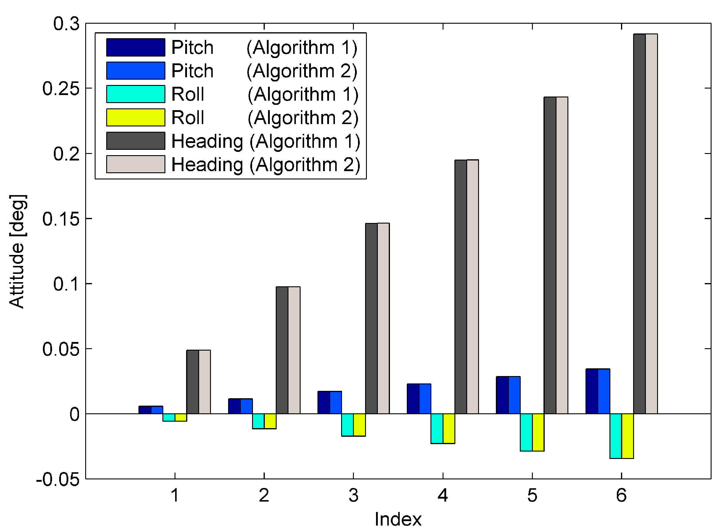
Evidently, and are equivalent and transformational, and then the effect of sensor errors on matrix can be transformed into the influence of sensor errors on matrix . In this paper, the relationships between alignment errors and sensor errors in the navigation frame for the two alignment algorithms are provided and can be expressed as Equations (26) and (27), and then the effect of sensor errors is uncorrelated with the integration time. This conclusion can be drawn from Simulation A, since the effect of sensor errors is deterministic. Both of these two alignment algorithms have the same accuracy under the condition of existing internal sensor errors, and it is verified in Simulation A.
5.3. Base Motion Effect and Optimal Parameter Design
Secondly, the effect of base motion is analyzed, and the optimal ratio between and is provided. In general, base motion typically falls into two categories. One is the angular motion, and the other is the linear motion. Fortunately, these two alignment algorithms are not influenced by angular motion; this conclusion can be drawn from Equations (24) and (25), and is verified in simulation B. Then the remaining problem is the analysis of the effect of linear motion on matrix , and this problem is resolved by utilizing the property of matrix norm.
Under the disturbance of linear motion, the departure of
from
(
) can be simplified into (for the two alignment algorithms):
where
, and it represents the position variation caused by linear motion
during
. From Equations (31) and (32), we find that the velocity variation is the influence factor for Algorithm 1, but for Algorithm 2, both the position variation and initial velocity are the influence factors.
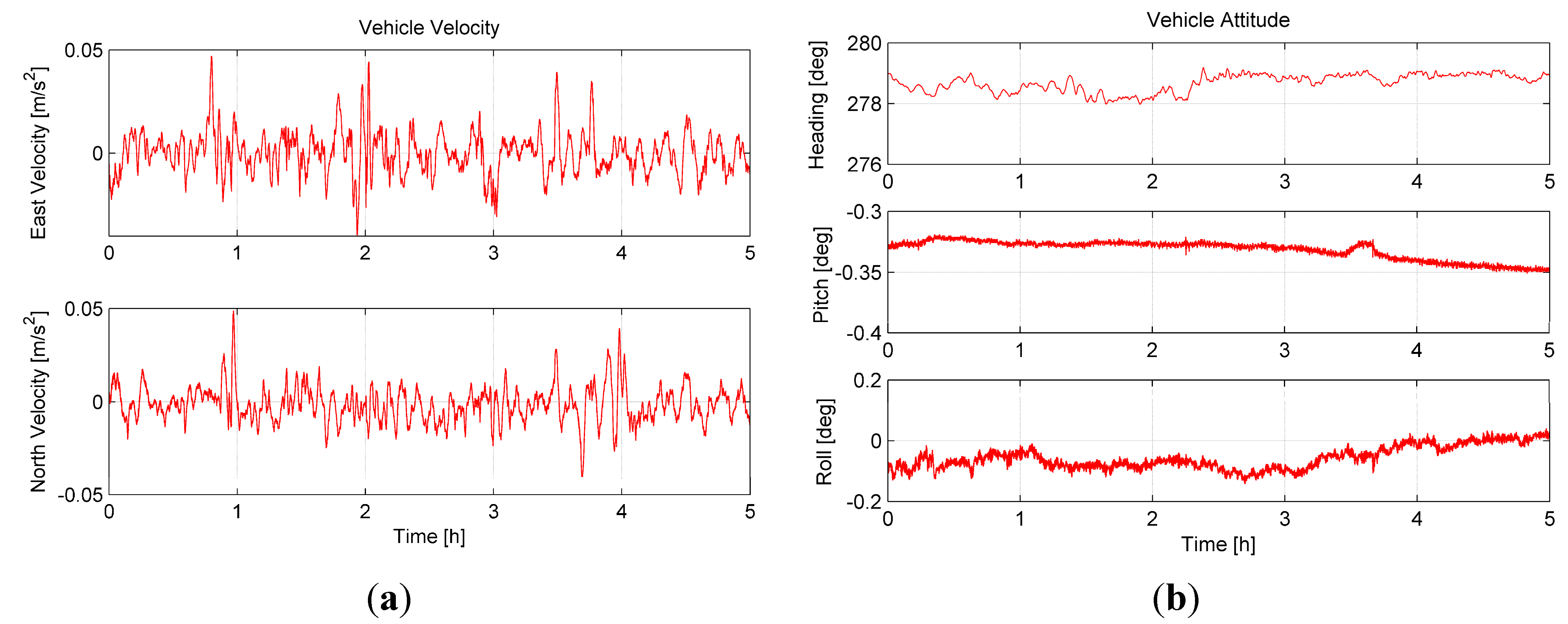
Coarse alignment is generally performed under quasi-stationary conditions, and they are characterized as having bounded position and attitude movement such as produced by wind gusts, passengers, and sea waves. The velocity and position variations are bounded, and both of them have same order of magnitude. Unfortunately, for Algorithm 2, the error caused by initial velocity is proportional to time, and this error is bigger than velocity and position variations in general. First, in order to simplify the analysis, the initial velocity is assumed to be compensated for Algorithm 2. After that, the effect of initial velocity is taken into consideration.
According to Equation (21), we have:
where
represents the Frobenious norm,
the detailed derivation of
can be seen in
Appendix A. It is important to notice that the norm of
determines the influence of linear motion on error matrix
. Evidently, the large norm of
leads to amplification of the linear motion influence; in contrast, the small norm of
leads to reducing the effect of linear motion on error matrix
. Now we consider the two alignment algorithms provided in
Section 4, and show how to get the specific expression for matrix norm
in the following.
5.3.1. Algorithm 1
Let us begin by substituting
and
into Equation (34), then the norm of matrix
can be rewritten as:
In Equation (35),
and
can be derived from Equation (B4) in
Appendix B, and expressed as:
But the norm of
is difficult to obtain directly. This problem is resolved in a practical manner by using the definition of the cross-product. According to its definition, we have:
where
is the angle between
and
, and the angular direction is defined by the right hand rule that curls the fingers of the right hand from
into
. Since the coarse alignment is generally accomplished within a short time (only few minutes), we assume that the vectors
,
, and
lie in the same plane. Then
can be obtained by:
where
is the angle between
and
,
is the angle between
and
.
and
can be drawn from Equation (C4) in
Appendix C, and expressed as:
Thus, Equation (35) transforms into:
It is obvious from Equation (42) that the norm of
for Algorithm 1 is obtained and determined by parameters
,
, and
. In other words, the influence of linear motion on error matrix
for Algorithm 1 is determined by parameters
,
, and
. During the previous derivation, the assumption that the three vectors
,
, and
lie in the same plane was made in order to simplify the derivation of
. Now, for the purpose of validating this assumption, simulations are conducted, and the results are shown in
Table 4. The simulation conditions are set as:
t0 = 0 s,
tk1 = 50 s,
tk2 = 120 s, and the linear velocity caused by the base motion is equal to zero.
Table 4.
The difference between calculated and actual .
Table 4.
The difference between calculated and actual .
| Latitude | Angle | Error |
|---|
| Actual Value | Calculated Value | Absolute Error | Relative Error |
|---|
| 0° | 0.1462° | 0.1462° | 0.0000° | 0.00% |
| 30° | 0.1266° | 0.1266° | 0.0000° | 0.00% |
| 45° | 0.1034° | 0.1034° | 0.0000° | 0.00% |
Simulation results show that for a short period of time, the difference between calculated and actual is negligible. Therefore, the previous assumption is correct.
5.3.2. Algorithm 2
Similar derivations to those of the last section lead us to get the norm of
for Algorithm 2. In this section,
and
need to be provided, and the assumption that the vectors
,
, and
lie in the same plane also should be made. Firstly,
and
are derived from Equation (D3) in
Appendix D, and expressed as:
Secondly, based on the previous assumption, the angle
between
and
is obtained as:
where
is the angle between
and
,
is the angle between
and
.
and
can be deduced from Equation (E4) in
Appendix E, and described as:
Obviously, the specific expression for the norm of
can be acquired from Equation (48), and it is also determined by parameters
,
, and
. Therefore, the influence of linear motion on error matrix
for Algorithm 2 is determined by parameters
,
, and
, too. In order to validate the assumption made in this section, simulations are performed, and the results are shown in
Table 5. The simulation conditions are set as:
t0 = 0 s,
tk1 = 50 s,
tk2 = 120 s, the linear velocity caused by the base motion is equal to zero.
Table 5.
The difference between calculated and actual .
Table 5.
The difference between calculated and actual .
| Latitude | Angle | Error |
|---|
| Actual Value | Calculated Value | Absolute Error | Relative Error |
|---|
| | | | |
| | | | |
| | | | |
Obviously, although the calculated value is not equal to the actual value, the difference between them is small. This means that the assumption made in this section is correct as well.
5.3.3. Optimal Parameter Design
From Equations (42) and (48), we find that both of the matrix norms for the two algorithms are determined by parameters
,
, and
. In operational situations, total integration time
is generally fixed, and the local latitude
is related to the position of the vehicle on which the FOG INS is mounted. Then, however, only parameter
is adjustable. Considering
,
, and by definition,
where
is the ratio between
and
,
, and
represents the duration time of coarse alignment. Equations (42) and (48) can be rewritten as:
Evidently, the matrix norms for the two algorithms are determined by parameter
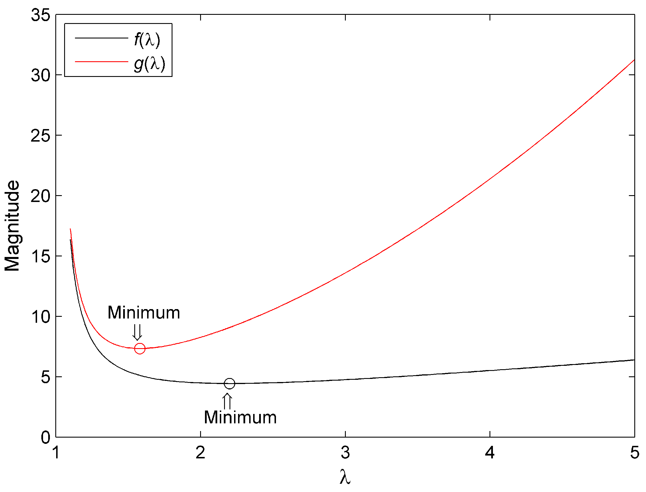
, and the optimal parameters for the two algorithms are achieved by minimizing the following functions, respectively:
Then the determination of optimal parameters is transformed into the solution of the minimum problem. The differential equations for
and
are provided as follows:
It is obvious from Equations (54) and (55) that
and
in the condition
. Therefore, the minimum will appear on the interval (1, 5). The graphs of functions
and
are drawn by Matlab, and shown in
Figure 2.
It can be seen from
Figure 2 that each of the functions has only one extreme point, and the extreme point is the minimum. Then by solving equations
and
, the optimal parameters for the two algorithms are obtained as:
The substitution of Equations (56) and (57) into Equations (50) and (51), the optimal norms of
, can be acquired as:
Figure 2.
The graphs of functions and .
Figure 2.
The graphs of functions and .
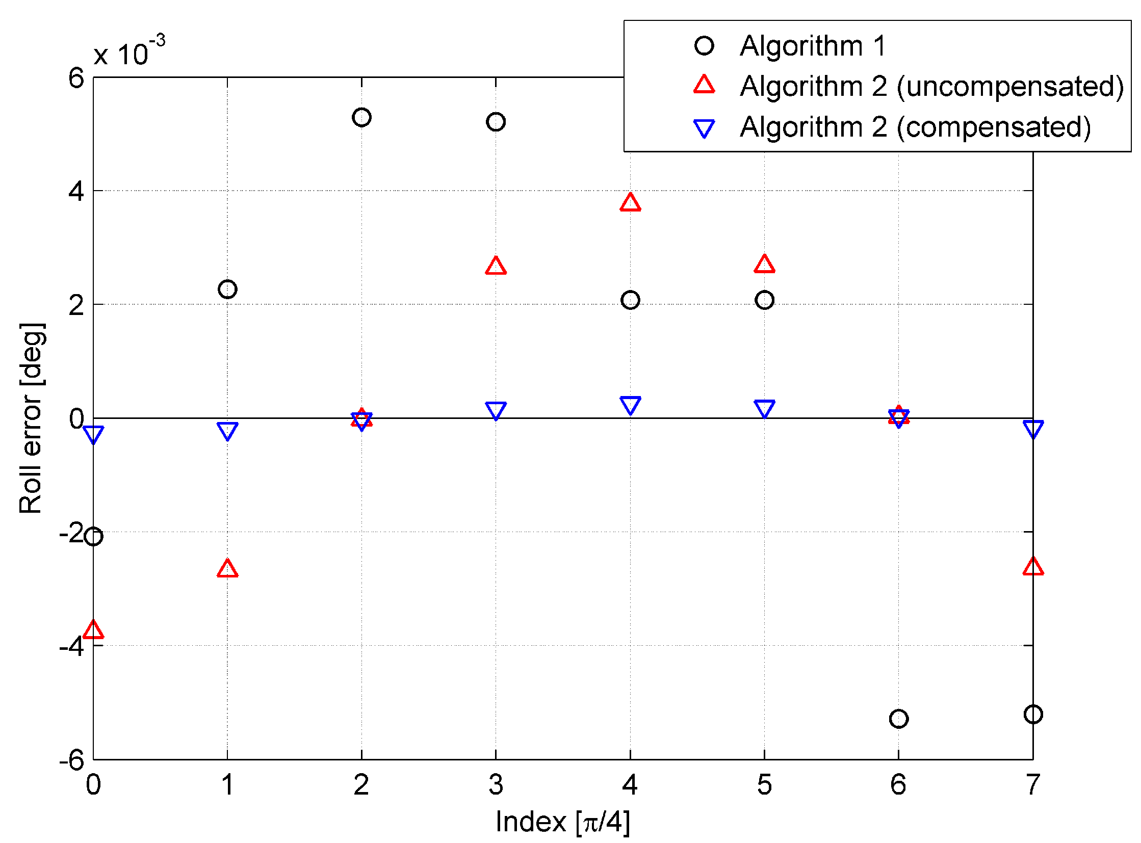
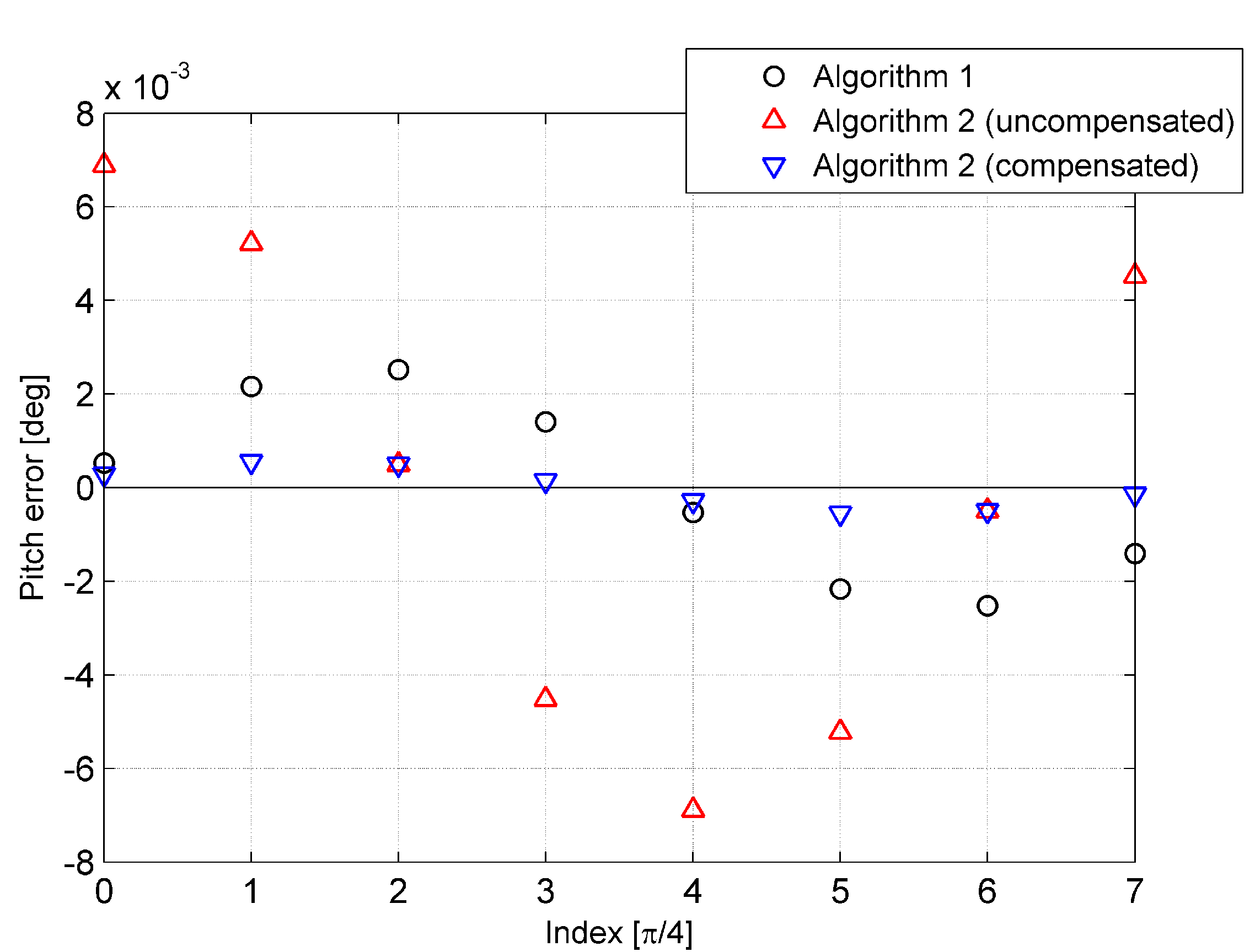
It is quite obvious that is smaller than due to , and this means that the performance of Algorithm 2 is better than that of Algorithm 1 under the disturbance of bounded errors. In order to validate the two optimal parameters provided by Equations (56) and (57), simulations are performed in Simulation C.
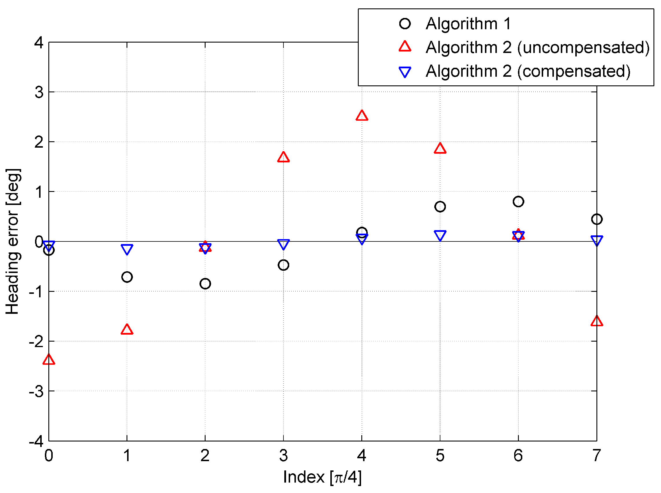
Alternately, if the error caused by initial velocity is uncompensated, the performance of Algorithm 2 will be worse than that of Algorithm 1, and a rough and direct explanation for this result is given in the following.
Considering the departure of
from
for Algorithm 2, the error caused by initial velocity can be expressed as:
Ignoring the departure of
from
, and then drawing
T from
, we have:
Equation (61) reflects the influence of initial velocity on error matrix for Algorithm 2. Since the magnitude of initial velocity is close to that of velocity variation, and the value of Equation (61) is bigger than that of Equation (56), we can draw the conclusion that the performance of Algorithm 2 is worse than that of Algorithm 1 while the error produced by initial velocity is uncompensated. This conclusion is verified in simulation D.
Summarizing, Equations (58), (59) and (61) allow us to make the adequate selection of the most accurate algorithm for coarse alignment according to the actual operational conditions. Algorithm 1 is suitable for Marine FOG INS, since the FOG INS is usually disturbed by sea waves and the initial velocity caused by waves is unknown. On the other hand, Algorithm 2 is appropriate for Vehicular FOG INS, because the FOG INS can generally keep stationary at the beginning of the coarse alignment in this operational condition, and then the initial velocity is equal to zero.


