4.1. Directivity Versus Spacing
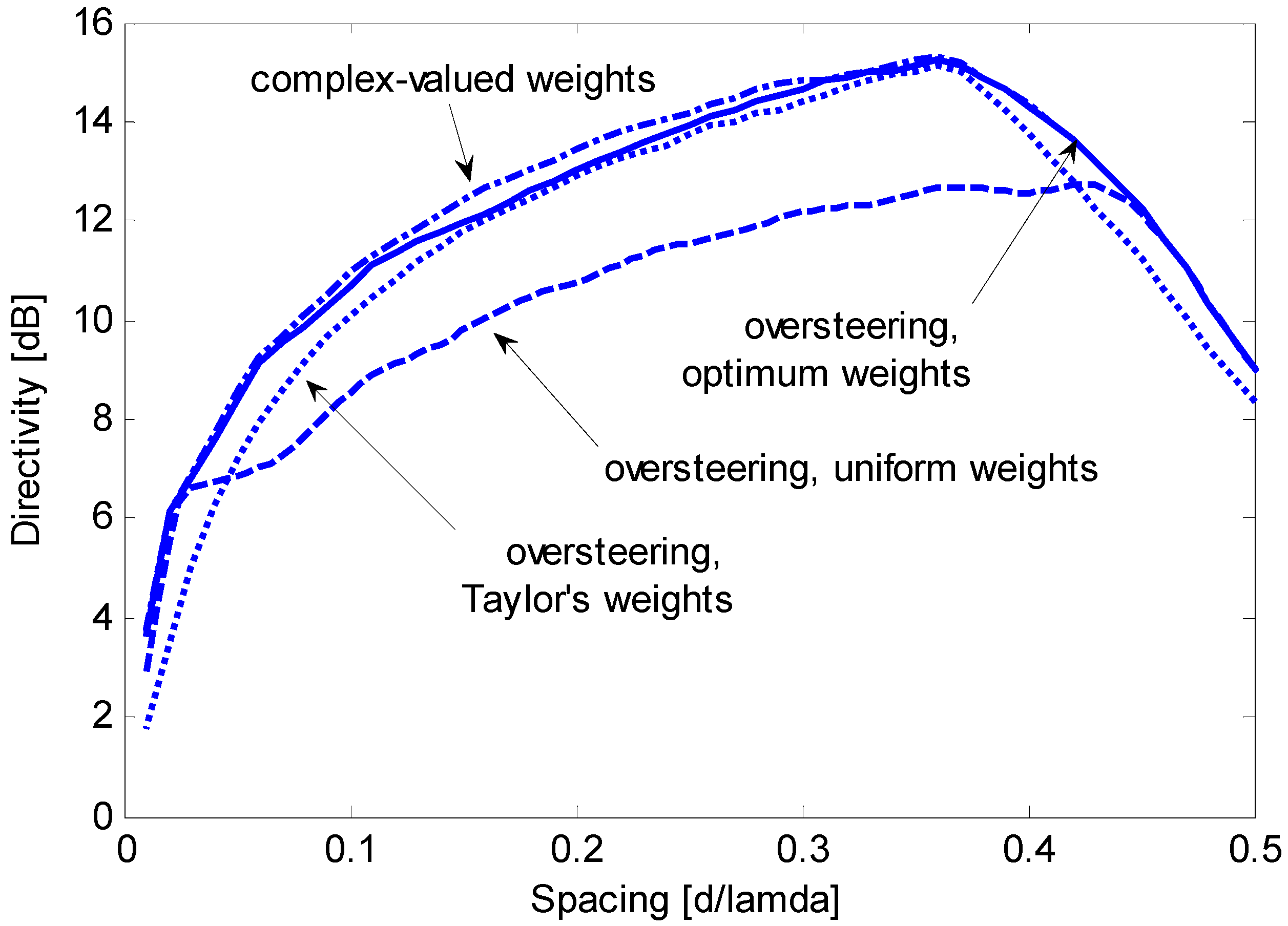
Initially, a linear array composed of eight ES sensors is considered, and the WNG is imposed to be always ≥ 0 dB. The directivity of this array is evaluated as a function of the normalized spacing (i.e., the ratio between d and λ, d/λ) considering spacing values smaller than λ/2. Regarding oversteering, three different real weighting windows are considered: uniform, Taylor’s, and the optimum window computed by solving Equation (28).
First, we assess the performance of the end-fire array without oversteering when complex or real weight coefficients are used. For a given value of
d/λ, the optimum complex weights are computed by setting ε = 0 and solving Equation (23). The optimum real weights are computed by setting ε = 0 and solving Equation (28). CVX software is employed for convex programming [
20] on a common PC equipped with an Intel
® Core i5 CPU with 2.60 GHz of clock and 12 Gbyte of RAM, and the solution is found in less than 0.2 s.
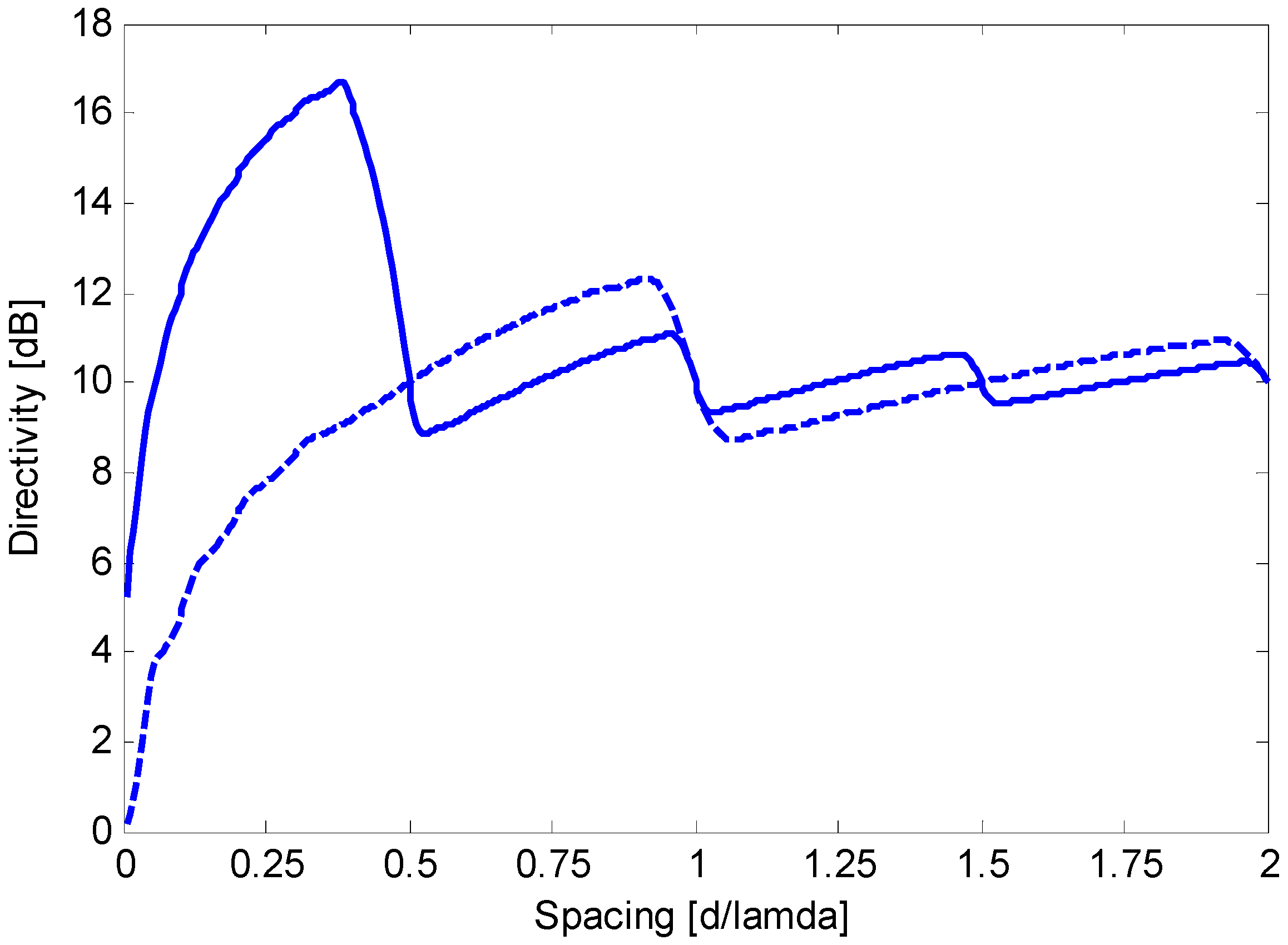
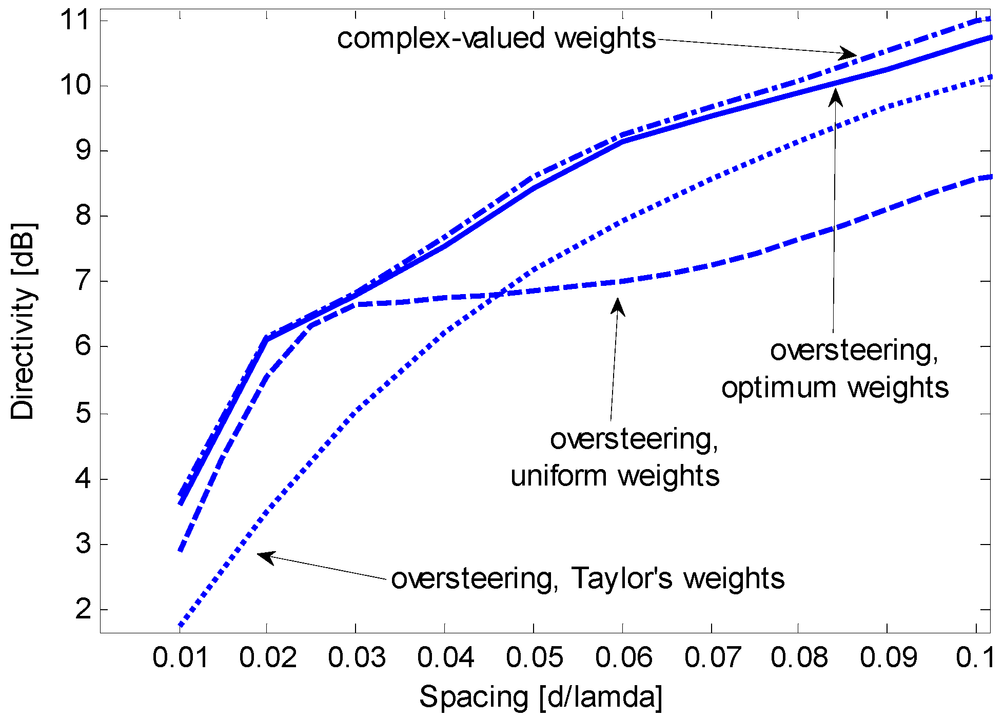
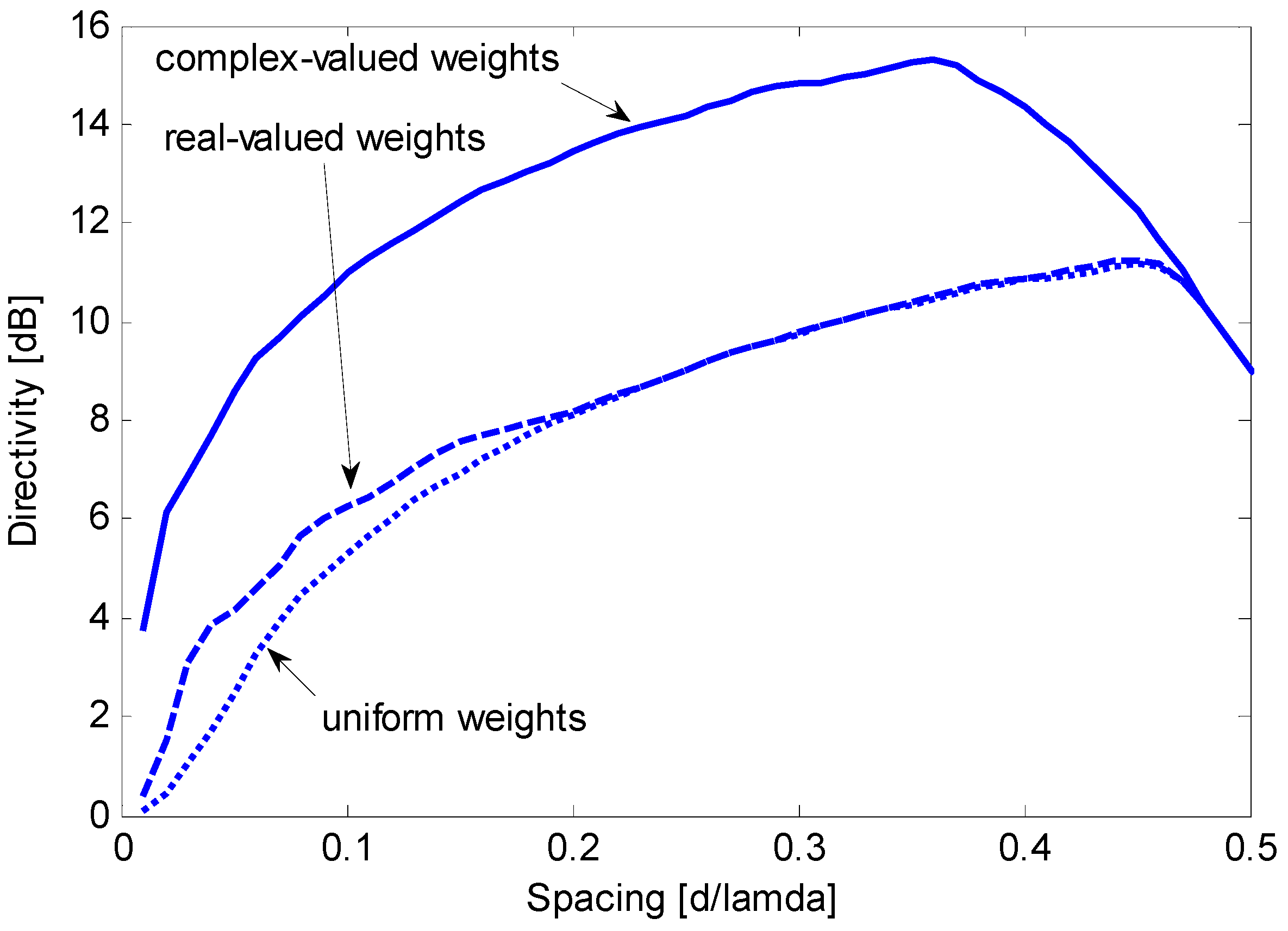
Figure 4 compares the maximum constrained directivities and illustrates the directivity obtainable with uniform weights. In this specific case, the optimum real weights only provide a directivity higher than that obtained by uniform weights for
d/λ < 0.22, with a gain that does not exceed 2 dB. In contrast, the complex weights provide a directivity gain of approximately 5 dB over a wide interval of
d/λ. The absolute maximum constrained directivity is obtained for
d/λ = 0.36 and has a value of 15.3 dB. Because 10 log(
N) is 9 dB and 10 log(
N2) is 18 dB, the optimum complex weights allow for a robust directivity with an absolute maximum that is significantly higher than
N and moderately lower than
N2.
Figure 5 compares the performances obtained by the oversteering technique when the uniform and Taylor’s weighting windows are applied. The optimum value for the oversteering amount ε, where ε ϵ (0, λ/
d − 2), is computed by the algorithm described in
Section 3.3 using a predefined weight vector (uniform or Taylor’s) instead of
woR(ε
z). A discretization step for ε of 0.01 is established and a Matlab
® script is run on the previously mentioned PC, which results in a computation time that does not exceed 5 s.
Figure 4.
Maximum constrained directivity obtained for an end-fire array of N = 8 sensors by imposing WNG ≥ 0 dB using complex weights (solid line) or real weights (dashed line); the directivity obtained using uniform weights (dotted line) is included for comparison.
Figure 4.
Maximum constrained directivity obtained for an end-fire array of N = 8 sensors by imposing WNG ≥ 0 dB using complex weights (solid line) or real weights (dashed line); the directivity obtained using uniform weights (dotted line) is included for comparison.
Figure 5.
Maximum constrained directivity obtained for an end-fire array of N = 8 sensors by imposing WNG ≥ 0 dB using the oversteering technique with uniform weights (solid line) and Taylor’s weights (dotted line); the performance obtained without oversteering using optimum real weights is included for comparison (dashed line).
Figure 5 shows that the oversteering technique performs better than the optimum real weights without oversteering. In particular, Taylor’s window provides advantageous directivity values over a wide interval of
d/λ, from 0.05 to approximately 0.42. According to
Figure 4 and
Figure 5, the performance achieved by real weights (uniform or optimized) without oversteering is poorer than the performance achieved by complex weights or by the oversteering technique; as a result, real weights without oversteering will be disregarded in subsequent investigations. The latter is intended to assess the oversteering with the real weights that maximize the constrained directivity. For a given value of
d/λ, the oversteering optimization and the weight computation are performed by the algorithm described in
Section 3.3. A discretization step for ε of 0.01 is established, and CVX software is employed for convex programming [
20] on the previously mentioned PC, which results in a computation time that does not exceed 4 min.
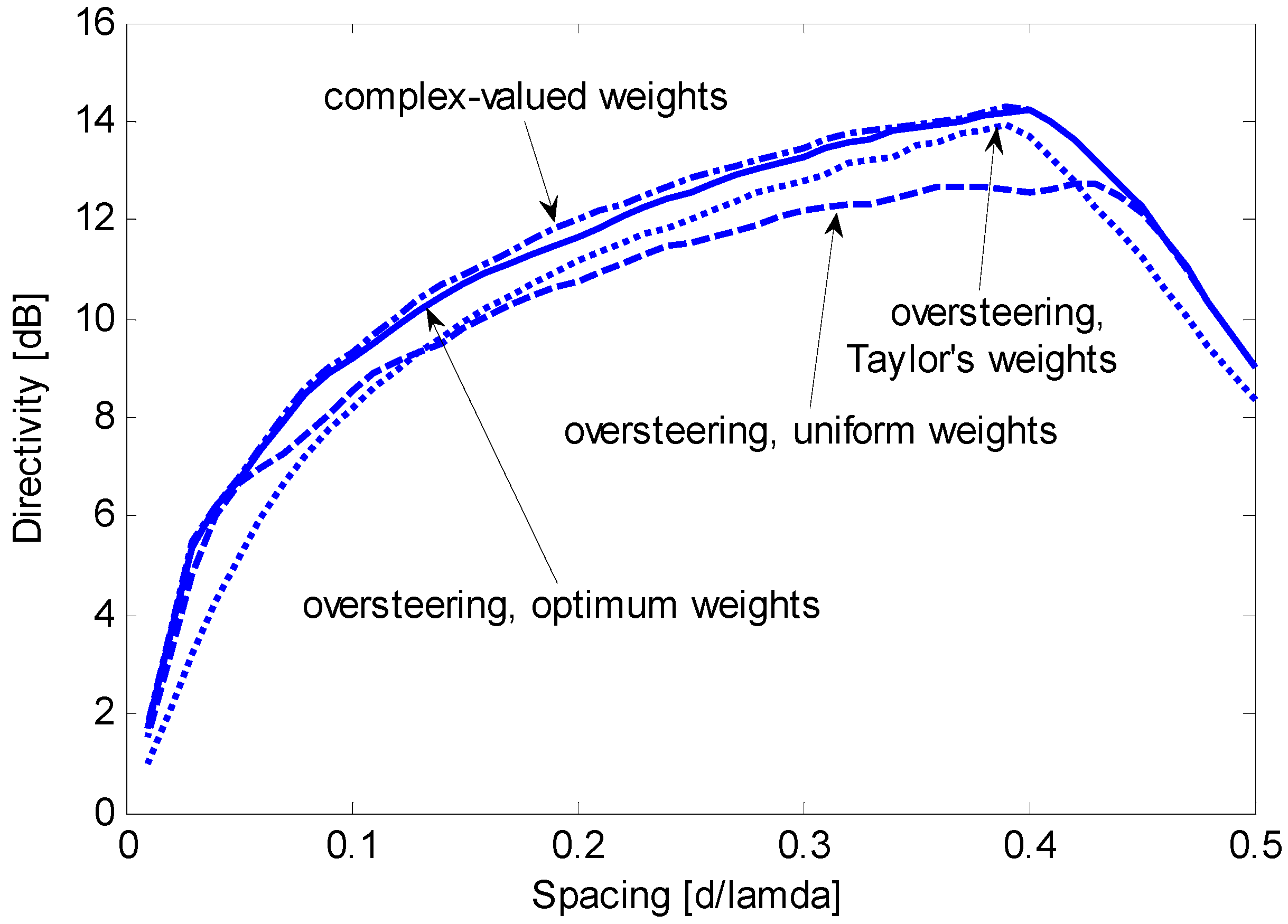
Figure 6 presents the maximum constrained directivities obtained with the oversteering technique using three weighting windows: uniform, Taylor’s, and optimized. The absolute maximum for the constrained directivity (
i.e., the performance obtained with the optimum complex weights) is also included for comparison. It is possible to verify that the optimum real-valued weights always provide the best oversteering performance and that the achieved directivity is very close or equal to the absolute maximum. Although the Taylor’s weights provide results that are only slightly poorer over a significant interval of
d/λ (from approximately 0.1 to 0.4), the optimized weights ensure the achievement of the maximum constrained directivity achievable by the oversteering technique. In this specific case, for values of
d/λ lower than 0.1, the optimized weights provide a significant advantage over traditional weighting windows. To realize this fact,
Figure 7 presents a magnification of a portion of
Figure 6.
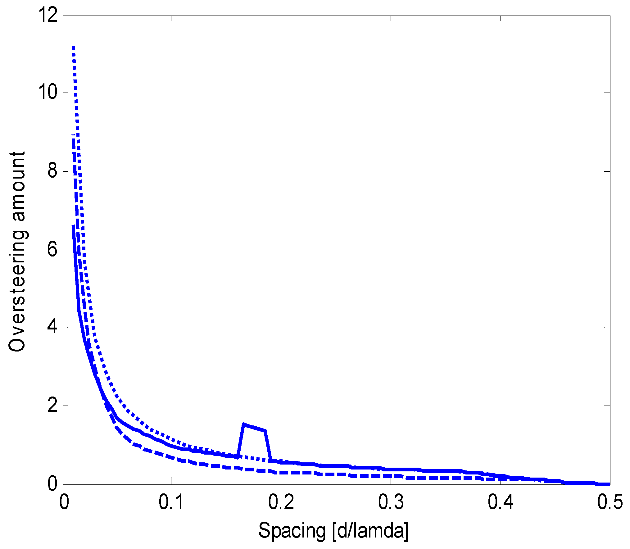
Figure 8 presents the oversteering amount ε required to obtain the maximum constrained directivity using uniform, Taylor’s, and optimized weights. In general, the oversteering amount ε necessary to achieve the maximum directivity increases as the spacing
d decreases and the allowed interval for ε increases. When
d/λ is less than 0.04, the optimized weights achieve the maximum constrained directivity using an oversteering amount that is smaller than those with uniform and Taylor’s weights. Thus, unlike oversteering with traditional weights, the proposed optimization performs best when considering both the oversteering amount and weighting window.
Figure 6.
Maximum constrained directivity obtained for an end-fire array of N = 8 sensors by imposing WNG ≥ 0 dB using the oversteering technique with optimum weights (solid line), uniform weights (dashed line), and Taylor’s weights (dotted line); the performance without oversteering obtained with optimum complex weights is included for comparison (dash-dotted line).
Figure 7.
Magnification of a section from
Figure 6.
Figure 7.
Magnification of a section from
Figure 6.
Figure 8.
Oversteering amount, ε, that provides the maximum constrained directivity for an end-fire array of N = 8 transducers, which is obtained by imposing WNG ≥ 0 dB for three weighting windows: optimum weights (solid line), uniform weights (dashed line), and Taylor’s weights (dotted line).
Figure 8.
Oversteering amount, ε, that provides the maximum constrained directivity for an end-fire array of N = 8 transducers, which is obtained by imposing WNG ≥ 0 dB for three weighting windows: optimum weights (solid line), uniform weights (dashed line), and Taylor’s weights (dotted line).
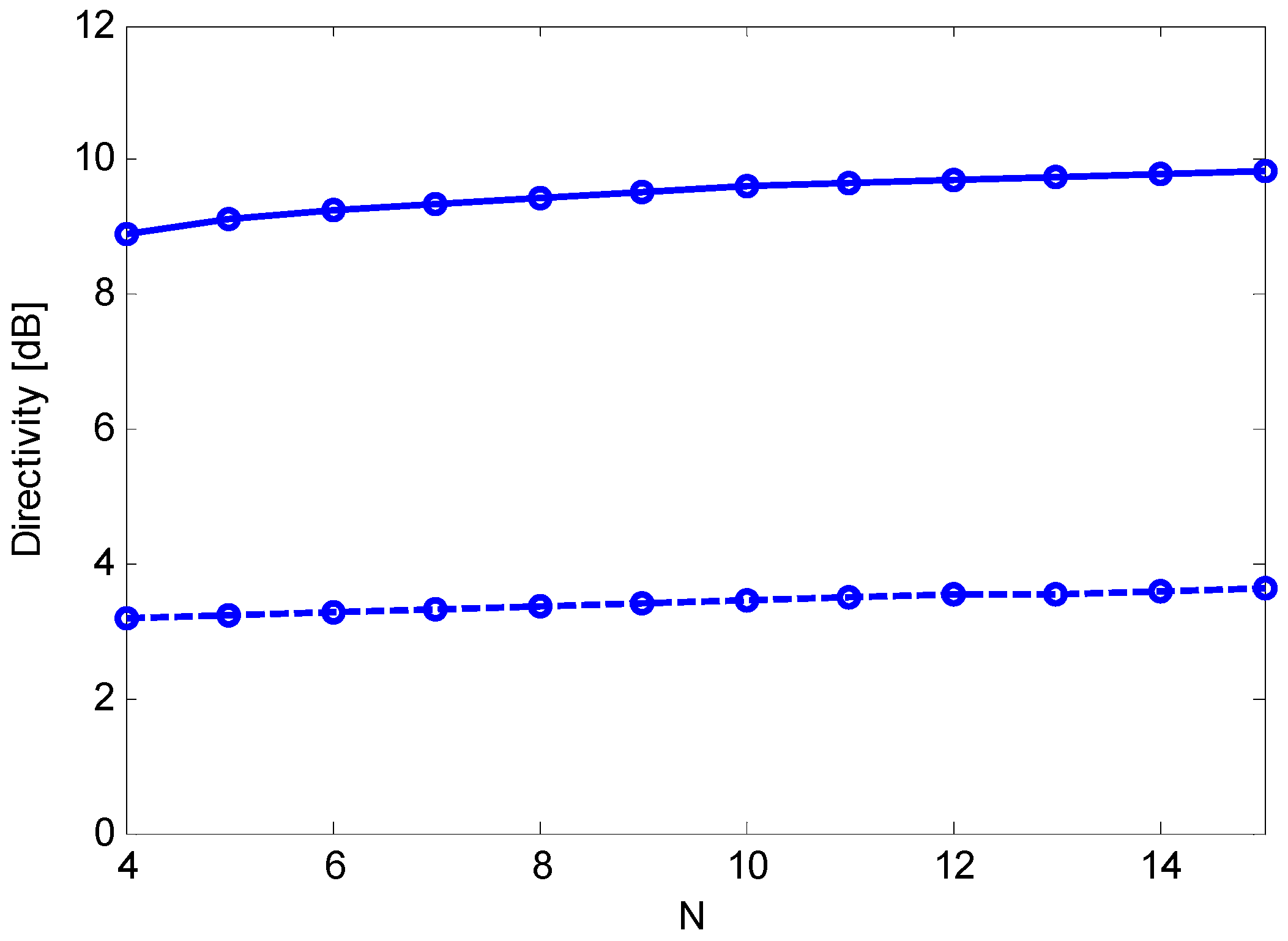
An assessment of the oversteering performance with respect to the number of array sensors is shown in
Figure 9, where the same comparison as
Figure 6 is repeated for
N = 4 (
Figure 9a) and
N = 16 (
Figure 9b). The computation times do not change considerably with respect to the aforementioned values (a moderate increase is observed also if the number of array sensor becomes greater than 16). With both four and 16 sensors, the oversteering with optimized weights yields almost the same directivity as the optimum complex weights over the entire spacing domain. Where a difference is visible, it does not exceed 0.6 dB. Oversteering with Taylor’s and uniform weights does not guarantee the same performance level: for
N = 4, both weighting windows yield a constrained directivity that is approximately 2 dB lower than the best constrained directivity over large intervals of the spacing domain; for
N = 16, Taylor’s window performs generally well but exhibits a 2-dB fall at the lower bound of the spacing domain, whereas the uniform weights yield a directivity that is approximately 3 dB lower than the best constrained directivity over a large portion of the spacing domain.
Figure 9.
Maximum constrained directivity obtained for end-fire arrays of (a) N = 4 and (b) N = 16 sensors by imposing WNG ≥ 0 dB for the oversteering technique with optimum weights (solid line), uniform weights (dashed line), and Taylor’s weights (dotted line); the performance obtained without oversteering using optimum complex weights is included for comparison (dash-dotted line).
For N = 4 and N = 16 (as well as for N = 8), the oversteering with optimum weights allows for a robust directivity with an absolute maximum that is significantly higher than N and moderately lower than N2. The spacing value at which the maximum directivity is obtained approaches 0.5 λ as N increases.
A final assessment considers robustness against mismatches of the sensor characteristics. A more severe bound can be imposed if the robustness provided by a WNG ≥ 0 dB is not sufficient.
Figure 10 presents the same comparison as
Figure 6 for the case when the WNG is imposed to be greater than 5 dB. In this case, the maximum achievable directivity is generally 1–2 dB lower than that obtained by imposing WNG ≥ 0 dB. Although the performance graphs are now closer to each other, the oversteering with optimum weights is still the only technique that yields a constrained directivity very similar to that of the optimum complex weights over the entire spacing domain. The absolute maximum of the constrained directivity is now obtained for
d/λ = 0.39 and has a value of 14.3 dB (compared to 15.3 dB obtained imposing WNG ≥ 0 dB). Because a WNG of 5 dB ensures a very robust design (for an eight-element array, the absolute maximum of the WNG is 9 dB), we conclude that, in this extreme case, the oversteering with optimum weights also provides a robust directivity with an absolute maximum between
N and
N2.
Figure 10.
Maximum constrained directivity obtained for an end-fire array of N = 8 sensors by imposing WNG ≥ 5 dB for the oversteering technique with optimum weights (solid line), uniform weights (dashed line), and Taylor’s weights (dotted line); the performance obtained without oversteering using optimum complex weights is included for comparison (dash-dotted line).
4.2. System Implementation
An analysis of Equation (7) reveals that for any ES linear array, the signal delays used with the oversteering technique differ from each other by an integer multiple of the quantity Δ, defined as follows:
Thus, if the sampling frequency fs is set to 1/Δ or to an integer multiple of 1/Δ, all of the delays to be applied to the received signals can be implemented in an easy and exact manner by shifting the signal of a given number of samples. Thus, before the beamforming sum, each signal should be multiplied by a real gain factor and shifted by an integer number of samples.
To verify the viability of this procedure, we can consider a linear array of microphones spaced 3.4 cm each other, working at a nominal frequency of 3.4 kHz (i.e., d = 0.34 λ). In this case, the microphone signals should be sampled at a frequency equal to or lower than 10 kHz, depending on the value of ε.
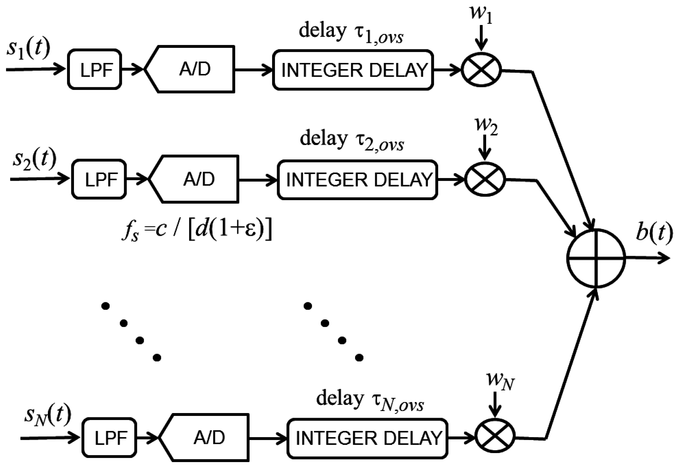
Figure 11 displays a schematic of the implementation of this beamforming technique. After low-pass filtering (LPF) to avoid aliasing, the
N input signals are digitized through analog-to-digital (A/D) converters that sample at a frequency
fs = 1/Δ =
c/[
d(1 + ε)]. If
fs is lower than the Nyquist rate, an integer multiple of
fs can be set as the sampling frequency. The
nth delay τ
n,ovs given in Equation (7) can be obtained very efficiently by shifting the
nth signal by a given number of samples using a digital integer delay line. Before performing the final sum that generates the output signal
b(
t), the
nth signal is multiplied by the real weight coefficient
wn. If optimum oversteering performance is desired, the weights
wn should be computed by solving Equation (28). Otherwise, the weights can be derived from a traditional weighting window, such as Taylor’s window.
Figure 11.
Schematic of oversteered end-fire beamformer for a suitable sampling frequency fs.
Figure 11.
Schematic of oversteered end-fire beamformer for a suitable sampling frequency fs.
The same simple implementation cannot be applied for the complex weights because the term φn in Equation (6) depends on the index n. The implementation of end-fire beamforming with complex weights requires the precise implementation of delays that are not integer multiples of the sampling period or the transformation of the received signals in their analytic versions and the processing of complex signals. Both these options are more involved than the implementation of the oversteered end-fire array, needing a processing architecture that requires additional money, resources, and space.
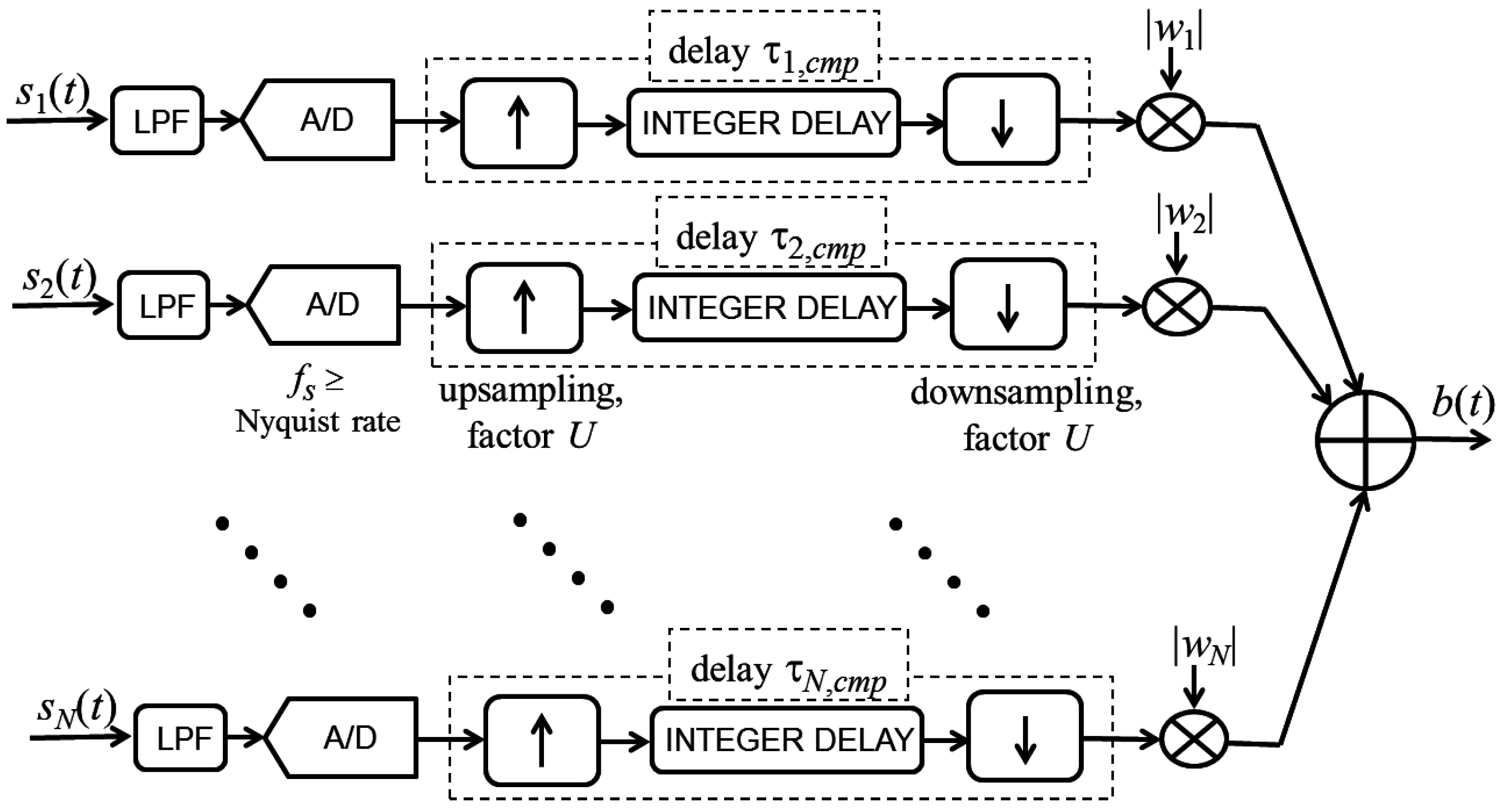
Of the two options for conducting end-fire beamforming with complex weights, the use of real signals is most similar to oversteering. This beamforming technique is mathematically defined in Equation (3), and a potential implementation scheme is shown in
Figure 12. After low-pass filtering (LPF) to avoid aliasing, the
N input signals are digitized through analog-to-digital (A/D) converters that sample at a frequency
fs, which is greater than or equal to the Nyquist rate. Unlike the oversteering case, the deployment of the delays τ
n,cmp given in Equation (6) requires digital fractional delay lines. For each signal, the commonly used implementation scheme includes an interpolator that upsamples the signal by a suitable factor
U, an integer delay line that approximates τ
n,cmp by shifting the signal by a given number of samples at the higher rate, and a decimator that downsamples the signal by the factor
U. Before performing the final sum that generates the output signal
b(
t), the
nth signal should be multiplied by the modulus of the complex weight coefficient
wn. To achieve the maximum constrained directivity, the weights
wn should be computed by solving Equation (23). An alternative to using the interpolator and decimator is to sample and process the input signals directly at the higher rate (
i.e.,
fsU). However, the example described in the next subsection demonstrates that such a sampling rate is much higher than that required for the oversteering case.
The comparison of
Figure 11 and
Figure 12 and consideration of the previously mentioned observations confirm that the implementation of the end-fire beamformer with complex weights is more complicated than the implementation of the oversteered beamformer.
Figure 12.
Schematic of end-fire beamformer using complex weights, where delays are implemented using digital fractional delay lines.
Figure 12.
Schematic of end-fire beamformer using complex weights, where delays are implemented using digital fractional delay lines.
4.3. Simulated Testing of an Array Design
To test the performance of the beamformers considered in this paper, we consider a linear array of eight microphones spaced 2.5 cm apart. We consider that a plane wave with a frequency of 680 Hz impinges on the array at an arrival angle that varies from −90° to 90°. Random mismatches among the microphone responses are introduced according to specified statistics. For each arrival angle, the electrical signals produced by the array sensors are digitized and processed according to the schematics shown in
Figure 11 and
Figure 12. The energy of the obtained beam signal is used to compose the actual beam power pattern |
Ba(
u)|
2 of the simulated array.
At a frequency of 680 Hz, the inter-element spacing
d is equal to 0.05 λ; thus, the nominal array performance for a WNG greater than or equal to 0 dB is as follows.
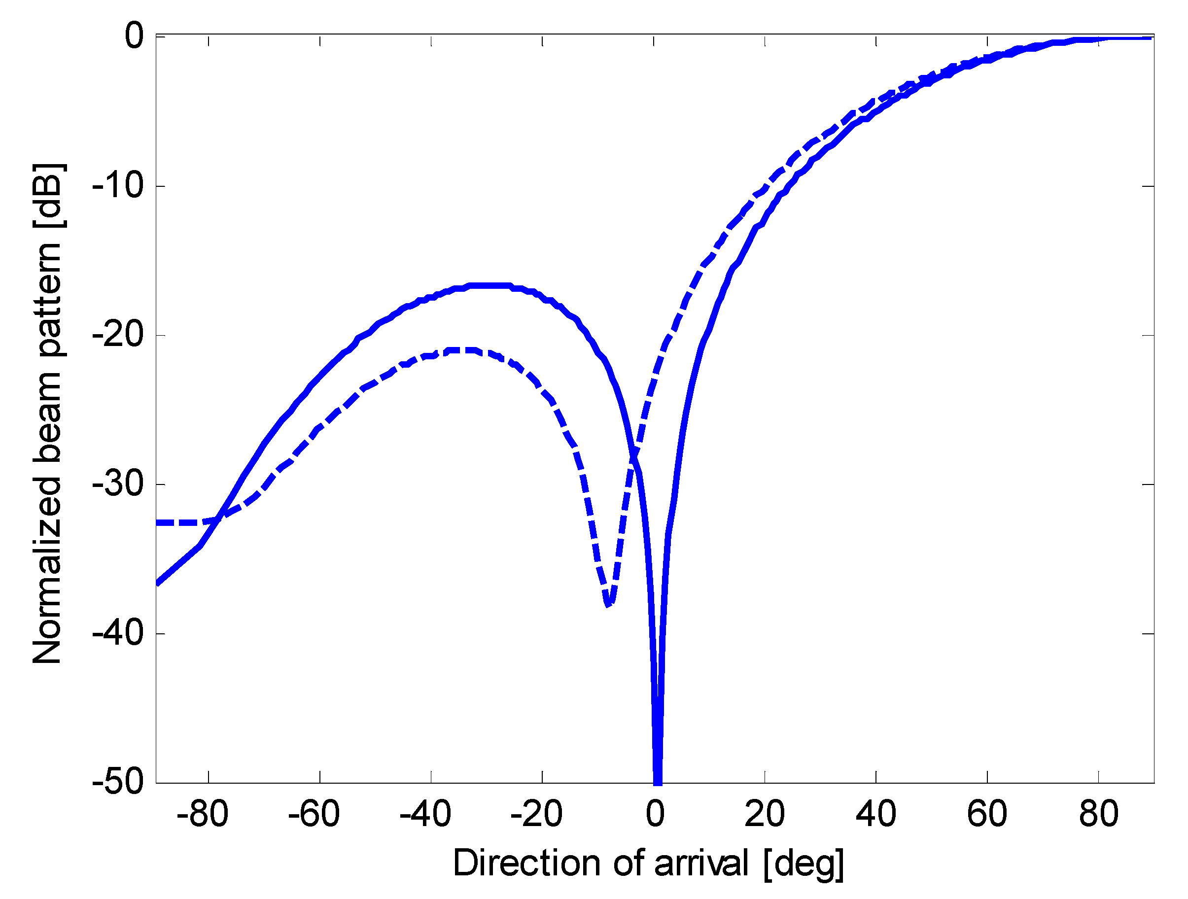
Figure 7 shows that the maximum constrained directivity is 8.62 dB using complex weights and 8.43 dB for oversteering using optimized weights. In the latter case,
Figure 8 shows that the oversteering amount should be ε = 1.71. For comparison, if oversteering is used with Taylor’s weights, the maximum constrained directivity is 7.20 dB and is achieved for an oversteering amount ε = 2.25. The nominal beam patterns for these three options are shown in
Figure 13,
Figure 14 and
Figure 15.
The performance is assessed using two subsequent tests: in the first test, the sampling frequency (and the upsampling factor) needed to achieve an actual beam pattern close to the nominal beam pattern is determined. In the second test (see the following subsection), a statistical investigation is used to assess the robustness of the beamforming performance against mismatches in the sensor responses.
In the first test, to clearly determine the relation between the sampling frequency and the beam pattern accuracy requires the assumption of ideal microphones (
i.e., sensors with perfectly matched responses) and the use of a metric for the beam pattern distortion. The metric is developed by introducing the percentage error ∑, which is defined as the normalized distance between the actual beam power pattern |
Ba(
u)|
2 and the nominal beam power pattern |
B(
u)|
2:
Obviously, both of the beam power patterns that are substituted into this equation must to be normalized functions.
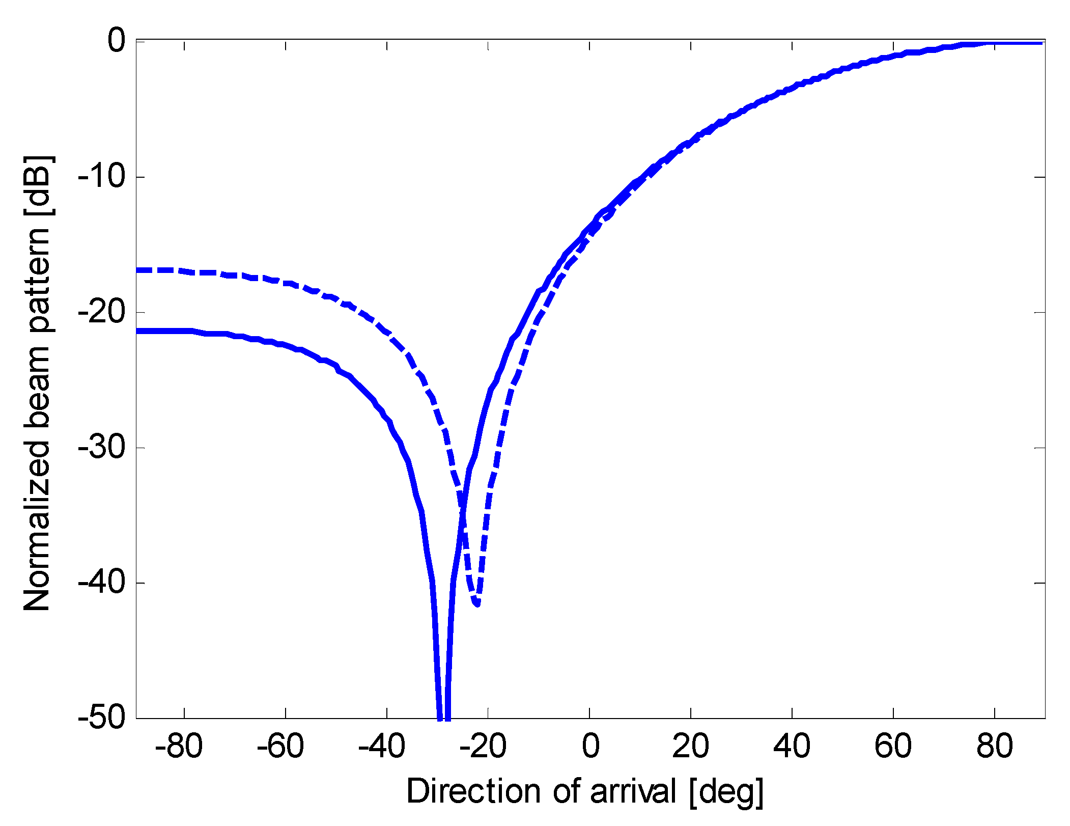
Figure 13.
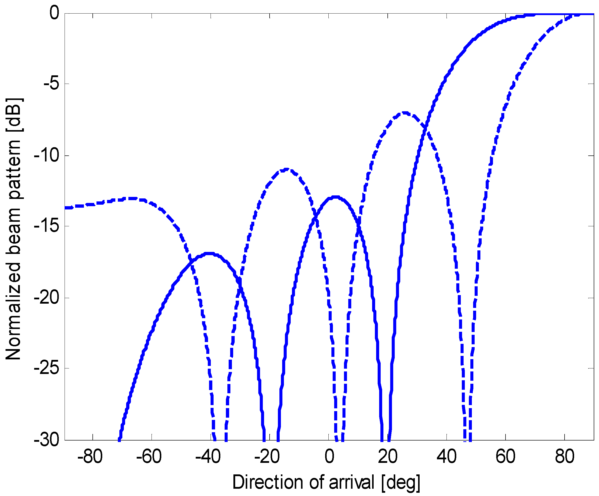
Nominal beam pattern (solid line) and actual beam pattern (dashed line) for beamforming with optimum complex weights applied to an end-fire array of eight microphones.
Figure 13.
Nominal beam pattern (solid line) and actual beam pattern (dashed line) for beamforming with optimum complex weights applied to an end-fire array of eight microphones.
Figure 14.
Nominal beam pattern (solid line) and actual beam pattern (dashed line) for oversteered beamforming with optimum real weights applied to an end-fire array of eight microphones.
Figure 14.
Nominal beam pattern (solid line) and actual beam pattern (dashed line) for oversteered beamforming with optimum real weights applied to an end-fire array of eight microphones.
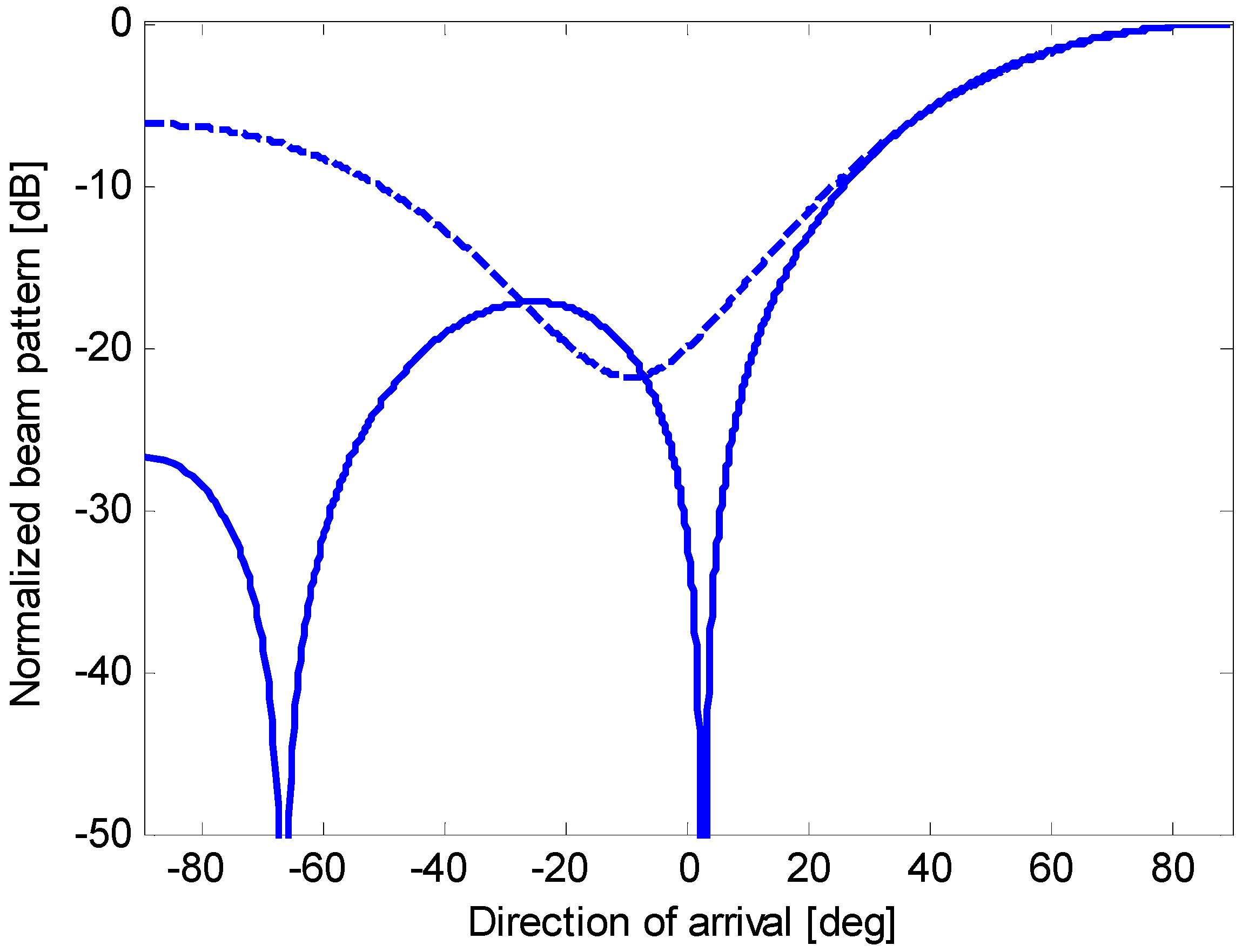
Figure 15.
Nominal beam pattern (solid line) and actual beam pattern (dashed line) for oversteered beamforming with Taylor’s weights applied to an end-fire array of eight microphones.
Figure 15.
Nominal beam pattern (solid line) and actual beam pattern (dashed line) for oversteered beamforming with Taylor’s weights applied to an end-fire array of eight microphones.
The oversteering amount that optimizes the performance should be used to set the sampling frequency
fs = 5.018 kHz for the oversteered beamforming with optimized weights. Using this specific value of
fs for the processing outlined in
Figure 11 results in an actual beam pattern that is identical to the nominal beam pattern. However, it is not necessary to acquire exactly 5018 samples per second to obtain good results: for instance, if the sampling frequency is set to 5 kHz or 5.05 kHz, the percentage error, ∑, does not exceed 1.9%. Similar conclusions are obtained for oversteered beamforming using Taylor’s weights. A zero error is obtained for a sampling frequency of 4.185 kHz; however, at frequencies around this value, the beam pattern is not significantly altered.
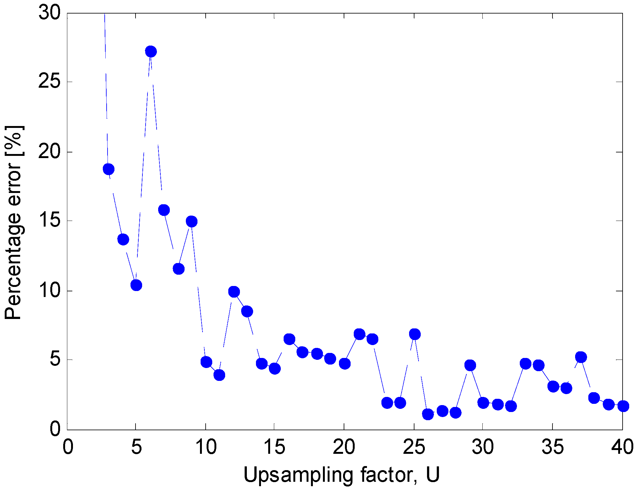
Figure 16.
Distortion of beam pattern (measured in terms of the percentage error ∑) for beamforming with optimum complex weights versus the upsampling factor U.
Figure 16.
Distortion of beam pattern (measured in terms of the percentage error ∑) for beamforming with optimum complex weights versus the upsampling factor U.
For beamforming using optimum complex weights, a sampling frequency
fs = 1.5 kHz is set that is slightly higher than the Nyquist rate.
Figure 16 shows the measured percentage error, ∑, when the upsampling factor
U is increased up to 40. To obtain an error, ∑, that is lower than 5%, an upsampling factor
U = 10 is necessary. Instead, if an error, ∑, lower than 2% is desired, the minimum upsampling factor is
U = 23. If a sampling frequency similar to the sampling frequency of the oversteered case is adopted without upsampling (
i.e.,
fs = 5 kHz and
U = 1), an error ∑equal to 22.7% is achieved and the actual beam pattern exhibits major distortions, as shown in
Figure 17.
Figure 17.
Nominal beam pattern (solid line) and actual beam pattern (dashed line) for beamforming with optimum complex weights when fs = 5 kHz and U = 1 for an end-fire array of 8 microphones.
Figure 17.
Nominal beam pattern (solid line) and actual beam pattern (dashed line) for beamforming with optimum complex weights when fs = 5 kHz and U = 1 for an end-fire array of 8 microphones.
The information on the minimum upsampling factor that is needed to assure a small error, joined with the implementation scheme in
Figure 12, provides a clear indication about the additional complexity that the beamforming with optimum complex weights requires.
4.4. Statistical Assessment
To start the statistical investigation with a sufficiently accurate beam pattern, the sampling frequency is set as follows: 1.5 kHz, with an upsampling factor U = 10 for the optimum complex weights; 5 kHz for oversteering with optimized weights; and 4.2 kHz for oversteering with Taylor’s weights.
Mismatches in the sensor characteristics are typically modeled [
2,
21] by multiplying the response of the microphones by a random complex variable. The random variable
An, where
An =
an exp(–
jγ
n), is introduced to model the gain
an and the phase γ
n of the response of the
nth microphone. We assume that all of the random variables
An, where
n = 1, …,
N, can be described by the same probability density function (PDF)
fA(
A). Moreover,
an and γ
n are assumed to be independent random variables such that the joint PDF is separable,
fA(
A) =
fa(
a)
fγ(γ), where
fa(
a) is the PDF of the gain, and
fγ(γ) is the PDF of the phase. To investigate the robustness of the array performance, the PDFs of the microphone gain
an and the phase γ
n are assumed to be Gaussian variables with mean values of 1 and 0, respectively, and with standard deviations of 0.1 and 0.07 rad, respectively. The standard deviation values are significantly higher than the experimentally measured values for commercial microphone arrays [
22,
23,
24]. The reason for testing the array designs considered in this paper under such critical conditions is to evaluate the performance that can be achieved by deploying low-cost microphones.
Figure 13,
Figure 14 and
Figure 15 show the actual beam patterns obtained if we consider only one realization of the random variables
An,
n = 1, …,
N, (which occurs in a given physical implementation of the array). These beam patterns are computed by simulating the reception and processing of a plane wave following the procedure described at the beginning of the previous subsection. The related directivities are as follows: 8.12 dB for the optimum complex weights (against a nominal
D of 8.62 dB); 8.09 dB for oversteering with optimized weights (against a nominal
D of 8.43 dB); and 7.19 dB for oversteering with Taylor’s weights (against a nominal
D of 7.20 dB). Thus, the reduction in the directivity is a minimum for oversteering with Taylor’s weights and a maximum using the optimum complex weights. However, these results only serve as an example.
To ensure that the performance analysis is statistically relevant, the actual beam patterns are evaluated for 10
4 realizations of the random variables
An,
n = 1, …,
N. The directivities of these beam patterns are computed and used to derive the sample mean and the standard deviation and to trace the worst-case value. The results are reported in
Table 1. Note that the mean directivity is approximately 0.3 dB lower than the nominal directivity for both oversteering with optimized weights and using optimum complex weights. This difference is reduced to 0.2 dB for oversteering with Taylor’s weights. The standard deviations for oversteering with optimized weights and Taylor’s weights are approximately equal and lower than that obtained using optimum complex weights. The worst-case value of the actual directivity is approximately 2.3 dB lower than the nominal directivity for both oversteering with optimized weights and using optimum complex weights. This difference is reduced to 2.0 dB for oversteering with Taylor’s weights.
Table 1.
Nominal directivity compared with the sample mean and worst-case value of the actual directivity for an end-fire array of 8 microphones and 104 realizations of the mismatches; Optimum complex weights, oversteering with optimum weights, and oversteering with Taylor’s weights are considered; The standard deviation (as a linear scale) of the actual directivity is included.
| Optimum Complex Weights | Oversteering, Optimum Weights | Oversteering, Taylor’s Weights |
|---|
| Nominal directivity | 8.62 dB | 8.43 dB | 7.20 dB |
| Mean directivity | 8.32 dB | 8.12 dB | 7.01 dB |
| Stand. Deviation | 0.64 | 0.49 | 0.46 |
| Worst-case directivity | 6.27 dB | 6.12 dB | 5.20 dB |
Despite the large magnitude assumed for the microphone mismatches, the three considered end-fire beamformers exhibit satisfactory robustness because of the constraint imposed on the WNG value. Oversteering with optimized weights and using optimum complex weights yield similar mean values and worst-case values for the actual directivity. However, the oversteered beamformer has a lower variance. The robustness of oversteering with Taylor’s weights is slightly better than the other cases most likely because the related directivity is the lowest for oversteering with Taylor’s weights. Overall, the advantages offered by implementing the oversteered beamformer (with optimized or Taylor’s weights) are not compromised by the performance reduction from the sensor mismatches because a similar reduction is also observed for the beamformer using optimum complex weights.
Although this section does not explicitly consider positioning errors, it is well known that they can be considered as phase errors whose standard deviation depends on the wavelength. In particular, if the transducer positions are affected by independent, zero-mean, Gaussian errors, with equal variances along the three Cartesian axes, it is possible to model the position error as a phase error whose standard deviation is equal to the standard deviation of the position error multiplied by the wavenumber [
2,
25]. Overall, the impact of a given position error increases as the wavelength decreases.


