
Development of an Ultrasonic Airflow Measurement Device for Ducted Air


Abstract
:1. Introduction
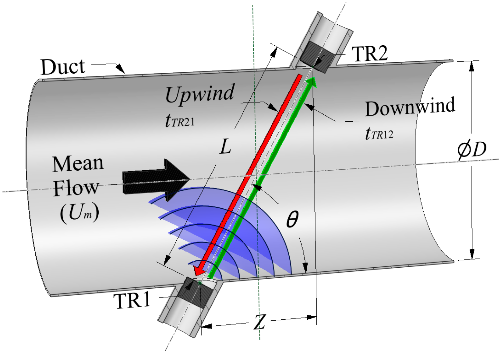
2. Theory
3. Design
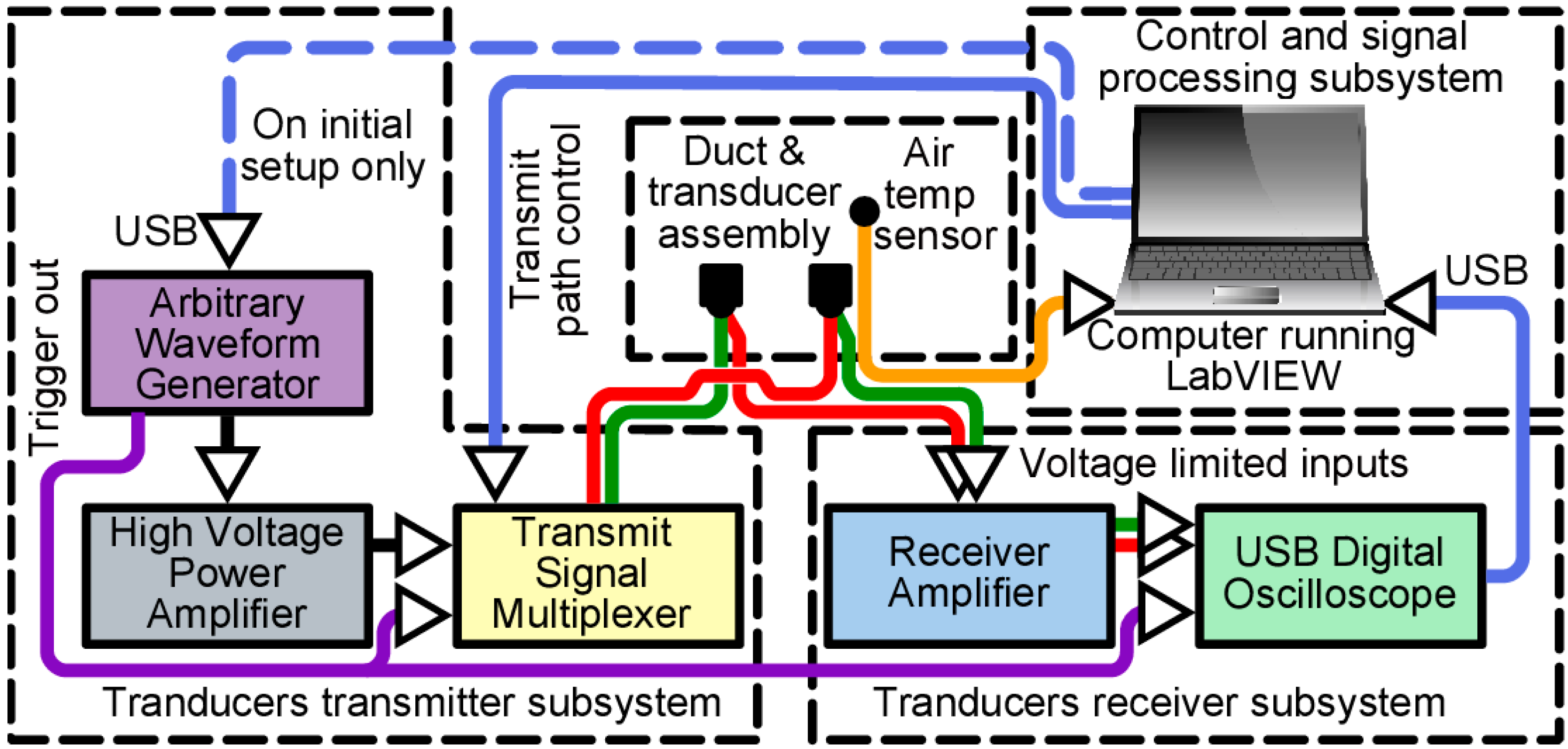
3.1. HVAC Ultrasonic Duct Airflow Measurement Development System
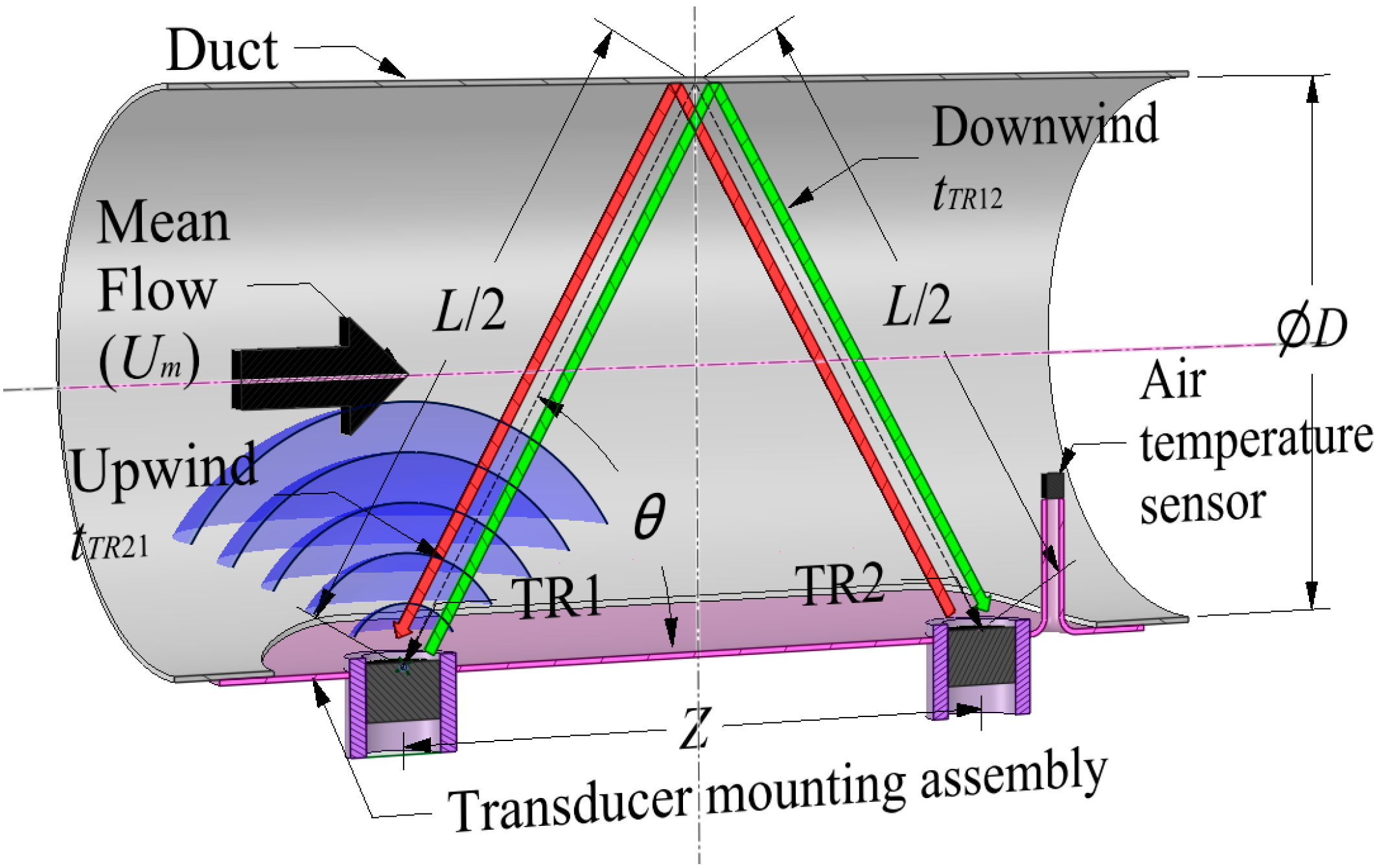
3.2. Transducer Configuration


| Deviation in (mm) | −10 | −5 | 0 | 5 | 10 | |
|---|---|---|---|---|---|---|
| Z | Airflow results (m/s) | 11.050 | 10.512 | 10.000 | 9.512 | 9.050 |
| Deviation from 10 m/s as (%) | 10.497 | 5.125 | 0.000 | −4.875 | −9.502 | |
| D, H | Airflow results (m/s) | 9.987 | 9.997 | 10.000 | 9.997 | 9.988 |
| Deviation from 10 m/s as (%) | −0.131 | −0.032 | 0.000 | −0.030 | −0.119 | |
3.3. Ultrasonic Transducer Transmitter Subsystem

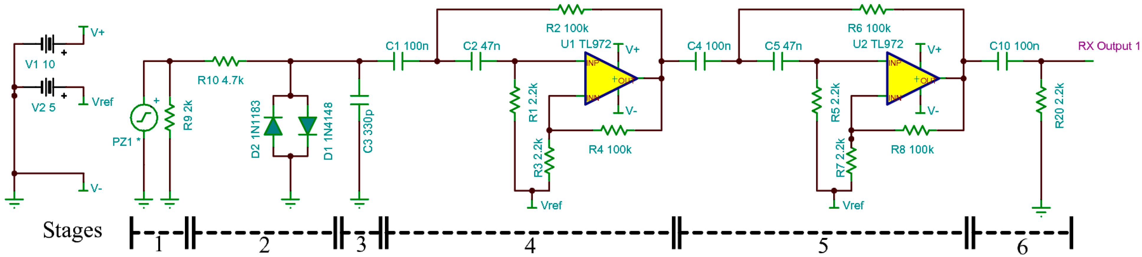
3.4. Ultrasonic Transducer Receiver Subsystem

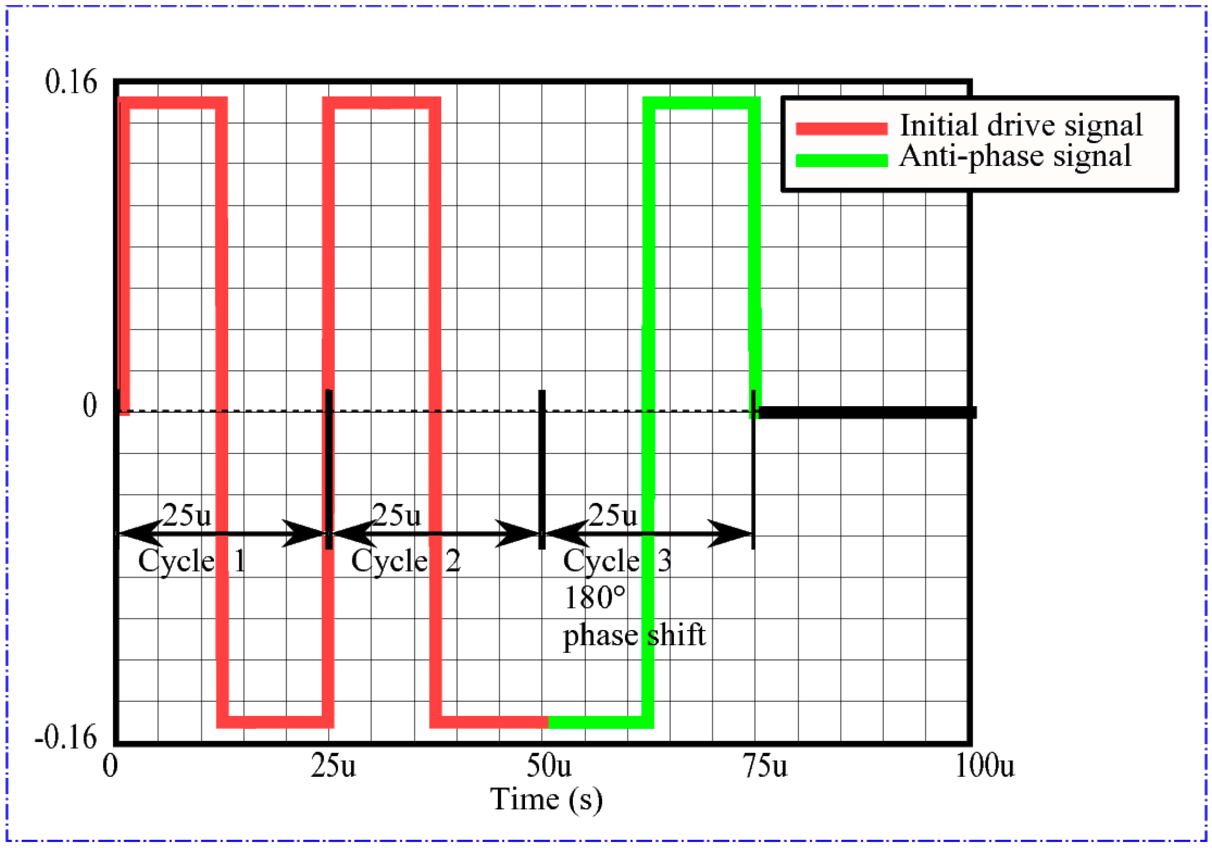
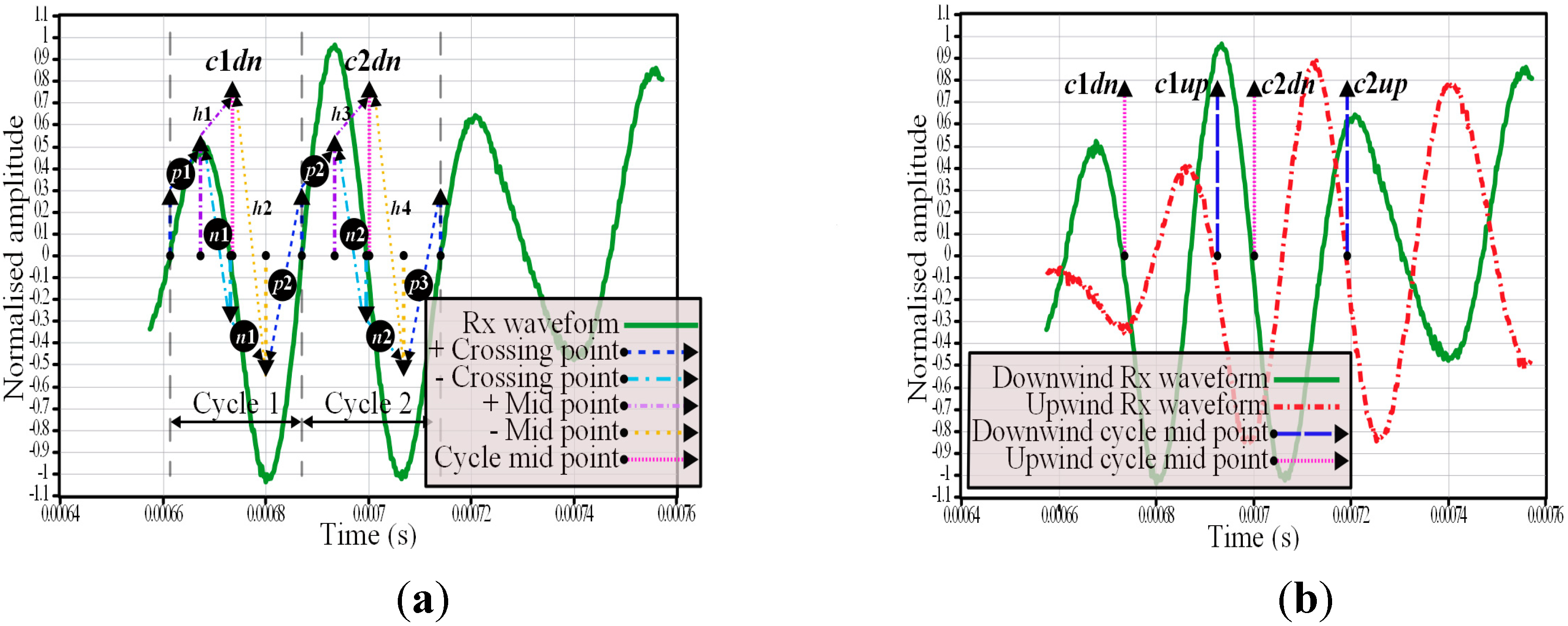
3.5. Signal Processing Method

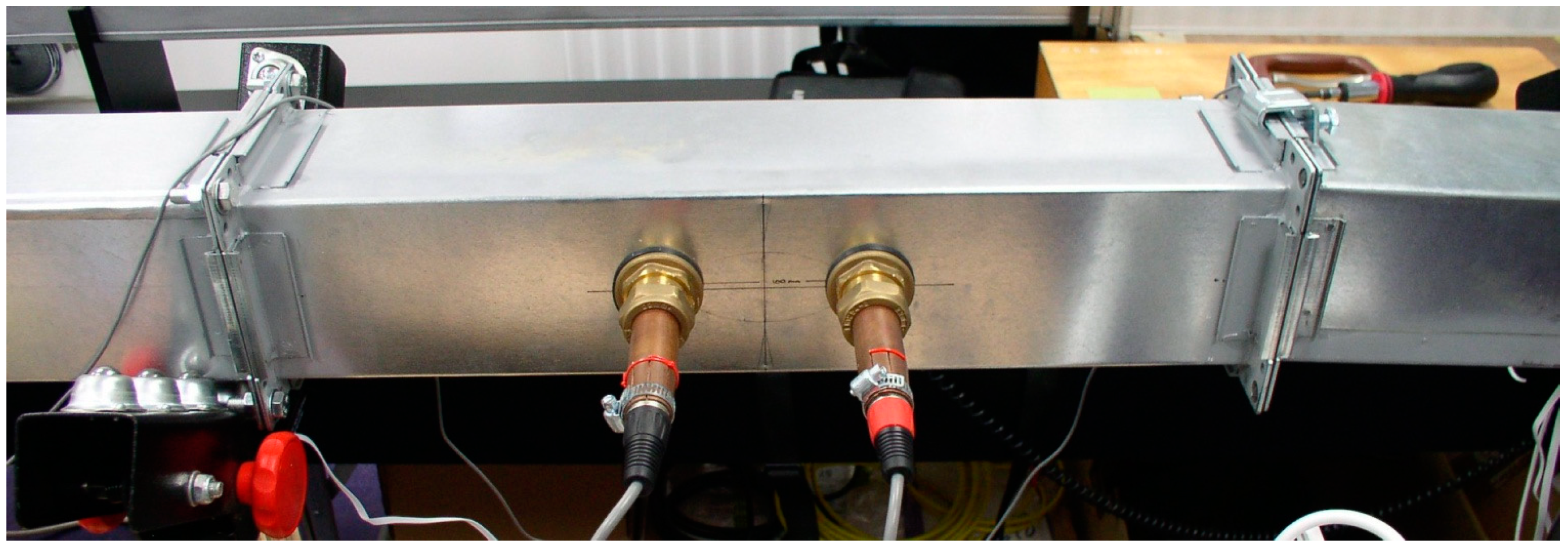
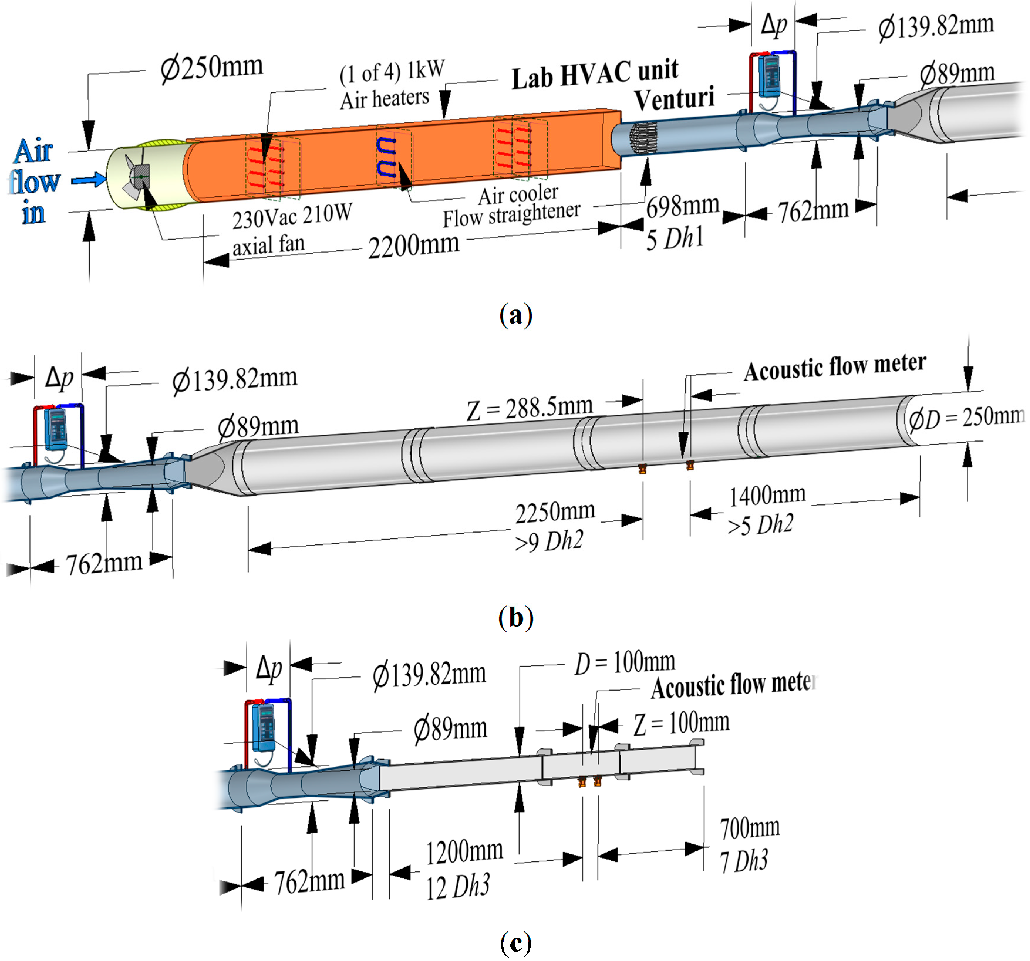
4. Experimental Setup


| Inlet Fan (V) | Mean Venturi Air Temp (°C) | Mean Venturi Δ Pressure Readings (Pa) | Standard Deviation of Venturi Pressure Readings (1 sigma) | Calculated Venturi Mean Mass Flow Rate (kg/m3) | Calculated Venturi Inlet Flow Velocity (m/s) | Calculated Duct Mean Airflow Velocity (m/s) |
|---|---|---|---|---|---|---|
| 120 | 20.9 | 128 | 0.35 | 0.1170 | 6.44 | 2.04 |
| 130 | 20.9 | 156 | 0.63 | 0.1294 | 7.12 | 2.26 |
| 140 | 20.8 | 182 | 0.50 | 0.1397 | 7.68 | 2.44 |
| 150 | 20.7 | 209 | 0.42 | 0.1496 | 8.23 | 2.61 |
| 160 | 20.6 | 231 | 0.43 | 0.1572 | 8.65 | 2.74 |
| 170 | 20.6 | 250 | 0.78 | 0.1634 | 8.99 | 2.85 |
| 180 | 20.6 | 262 | 0.68 | 0.1675 | 9.22 | 2.92 |
| 190 | 20.5 | 275 | 0.40 | 0.1716 | 9.44 | 2.99 |
| 200 | 20.3 | 286 | 0.72 | 0.1748 | 9.61 | 3.04 |
| 210 | 20.2 | 294 | 1.04 | 0.1773 | 9.75 | 3.09 |
| Inlet Fan (V) | Mean Venturi Air Temp (°C) | Mean Venturi Δ Pressure Readings (Pa) | Standard Deviation of Venturi Pressure Readings (1 sigma) | Calculated Venturi Mean Mass Flow Rate (kg/m3) | Calculated Venturi Inlet Flow Velocity (m/s) | Calculated Duct Mean Airflow Velocity (m/s) |
|---|---|---|---|---|---|---|
| 120 | 23.1 | 83 | 0.43 | 0.0941 | 5.21 | 7.99 |
| 130 | 23.2 | 102 | 0.29 | 0.1042 | 5.77 | 8.85 |
| 140 | 23.2 | 122 | 0.45 | 0.1140 | 6.31 | 9.68 |
| 150 | 23.2 | 141 | 0.45 | 0.1223 | 6.77 | 10.39 |
| 160 | 23.1 | 154 | 0.00 | 0.1280 | 7.08 | 10.87 |
| 170 | 23.2 | 166 | 0.21 | 0.1328 | 7.35 | 11.28 |
| 180 | 23.2 | 175 | 0.21 | 0.1364 | 7.55 | 11.58 |
| 190 | 23.2 | 183 | 0.00 | 0.1395 | 7.72 | 11.85 |
| 200 | 23.3 | 189 | 0.29 | 0.1417 | 7.84 | 12.04 |
| 210 | 23.2 | 195 | 0.49 | 0.1439 | 7.96 | 12.22 |
5. Results and Discussion


- Extensive testing on a wider variety of duct sizes and duct shapes with a greater range of airflow velocities.
- Computer modelling of the ultrasonic flowmeter to evaluate its accuracy when it is fitted close to upwind airflow disturbances such as a bend causing duct airflow profile distortion. Test possible solutions to improve on this accuracy, to reduce the amount of expensive laboratory testing needed.
- Experimental testing of the device when fitted in close proximity to disturbances such as bends in different types of duct shape and with turning vanes, where appropriate, and corroborate the computer modelling.
- Extending the function of the device to measure temperature and humidity so that energy efficiency of output can be measured.
- Extending the measurement range of the phase measurement beyond ±180° by using a waveform coarse correlation technique.
- Add corrections required for inaccuracies caused by duct airflow profile.
- Add corrections for humidity change which slightly affect the speed of sound.
6. Conclusions/Outlook
Supplementary Materials
Acknowledgments
Author Contributions
List of Symbols
| Symbol | Description | SI Units |
| c | Speed of sound | m/s |
| D | Diameter of duct | m |
| Dh | Hydraulic diameters | m |
| f0 | Transducer centre frequency | Hz |
| H | Height of rectangular duct | m |
| L | Acoustic path length | m |
| t | Air temperature in degrees | ° |
| tU0 | Transit time of acoustic signal in zero flow state | s |
| Um | Mean airflow inlet velocity | m/s |
| UDTTM | Airflow velocity using phase shift or differential transit time method | m/s |
| UTTM | Airflow velocity using transit time method | m/s |
| Uupper | Typical maximum design air velocity speed | m/s |
| Z | Transducer separation distance with reference to duct axis | m |
| Zmax | Maximum transducer axial separation distance for airflow measurement range | m |
| Δtmax | Typical maximum time of flight difference | s |
| ΔtTR | Differential transit time of the contra-propagating acoustic signals | s |
| tTRij | Transit time of the acoustic signals between transducers | s |
| θ | Angle in degrees between acoustic path and the duct wall | ° |
| tn1 | First negative going zero crossing point time, ∴ 2nd is tn2 | s |
| tp1 | First positive going zero crossing point time, ∴ 2nd is tp2 | s |
| tc1dn | First downwind cycle midpoint time, ∴ 2nd is tc2dn | s |
| tc1up | First upwind cycle midpoint time, ∴ 2nd is tc2up | s |
Conflicts of Interest
References
- Yu, D.; Li, H.; Yang, M. A virtual supply airflow rate meter for rooftop air-conditioning units. Build. Environ. 2011, 46, 1292–1302. [Google Scholar] [CrossRef]
- Cui, J.; Wang, S. A model-based online fault detection and diagnosis strategy for centrifugal chiller systems. Int. J. Therm. Sci. 2005, 44, 986–999. [Google Scholar] [CrossRef]
- Dexter, A.; Pakanen, J. Fault detection and diagnosis methods in real buildings. International Energy Agency, Energy Conservation in Buildings and Community Systems, Annex 34: Computer-aided Evaluation of HVAC System Performance. Available online: http://www.ecbcs.org/annexes/annex34.htm (accessed on 12 September 2014).
- Yu, Y.; Woradechjumroen, D.; Yu, D. A review of fault detection and diagnosis methodologies on air-handling units. Energy Build. 2014, 82, 555–562. [Google Scholar] [CrossRef]
- ASHRAE Handbook, 2009, Fundamentals, S-I ed.; American Society of Heating, Refrigerating and Air Conditioning Engineers: Atlanta, GA, USA, 2009.
- Lynnworth, L.C.; Liu, Y. Ultrasonic flowmeters: Half-century progress report, 1955–2005. Ultrasonics 2006, 44, E1371–E1378. [Google Scholar] [CrossRef] [PubMed]
- Swengel, R.C. Fluid Velocity Measuring System. U.S. Patent. 22 May 1956. Available online: http://www.google.com/patents/US2746291 (accessed on 10 April 2015).
- Gas Flow Measuring Devices. Available online: http://www.sick.com/uk/en-uk/home/products/product_portfolio/flow_solutions/Pages/flow_devices.aspx (accessed on 3 May 2014).
- Tauch, M.; Witrisal, K.; Kudlaty, K.; Noehammer, S.; Wiesinger, M. System identification method for Ultrasonic Intake Air Flow Meter for engine test bed applications. In Proceedings of the 2012 IEEE International Instrumentation and Measurement Technology Conference (I2MTC), Graz, Austria, 13–16 May 2012; pp. 544–548.
- Olmos, P. Ultrasonic velocity meter to evaluate the behaviour of a solar chimney. Meas. Sci. Technol. 2004, 15, N49. [Google Scholar] [CrossRef]
- Van Buggenhout, S.; Ozcan, S.E.; Vranken, E.; van Malcot, W.; Berckmans, D. Acoustical ventilation rate sensor concept for naturally ventilated buildings. In ASHRAE Transactions; Proceedings of of the American-Society-of-Heating-Refrigerating-and-Air-Conditioning-Engineers, Long Beach, CA, USA, June 2007; pp. 192–199.
- Bragg, M.I.; Lynnworth, L.C. Internally-nonprotruding one-port ultrasonic flow sensors for air and some other gases. In Proceedings of the International Conference on Control, Coventry, UK, 21–24 March 1994; Volume 2, pp. 1241–1247.
- Rabalais, R.A.; Sims, L. Ultrasonic Flow Measurement: Technology and Applications in Process and Multiple Vent Stream Situations. Available online: https://www.idc-online.com/technical_references/pdfs/instrumentation/Ultrasonic_Flow_Measurement.pdf (accessed on 15 September 2014).
- Strauss, J.; Weinberg, H.; Kopel, Z. Ultrasound Air Velocity Detector for HVAC Ducts and Method Therefor 1996. U.S. Patent. 10 December 1996. Available online: http://www.google.co.uk/patents/US5583301 (accessed on 12 April 2015).
- Olmos, P. Extending the accuracy of ultrasonic level meters. Meas. Sci. Technol. 2002, 13, 598–600. [Google Scholar] [CrossRef]
- Conrad, K.; Lynnworth, L. Fundamentals of Ultrasonic Flow Meters. pp. 53–54. Available online: http://asgmt.com/paper/fundamentals-of-ultrasonic-flow-meters-2002/ (accessed on 12 April 2015).
- Vermeulen, M.J.M.; Drenthen, J.G.; den Hollander, H. Understanding Diagnostic and Expert Systems in Ultrasonic Flow Meters. Available online: http://asgmt.com/paper/understanding-diagnostic-and-expert-systems-in-ultrasonic-flow-meters-2012/ (accessed on 12 March 2015).
- Bohn, D.A. Environmental Effects on the Speed of Sound. J. Audio Eng. Soc. 1988, 36, 223–231. [Google Scholar]
- Han, D.; Kim, S.; Park, S. Two-dimensional ultrasonic anemometer using the directivity angle of an ultrasonic sensor. Microelectron. J. 2008, 39, 1195–1199. [Google Scholar] [CrossRef]
- Hirata, S.; Kurosawa, M.K.; Katagiri, T. Real-time ultrasonic distance measurements for autonomous mobile robots using cross correlation by single-bit signal processing. In Proceedings of the IEEE International Conference on Robotics and Automation, Kobe, Japan, 12–17 May 2009; pp. 3601–3606.
- Hofmann, F. Fundamentals of Ultrasonic-Flow Measurement for Industrial Applications. Available online: http://www.investigacion.frc.utn.edu.ar/sensores/Caudal/HB_ULTRASONIC_e_144.pdf (accessed on 12 September 2014).
- Chen, Q.; Li, W.; Wu, J. Realization of a multipath ultrasonic gas flowmeter based on transit-time technique. Ultrasonics 2014, 54, 285–290. [Google Scholar] [CrossRef] [PubMed]
- De Cicco, G.; Morten, B.; Prudenziati, M.; Taroni, A.; Canali, C. A 250 KHz Piezoelectric Transducer for Operation in Air: Application to Distance and Wind Velocity Measurements. In Proceedings of the 1982 Ultrasonics Symposium, San Diego, CA, USA, 27–29 October 1982; pp. 321–324.
- Quaranta, A.A.; Aprilesi, G.C.; Cicco, G.D.; Taroni, A. A microprocessor based, three axes, ultrasonic anemometer. J. Phys. E: Sci. Instrum. 1985, 18, 384. [Google Scholar] [CrossRef]
- Bentley, J.P. Principles of Measurement Systems, 4th ed.; Pearson/Prentice Hall: Harlow, UK, 2005; pp. 439–443. [Google Scholar]
- Han, D.; Park, S. Measurement range expansion of continuous wave ultrasonic anemometer. Measurement 2011, 44, 1909–1914. [Google Scholar] [CrossRef]
- Lie, I.; Tiponut, V.; Bogdanov, I.; Ionel, S.; Caleanu, C.D. The Development of CPLD-based Ultrasonic Flowmeter. In Proceedings of the 11th WSEAS International Conference on Circuits, Agios Nikolaos, Crete Island, Greece, 23–25 July 2007; pp. 190–193.
- Cai, C.H.; Regtien, P.P.L. Accurate Digital Time-of-Flight Measurement Using Self-Interference. IEEE Trans. Instrum. Meas. 1993, 42, 990–994. [Google Scholar] [CrossRef]
- Ji-De, H.; Chih-Kung, L.; Chau-Shioung, Y.; Wen-Jong, W.; Chih-Ting, L. High-Precision Ultrasonic Ranging System Platform Based on Peak-Detected Self-Interference Technique. IEEE Trans. Instrum. Meas. 2011, 60, 3775–3780. [Google Scholar] [CrossRef]
- Miller, G.L.; Boie, R.A.; Sibilia, M. Active damping of ultrasonic transducers for robotic applications. In Proceedings of the 1984 IEEE International Conference on Robotics and Automation, Atlanta, GA, USA, 13–15 March 1984; pp. 379–384.
- Buess, C.; Pietsch, P.; Guggenbühl, W.; Koller, E.A. Design and Construction of a Pulsed Ultrasonic Air Flowmeter. IEEE Trans. Biomed. Eng. 1986, BME-33, 768–774. [Google Scholar]
- Baker, R.C. Flow Measurement Handbook: Industrial Designs, Operating Principles, Performance, and Applications; Cambridge University Press: Cambridge, UK, 2000; pp. 24–29. [Google Scholar]
- Jung, J.C.; Seong, P.H. Estimation of the flow profile correction factor of a transit-time ultrasonic flow meter for the feedwater flow measurement in a nuclear power plant. IEEE Trans. Nucl. Sci. 2005, 52, 714–718. [Google Scholar] [CrossRef]
© 2015 by the authors; licensee MDPI, Basel, Switzerland. This article is an open access article distributed under the terms and conditions of the Creative Commons Attribution license (http://creativecommons.org/licenses/by/4.0/).
Share and Cite
Raine, A.B.; Aslam, N.; Underwood, C.P.; Danaher, S. Development of an Ultrasonic Airflow Measurement Device for Ducted Air. Sensors 2015, 15, 10705-10722. https://doi.org/10.3390/s150510705
Raine AB, Aslam N, Underwood CP, Danaher S. Development of an Ultrasonic Airflow Measurement Device for Ducted Air. Sensors. 2015; 15(5):10705-10722. https://doi.org/10.3390/s150510705
Chicago/Turabian StyleRaine, Andrew B., Nauman Aslam, Christopher P. Underwood, and Sean Danaher. 2015. "Development of an Ultrasonic Airflow Measurement Device for Ducted Air" Sensors 15, no. 5: 10705-10722. https://doi.org/10.3390/s150510705
APA StyleRaine, A. B., Aslam, N., Underwood, C. P., & Danaher, S. (2015). Development of an Ultrasonic Airflow Measurement Device for Ducted Air. Sensors, 15(5), 10705-10722. https://doi.org/10.3390/s150510705