
Coarse Initial Orbit Determination for a Geostationary Satellite Using Single-Epoch GPS Measurements

Abstract
:1. Introduction
2. Coarse Initial Orbit Determination Algorithm

3. EKF Scheme

| Nonlinear Dynamics Model Nonlinear Measurement Model State and Measurement |
| Time update Predicted state estimation: Linear approximation: Predicted covariance matrix: |
| Measurement update Predicted Measurement: Measurement matrix linearization: Kalman gain computation: State estimation: Updating posteriori covariance matrix: |
| Measurement Dynamics | EKF Dynamics Error | |
|---|---|---|
| Initial epoch time | UTC 00:00:00 1 January 2006 | - |
| Simulation time | 24 h | - |
| Geopotential model | EGM-96 (Degree: 20, Order: 20) | (Degree: 10, Order: 10) |
| Third-body gravity | Sun, Moon (DE405) | - |
| Solar pressure | 4.57 × 10⁻⁶ N/m2 | - |
| Cross-sectional area | 18.941 m2 | 17.046 m2 (10% error) |
| Satellite mass | 1547 kg | - |
| Numerical integration algorithm | Runge-Kutta 68 | - |
| X | −27,828.9136 (km) | - |
| Y | −31,685.02205 (km) | - |
| Z | 3.51107 (km) | - |
| Vx | 2.30981 (km/s) | - |
| Vy | −2.02866 (km/s) | - |
| Vz | −0.00192 (km/s) | - |
4. Simulation and Results
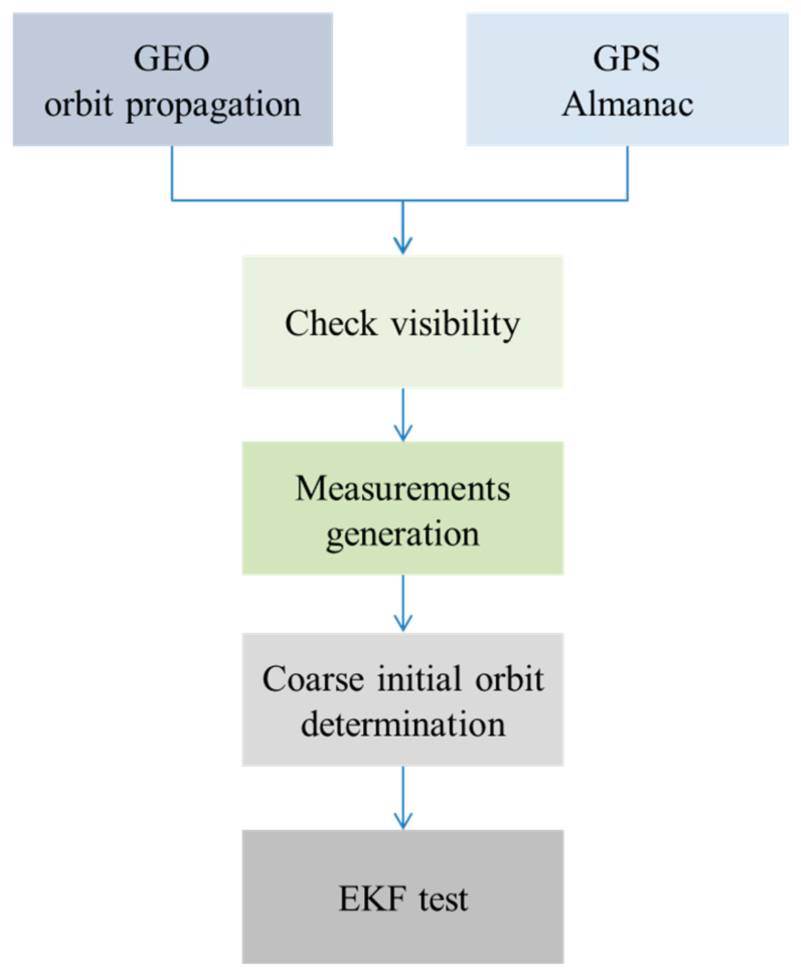
4.1. Simulation Procedure


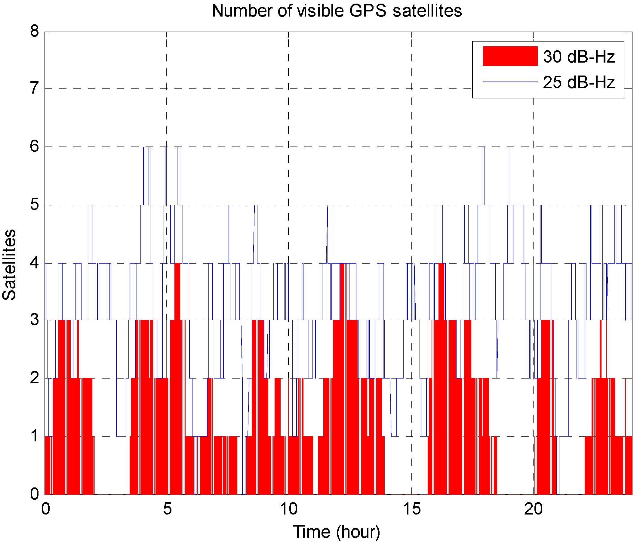
4.2. Generation of Measurements
4.3. Simulation Results
| Point | A | B | C | D |
|---|---|---|---|---|
| UTC time | 00:00:00 | 06:00:00 | 12:00:00 | 18:00:00 |
| x (km) | −27,828.9136 | 31,792.4080 | 27,551.1020 | −32,042.5366 |
| y (km) | −31,685.0220 | −2769.1326 | 31,911.9004 | 27,494.4159 |
| z (km) | 3.5110 | −27.4958 | −5.3747 | 28.3683 |
| vx (km/s) | 2.3098 | 2.0194 | −2.3276 | −1.9989 |
| vy (km/s) | −2.0286 | 2.3185 | 2.0093 | −2.3364 |
| vz (km/s) | −0.0019 | −0.0003 | 0.0019 | 0.0004 |
| Semi-major axis (km) | 42,165.029 | 42,166.897 | 42,165.112 | 42,167.097 |
| Eccentricity | 0.000140 | 0.000108 | 0.000142 | 0.000192 |
| Inclination (deg) | 0.0360 | 0.0378 | 0.0378 | 0.0393 |
| Ascending node (deg) | 56.3009 | 58.8100 | 60.3141 | 61.9844 |
| Argument of perigee (deg) | 348.0949 | 325.9801 | 12.1476 | 17.0192 |
| True anomaly (deg) | 172.4067 | 260.1279 | 348.8802 | 77.4768 |


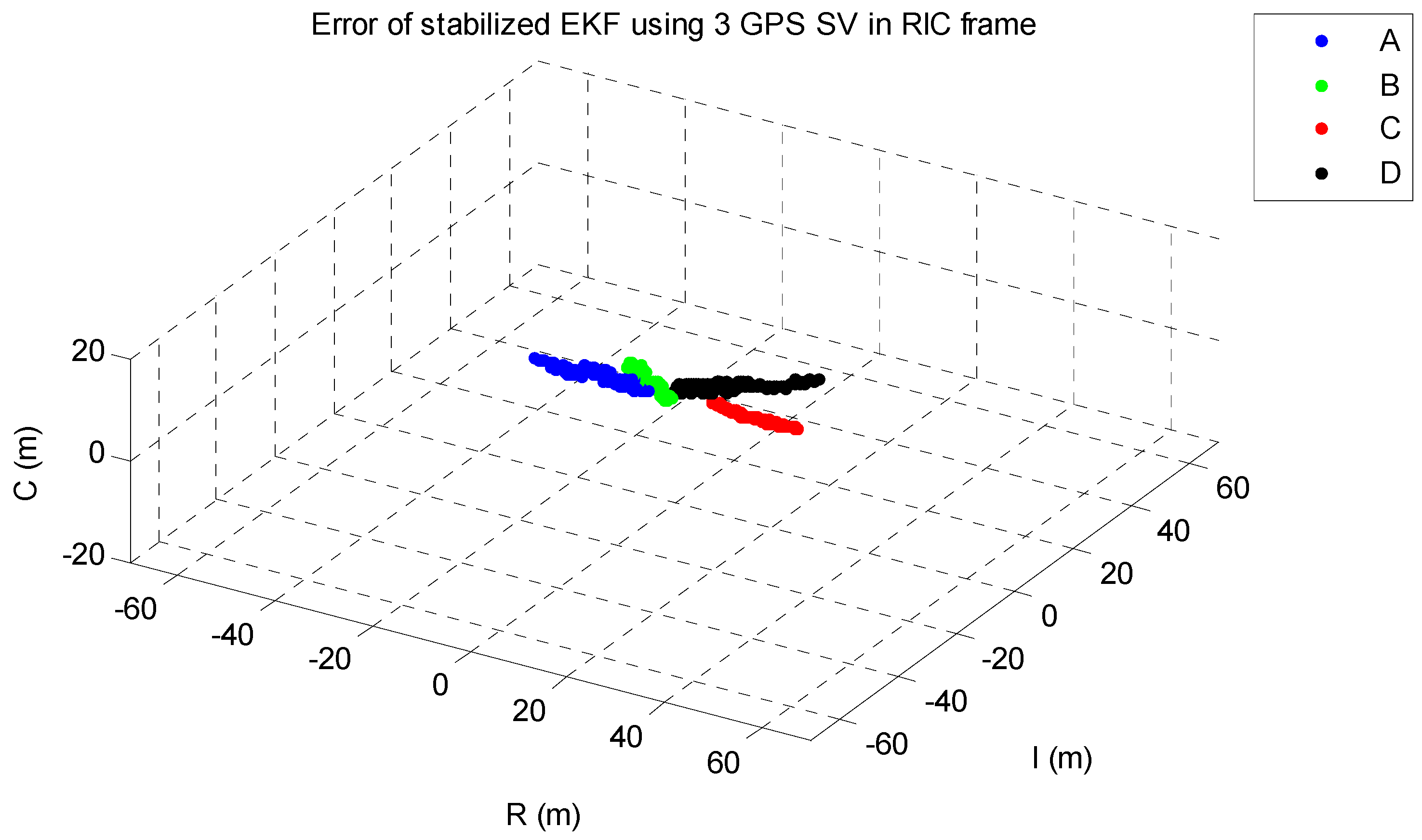
| Residuals | A | B | C | D |
|---|---|---|---|---|
| x (km) | 4.453 | 13.415 | −2.984 | 16.474 |
| y (km) | 5.113 | 16.693 | 8.600 | 20.910 |
| z (km) | −3.511 | 27.495 | 5.374 | −28.268 |
| Vx (km/s) | 0.000325 | −0.000971 | 0.000001 | −0.000963 |
| Vy (km/s) | 0.000331 | 0.000796 | −0.000543 | 0.001067 |
| Vz (km/s) | 0.001920 | 0.000348 | −0.001994 | −0.000458 |
| clock bias (km) | 6.019 | 2.108 | −5.550 | −9.404 |
| clock bias rate (km/s) | 0.000001 | −0.000519 | −0.000276 | 0.000424 |
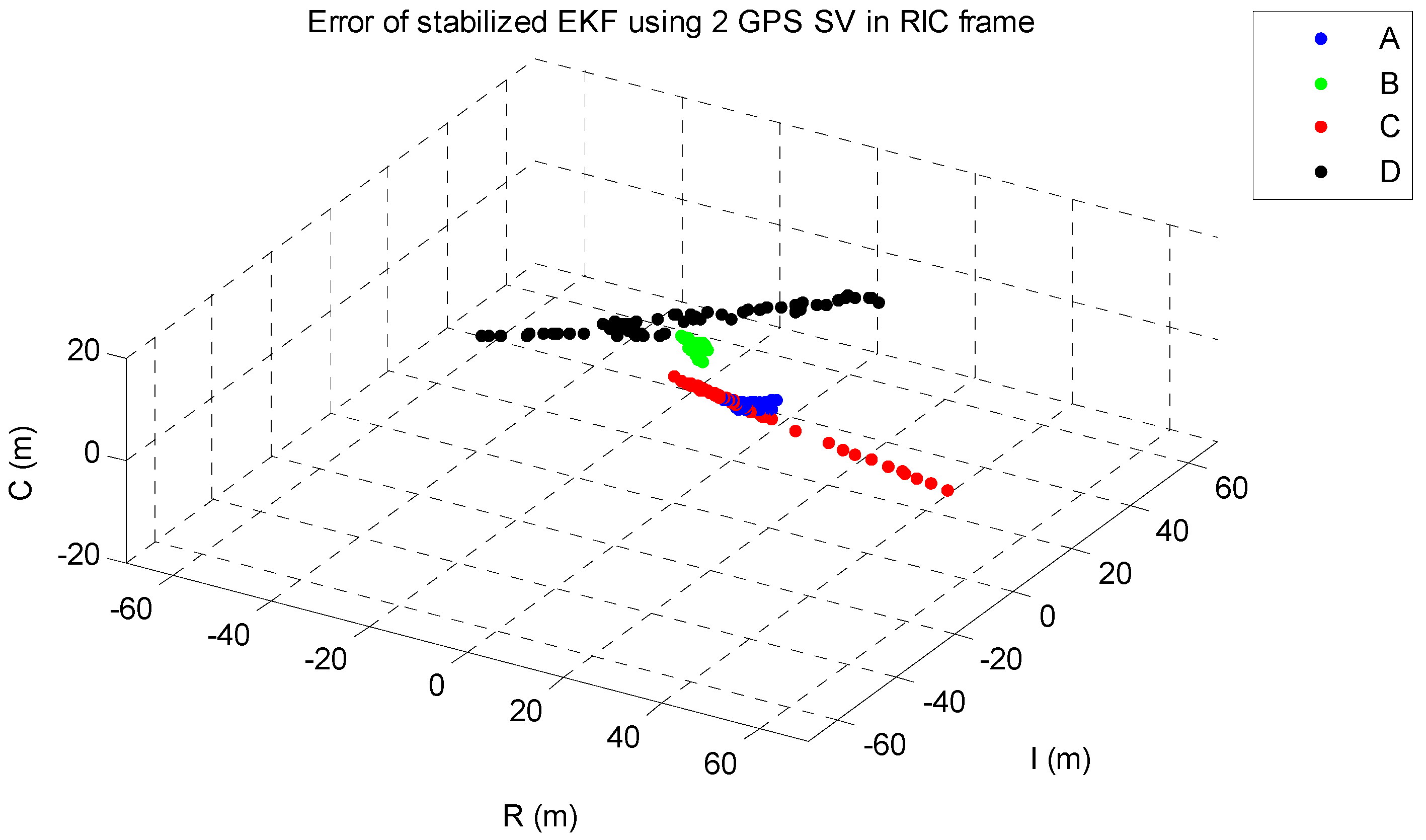
| Residuals | A | B | C | D1 |
|---|---|---|---|---|
| x (km) | 1.908 | 4.642 | 4.951 | 17.425 |
| y (km) | 7.349 | 6.615 | 1.750 | 22.021 |
| z (km) | −3.511 | 27.495 | 5.374 | −28.268 |
| Vx (km/s) | 0.000162 | −0.000236 | 0.000514 | −0.001044 |
| Vy (km/s) | −0.000517 | 0.000156 | 0.000003 | 0.001136 |
| Vz (km/s) | 0.001920 | 0.000348 | −0.001994 | −0.000458 |
| clock bias (km) | 7.156 | −1.598 | −4.319 | −10.088 |
| clock bias rate (km/s) | −0.000194 | −0.000261 | −0.000472 | 0.000194 |
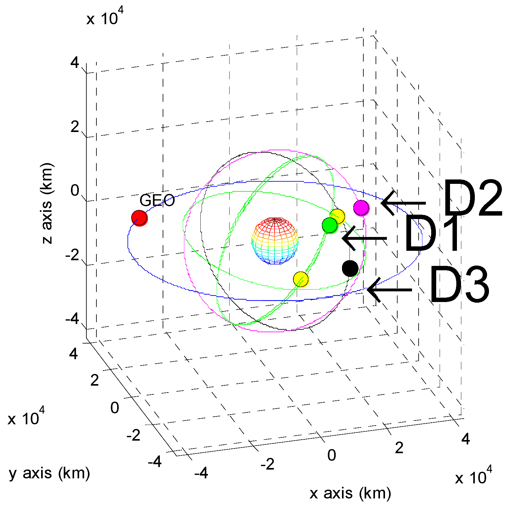
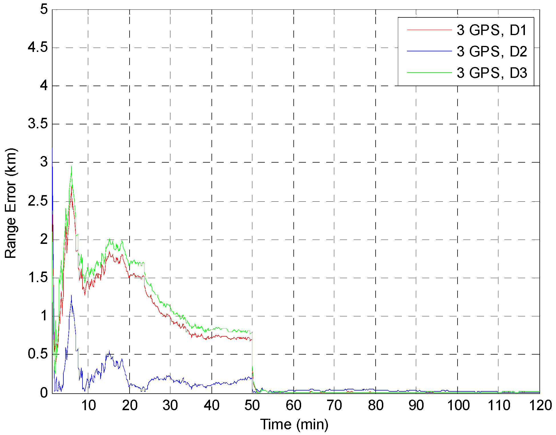
| Residuals | D1 | D2 | D3 |
|---|---|---|---|
| x (km) | 17.425 | 5.2519 | −7.992 |
| y (km) | 22.021 | 7.799 | −7.787 |
| z (km) | −28.268 | −28.268 | −28.268 |
| Vx (km/s) | −0.001044 | −0.000007 | 0.001122 |
| Vy (km/s) | 0.001136 | 0.000249 | −0.000716 |
| Vz (km/s) | −0.000458 | −0.000458 | −0.000458 |
| clock bias (km) | −10.088 | −5.146 | −0.468115 |
| clock bias rate (km/s) | 0.000194 | −0.000050 | −0.000165 |
5. Conclusions
Acknowledgments
Author Contributions
Conflicts of Interest
References
- Choi, J.; Choi, Y.-J.; Yim, H.-S.; Jo, J.H.; Han, W. Two-site optical observation and initial orbit determination for geostationary earth orbit satellites. J. Astron. Space Sci. 2010, 27, 337–343. [Google Scholar] [CrossRef]
- Hwang, Y.; Lee, B.-S.; Kim, H.-Y.; Kim, H.; Kim, J. Orbit determination accuracy improvement for geostationary satellite with single station antenna tracking data. Etri J. 2008, 30, 774–782. [Google Scholar] [CrossRef]
- Moreau, M.C.; Axelrad, P.; Garrison, J.L.; Long, A. GPS receiver architecture and expected performance for autonomous navigation in high earth orbits. Navigation 2000, 47, 191–204. [Google Scholar] [CrossRef]
- Pardal, P.; Kuga, H.; de Moraes, R.V. Robustness assessment between sigma point and extended Kalman filter for orbit determination. J. Aerosp. Eng. 2011, 3, 35. [Google Scholar]
- Vallado, D.A.; McClain, W.D. Fundamentals of Astrodynamics and Applications, 3rd ed.; Springer: NY, USA, 2001. [Google Scholar]
- Zhou, N. Onboard Orbit Determination Using GPS Measurements for Low Earth Orbit Satellites. PhD Thesis, Queensland University of Technology, Brisbane, Austlia, 2004. [Google Scholar]
- Vallado, D.A.; Carter, S.S. Accurate orbit determination from short-arc dense observational data. J. Astronaut. Sci. 1998, 46, 195–213. [Google Scholar]
- Grewal, M.S.; Andrews, A.P. Kalman Filtering: Theory and Practice Using Matlab, 3rd ed.; Wiley: Hoboken, NJ, USA, 2008. [Google Scholar]
- Montenbruck, O.; Gill, E. Satellite Orbits; Springer: Amsterdam, The Netherlands, 2005. [Google Scholar]
- Bolandi, H.; Larki, M.H.A.; Abedi, M.; Esmailzade, M. GPS based onboard orbit determination system providing fault management features for a LEO satellite. J. Navig. 2013, 66, 539–559. [Google Scholar] [CrossRef]
- Vetter, J.R. Fifty years of orbit determination: Development of modern astrodynamics methods. J. Hopkins Appl. Tech. D 2007, 27, 239–252. [Google Scholar]
- Hofmann-Wellenhof, B.; Lichtenegger, H.; Collins, J. GPS Theory and Practice, 5th ed.; Springer-Verlag: New York, NY, USA, 2001. [Google Scholar]
- Chiaradia, A.P.M.; Kuga, H.K.; Prado, A.F.B.D. Onboard and real-time artificial satellite orbit determination using GPS. Math. Probl. Eng. 2013, 2013, 530516:1–530516:8. [Google Scholar] [CrossRef]
- Dong, L. IF GPS Signal Simulator Development and Verification. Master’s Thesis, University of Calgary, AB, Canada, 2003. [Google Scholar]
- Mehlen, C.; Laurichesse, D. In real-time GEO orbit determination using TOPSTAR 3000 GPS receiver. In Proceedings of the ION GPS 2000, Salt Lake City, UT, USA, 19–22 September 2000; pp. 1985–1994.
© 2015 by the authors; licensee MDPI, Basel, Switzerland. This article is an open access article distributed under the terms and conditions of the Creative Commons Attribution license (http://creativecommons.org/licenses/by/4.0/).
Share and Cite
Kim, G.; Kim, C.; Kee, C. Coarse Initial Orbit Determination for a Geostationary Satellite Using Single-Epoch GPS Measurements. Sensors 2015, 15, 7878-7897. https://doi.org/10.3390/s150407878
Kim G, Kim C, Kee C. Coarse Initial Orbit Determination for a Geostationary Satellite Using Single-Epoch GPS Measurements. Sensors. 2015; 15(4):7878-7897. https://doi.org/10.3390/s150407878
Chicago/Turabian StyleKim, Ghangho, Chongwon Kim, and Changdon Kee. 2015. "Coarse Initial Orbit Determination for a Geostationary Satellite Using Single-Epoch GPS Measurements" Sensors 15, no. 4: 7878-7897. https://doi.org/10.3390/s150407878
APA StyleKim, G., Kim, C., & Kee, C. (2015). Coarse Initial Orbit Determination for a Geostationary Satellite Using Single-Epoch GPS Measurements. Sensors, 15(4), 7878-7897. https://doi.org/10.3390/s150407878