
Multi-Layer Sparse Representation for Weighted LBP-Patches Based Facial Expression Recognition

Abstract
:1. Introduction
2. Expression Feature Extraction
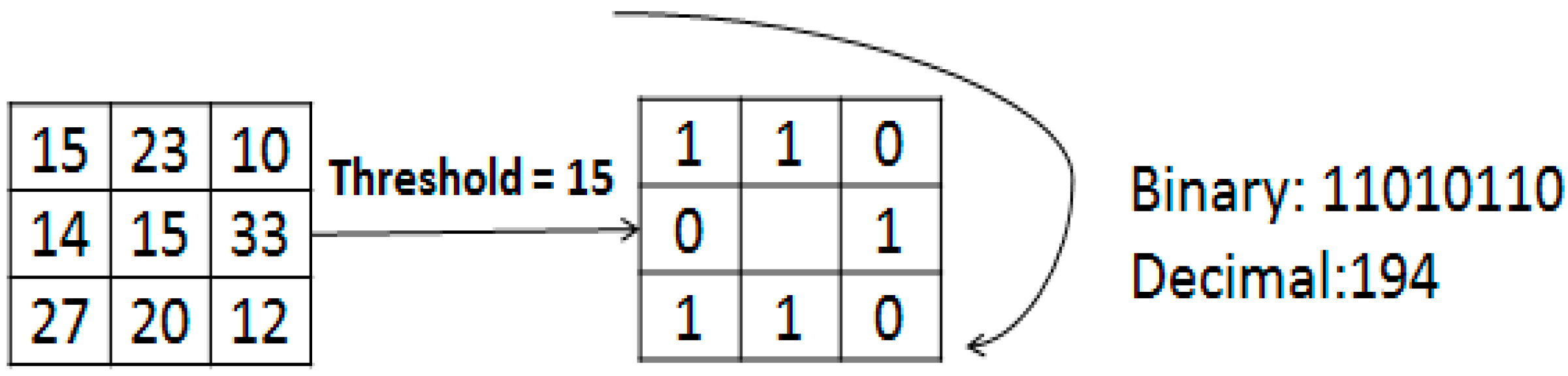
2.1. Local Binary Patterns (LBP)
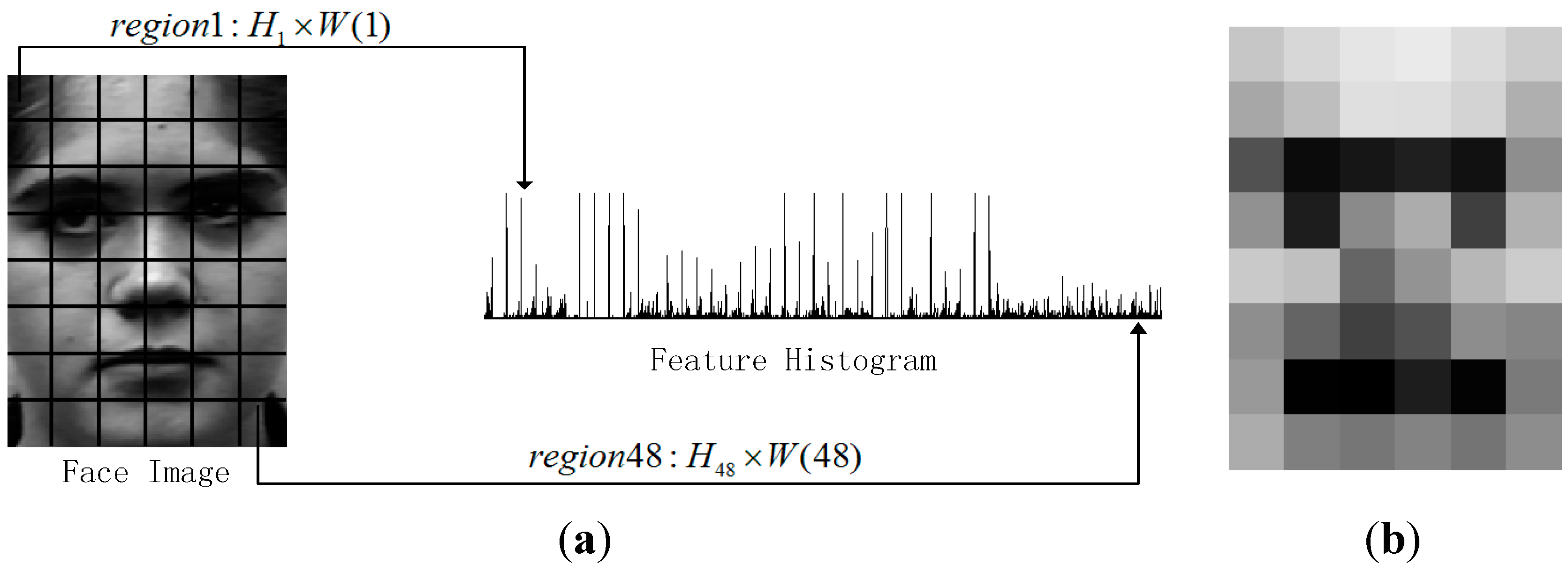
2.2. Weighted Patches
3. Facial Expression Recognition Based on Sparse Representation
| Algorithm 1. Facial Expression Recognition based on Sparse Representation |
| Input: a matrix of training images for C expression classes, a linear feature transform , a test image , and an error tolerance . Output: identity (y) = argmin .
|
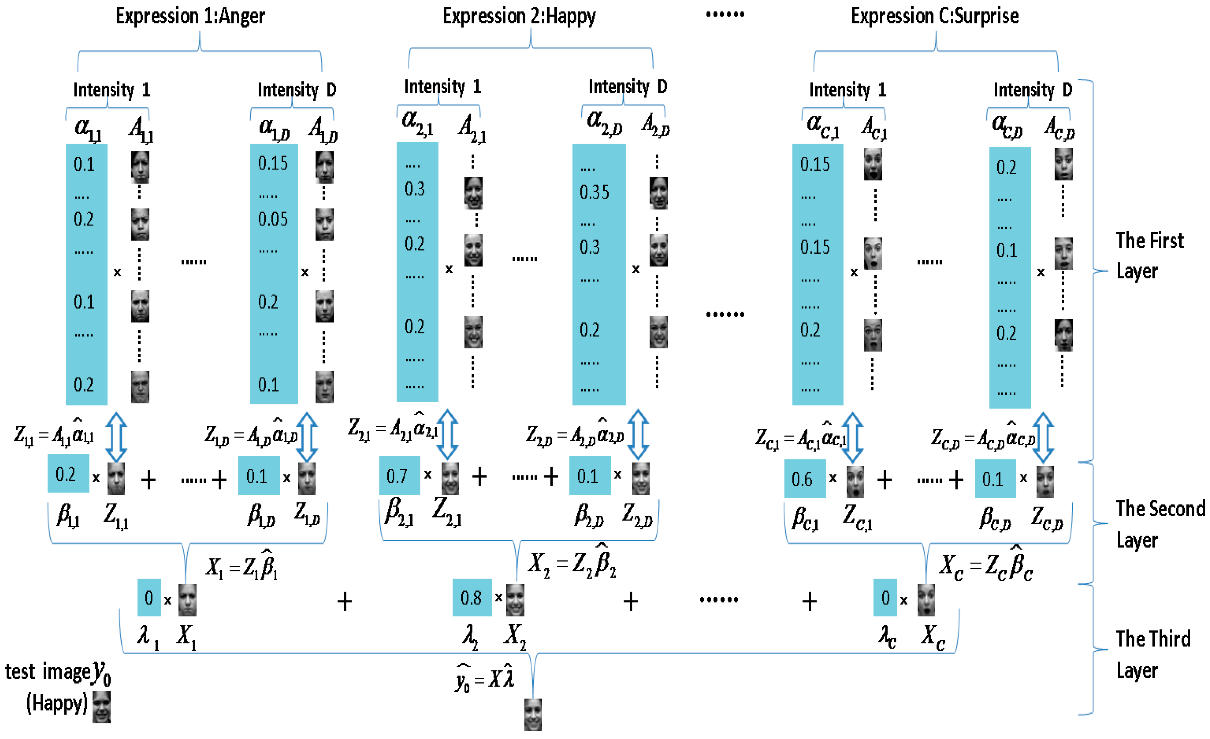
4. Multi-Intensity Facial Expression Recognition Based on Multi-Layer Sparse Representation

| Algorithm 2. Multi-intensity Facial Expression Recognition based on Multi-Layer Sparse Representation |
| Input: training images ; measure matrixes of each layer , , ; A test image , and error tolerance . Output: identity (y) = argmin .
|
5. Experiments
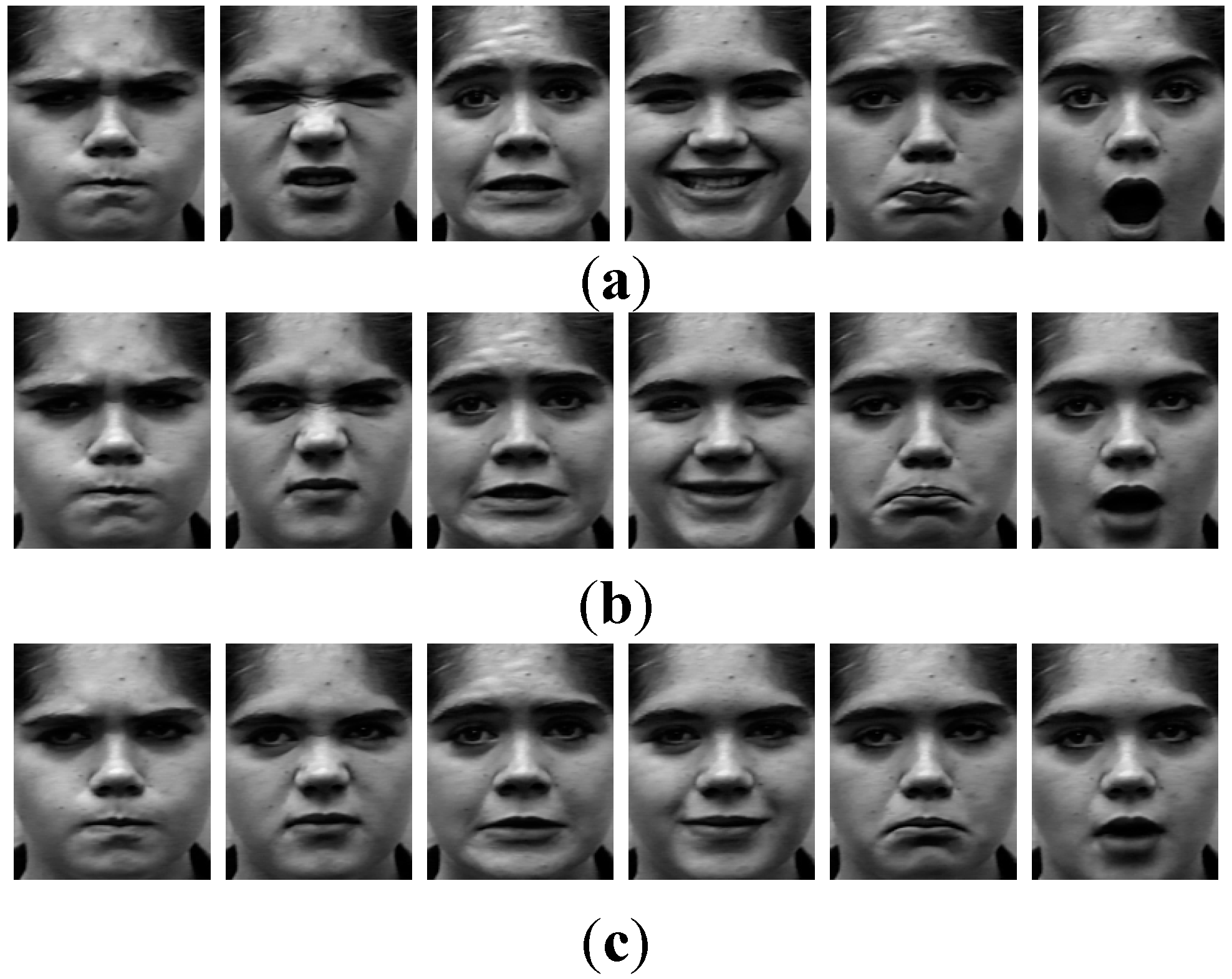
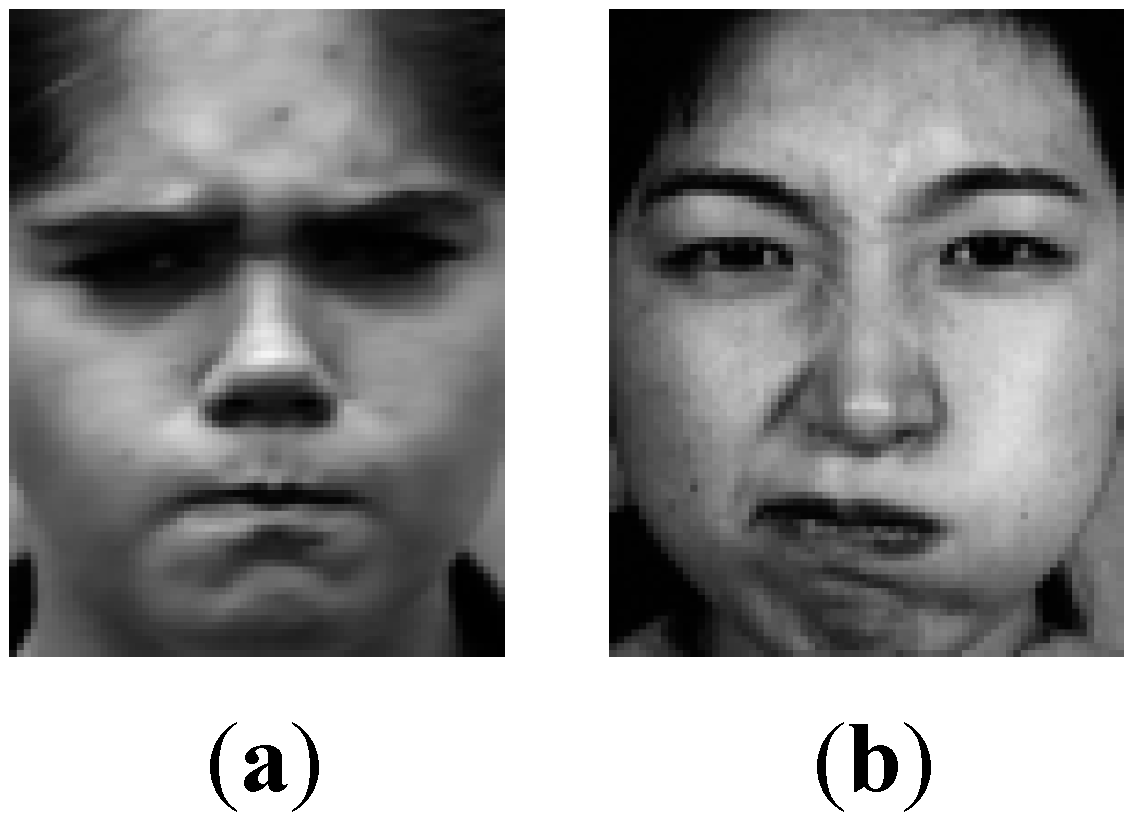
5.1. Data Set
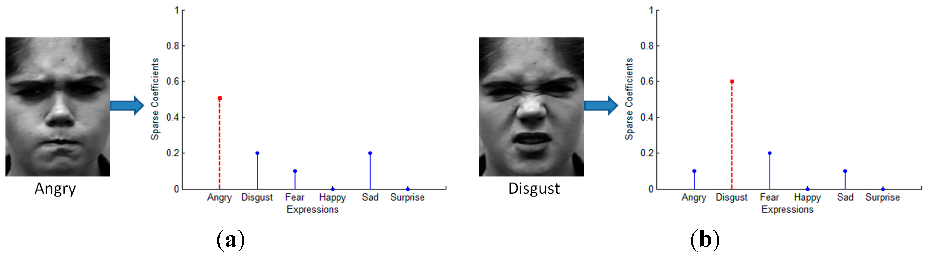
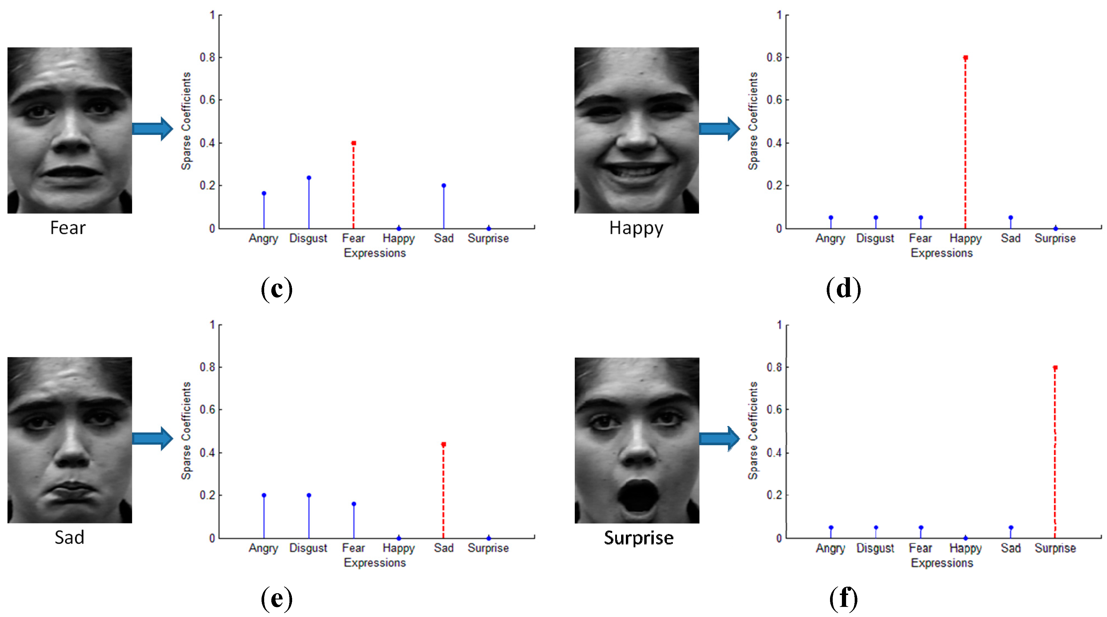
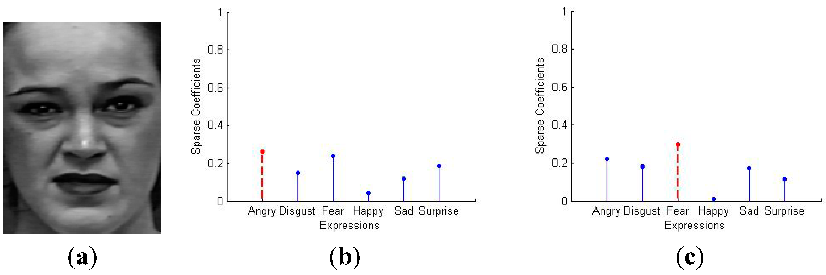
5.2. Sparse Representation for 7-Class Facial Expressions Recognition

| Emotion | Numbers |
|---|---|
| Angry | 45 |
| Disgust | 59 |
| Fear | 25 |
| Happy | 69 |
| Sadness | 28 |
| Surprise | 83 |
| Total | 309 |
| Methods | Recognition Results |
|---|---|
| Sparse Representation (patches without weights) | 85.1% |
| Sparse Representation (patches with weights) | 87% |
| SVM with linear kernel (patches with weights) | 85.4% |
| SVM with RBF kernel (patches with weights) | 86.5% |
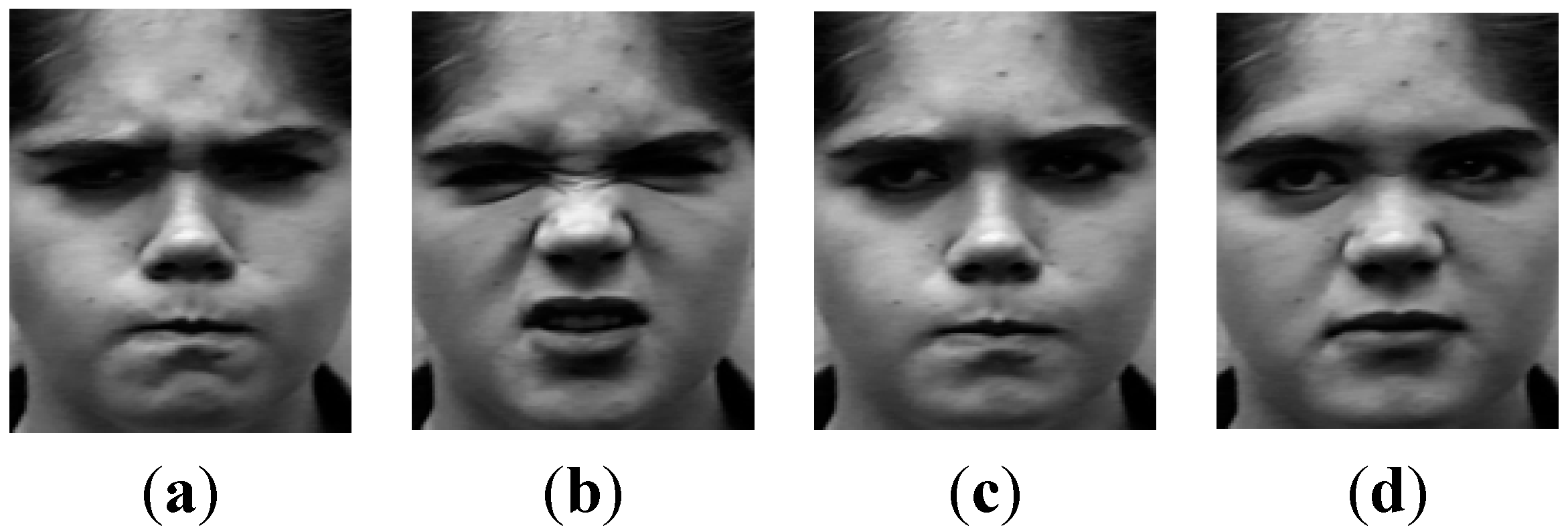
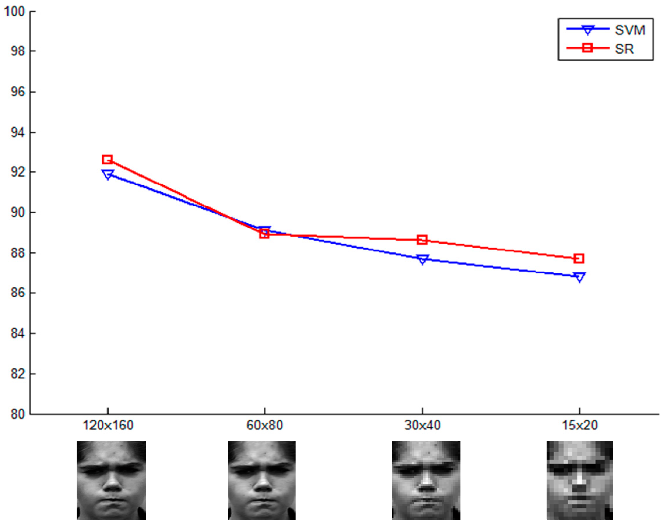
5.3. Data Set Performance over Different Resolutions
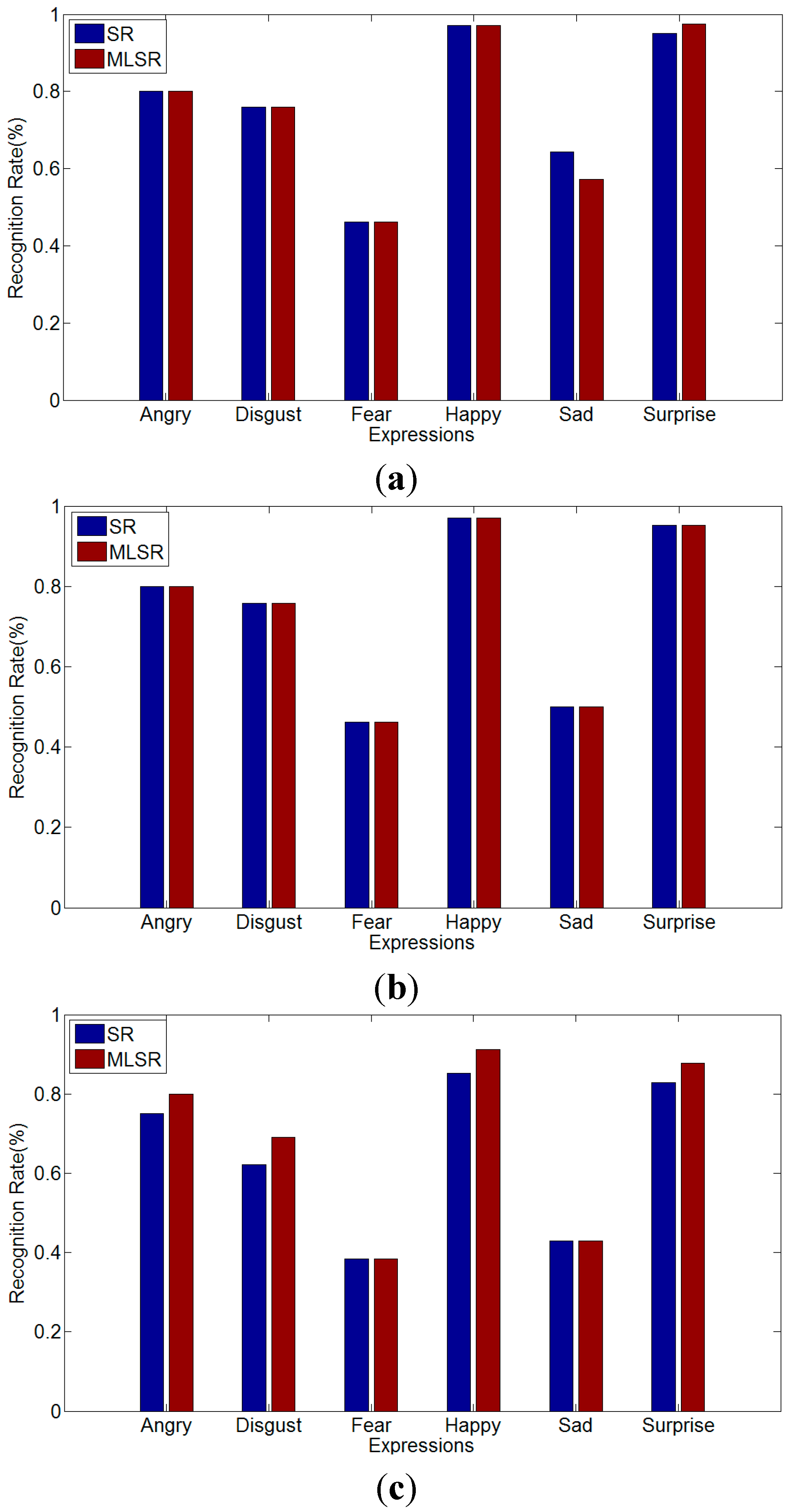
5.4. MLSR for Multi-Intensity Facial Expression Recognition
5.4.1. Recognition Results for Different Intensity


| Methods | High Intensity | Moderate Intensity | Low Intensity |
|---|---|---|---|
| MLSR | 83.56% | 82.26% | 76.35% |
| SVM | 84.07% | 81.43% | 71.96% |
5.4.2. Comparison with State-of-The-Art Performance
| Methods | Subjects | Measure | Recognition Rate |
|---|---|---|---|
| [6] | 97 | 5-fold | 90.90% |
| [7] | 90 | - | 93.66% |
| [10] | 92 | leave-one-subject-out | 94.48% |
| [13] | 97 | 10-fold | 96.26% |
| [14] | 90 | leave-one-subject-out | 96.33% |
| [12] | 96 | 10-fold | 88.4% (92.1%) |
| [11] | 94 | 10-fold | 91.51% |
| [18] | 92 | leave-one-subject-out | 95.17% |
| MLSR | 92 | 10-fold | 92.3% |
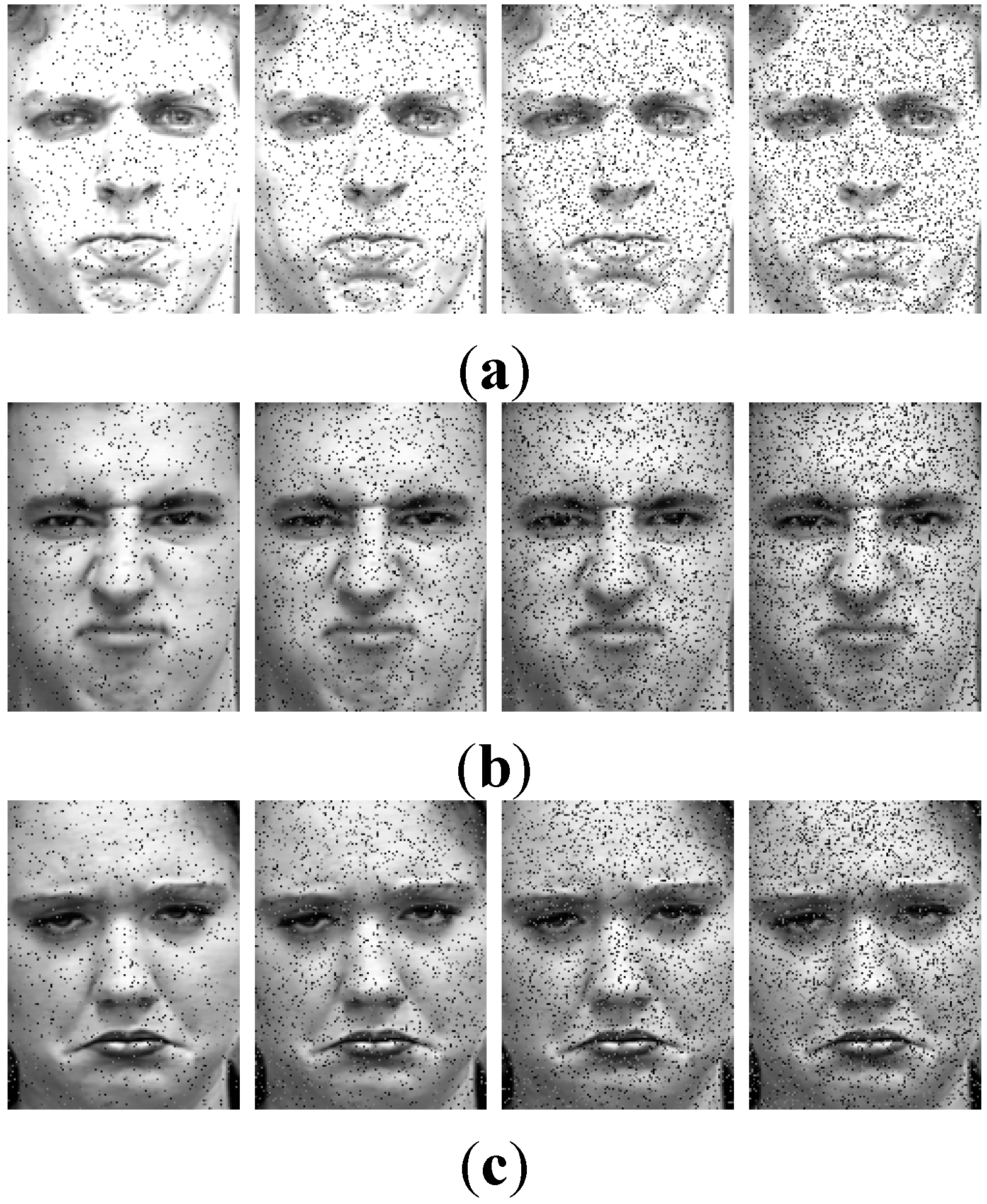
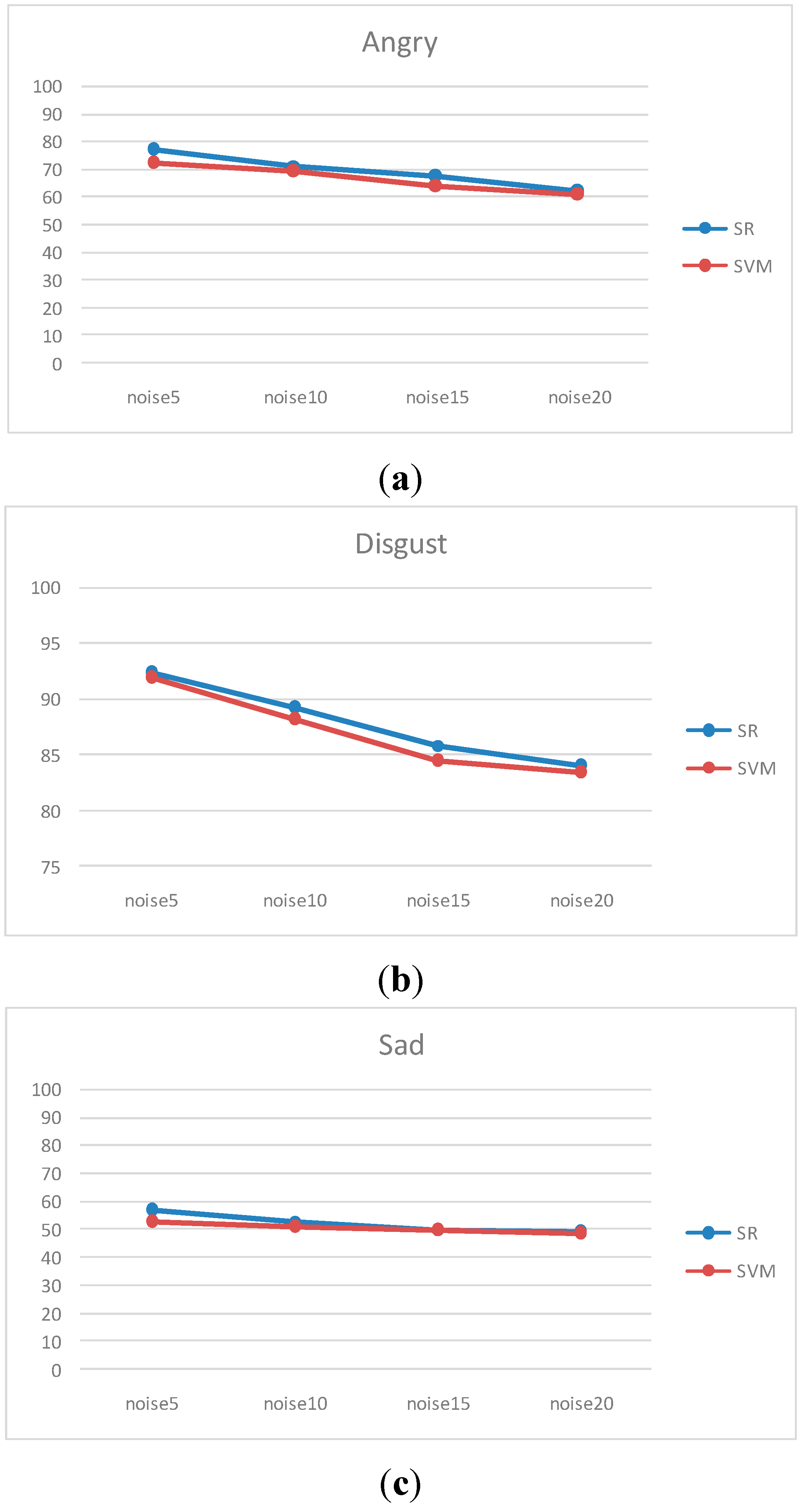
5.5. Performance over Noise

| Expression | Angry | Disgust | Fear | Happy | Neutral | Sad | Surprise | Average | |
|---|---|---|---|---|---|---|---|---|---|
| Noise | |||||||||
| 5 | 77.048 | 92.325 | 68.055 | 94.662 | 78.125 | 56.945 | 92.870 | 83.712 | |
| 10 | 71.238 | 89.231 | 67.499 | 93.015 | 77.438 | 53.055 | 91.144 | 81.559 | |
| 15 | 67.370 | 85.845 | 61.945 | 92.301 | 75.915 | 50.056 | 89.147 | 79.205 | |
| 20 | 61.946 | 83.952 | 56.111 | 91.190 | 73.364 | 49.168 | 87.897 | 76.856 | |
5.6. Cross-Database Experiment
| Methods | SR | SVM |
|---|---|---|
| Train: CK+ Test: JAFFE | 40.5% | 39.4% |
6. Conclusions
Acknowledgments
Author Contributions
Conflicts of Interest
References
- Fang, H.; Mac Parthalain, N.; Aubrey, A.J.; Tam, G.K.L.; Borgo, R.; Rosin, P.L.; Grant, P.W.; Marshall, D.; Chen, M. Facial expression recognition in dynamic sequences: An integrated approach. Pattern Recogn. 2014, 32, 740–748. [Google Scholar]
- Zeng, Z.; Pantic, M.; Roisman, G.; Huang, T. A survey of affect recognition methods: Audio, visual, and spontaneous expressions. IEEE Trans. Pattern Anal. Mach. Intell. 2009, 31, 39–58. [Google Scholar] [CrossRef] [PubMed]
- Sorci, M.; Antonini, G.; Cruz, J.; Robin, T.; Bierlaire, M.; Thiran, J.-P. Modelling human perception of static facial expressions. Image Vis. Comput. 2010, 28, 790–806. [Google Scholar] [CrossRef]
- Tian, Y. Evaluation of face resolution for expression analysis. In Proceedings of the 2004 IEEE Computer Society Conference on Computer Vision and Pattern Recognition Workshops (CVPRW’04), Washington, DC, USA, 27 May–2 June 2004; pp. 82–88.
- Littlewort, G.; Bartlett, M.; Fasel, I.; Susskind, J.; Movellan, J. Dynamics of facial expression extracted automatically from video. Image Vis. Comput. 2006, 24, 615–625. [Google Scholar] [CrossRef]
- Yeasin, M.; Bullot, B.; Sharma, R. From facial expression to level of interest: A spatio-temporal approach. In Proceedings of the 2004 IEEE Computer Society Conference on Computer Vision and Pattern Recognition (CVPR’04), Washington, DC, USA, 27 June–2 July 2004; pp. 922–927.
- Aleksic, P.S.; Katsaggelos, A.K. Automatic facial expression recognition using facial animation parameters and multi-stream HMMS. IEEE Trans. Inf. Foren. Secur. 2006, 1, 3–11. [Google Scholar] [CrossRef]
- Tian, Y.L.; Kanade, T.; Cohn, J. Recognizing action units for facial expression analysis. IEEE Trans. Pattern Anal. Mach. Intell. 2011, 23, 97–115. [Google Scholar] [CrossRef]
- Abdulrahman, M.; Gwadabe, T.R.; Abdu, F.J.; Eleyan, A. Gabor wavelet transform based facial expression recognition using PCA and LBP. In Proceedings of Signal Processing and Communications Applications Conference (SIU), Trabzon, Turkey, 23–25 April 2014; pp. 2265–2268.
- Zhang, L.; Tjondronegoro, D. Facial expression recognition using facial movement features. IEEE Trans. Affect. Comput. 2011, 2, 219–229. [Google Scholar] [CrossRef]
- Gu, W.; Xiang, C.; Venkatesh, Y.V.; Huang, D.; Lin, H. Facial expression recognition using radial encoding of local Gabor features and classifier synthesis. Pattern Recogn. 2012, 45, 80–91. [Google Scholar] [CrossRef]
- Shan, C.; Gong, S.; McOwan, P.W. Robust facial expression recognition using local binary patterns. In Proceedings of the 2005 IEEE International Conference on Image Processing (ICIP’05), Genova, Italy, 11–14 September 2005; pp. 370–373.
- Zhao, G.Y.; Pietikainen, M. Dynamic texture recognition using local binary patterns with an application to facial expressions. IEEE Trans. Pattern Anal. Mach. Intell. 2007, 29, 915–928. [Google Scholar] [CrossRef] [PubMed]
- Li, Z.S.; Imai, J.; Kaneko, M. Facial expression recognition using facial-component-based bag of words and PHOG descriptors. Inf. Med. Technol. 2010, 5, 1003–1009. [Google Scholar]
- Eisenbarth, H.; Alpers, G.W. Happy Mouth and Sad Eyes: Scanning Emotional Facial Expressions. Emotion 2011, 11, 860–865. [Google Scholar] [CrossRef] [PubMed]
- Shan, C.; Gong, S.; McOwan, P.W. Facial expression recognition based on local binary pattern: A comprehensive study. Image Vis. Comput. 2009, 27, 803–816. [Google Scholar] [CrossRef]
- Uçar, A. Facial expression recognition based on significant face components using steerable pyramid transform. In Proceedings of the International Conference on Image Processing, Computer Vision and Pattern Recognition (IPCV’13), Las Vegas, NV, USA, 22–25 July 2013; Volume 2, pp. 687–692.
- Uçar, A.; Demir, Y.; Güzeliş, C. A new facial expression recognition based on curvelet transform and online sequential extreme learning machine initialized with spherical clustering. Neural Comput. Appl. 2014, 1–12. [Google Scholar]
- Donoho, D.L. Compressed sensing. IEEE Trans. Inf. Theor. 2006, 52, 1289–1306. [Google Scholar] [CrossRef]
- Baraniuk, R.G. Compressive sensing. IEEE Signal Process. Mag. 2007, 24, 118–121. [Google Scholar]
- Wright, J.; Yang, Y.; Ganesh, A.; Sastry, S.S.; Ma, Y. Robust face recognition via sparse representation. IEEE Trans. Pattern Anal. Mach. Intell. 2009, 31, 210–227. [Google Scholar] [CrossRef] [PubMed]
- Zhang, S.; Zhao, X.; Lei, B. Robust Facial Expression Recognition via Compressive Sensing. Sensors 2012, 12, 3747–3761. [Google Scholar] [CrossRef] [PubMed]
- Huang, M.; Wang, Z.; Ying, Z. New Method for Facial Expression Recognition Based on Sparse Representation Plus LBP. In Proceedings of the 3rd International Congress on Image and Signal Processing (CISP), Yantai, China, 16–18 October 2010; pp. 1750–1754.
- Liu, P.; Han, S.; Tong, Y. Improving Facial Expression Analysis Using Histograms of Log-Transformed Nonnegative Sparse Representation with a Spatial Pyramid Structure. In Proceedings of the IEEE International Conference and Workshops on Automatic Face and Gesture Recognition (FG), Shanghai, China, 22–26 April 2013; pp. 1–7.
- Ekman, P. Darwin, deception, and facial expression. Ann. N. Y. Acad. Sci. 2003, 1000, 205–221. [Google Scholar] [CrossRef] [PubMed]
- Ou, J.; Bai, X.; Pei, Y.; Ma, L.; Liu, W. Automatic Facial Expression Recognition Using Gabor Filter and Expression Analysis. In Proceedings of the 2010 Second International Conference on Computer Modeling and Simulation, Sanya, China, 22–24 January 2010; pp. 215–218.
- Ouyang, Y.; Sang, N. A Facial Expression Recognition Method by Fusing Multiple Sparse Representation Based Classifiers. In Proceedings of the 10th International Symposium on Neural Networks, Dalian, China, 4–6 July 2013; pp. 479–488.
- Jia, Q.; Liu, Y.; Guo, H.; Luo, Z.X.; Wang, Y.X. Sparse Representation Approach for Local Feature based Expression Recognition. In Proceedings of the International Conference on Multimedia Technology, Hangzhou China, 26–28 July 2011; pp. 4788–4792.
- Ojala, T.; Pietikäinen, M.; Harwood, D. A comparative study of texture measures with classification based on featured distribution. Pattern Recogn. 1996, 29, 51–59. [Google Scholar] [CrossRef]
- Liu, Y.; Wu, F.; Zhang, Z.; Zhuang, Y. Sparse representation using nonnegative curds and whey. In Proceedings of the IEEE Conference on Computer Vision and Pattern Recognition (CVPR), San Francisco, CA, USA, 13–18 June 2010; pp. 3578–3585.
- Ojala, T.; Pietikäinen, M.; Menp, T. Multiresolution grayscale and rotation invariant texture classification with local binary patterns. IEEE Trans. Pattern Anal. Mach. Intell. 2002, 24, 971–987. [Google Scholar] [CrossRef]
- Duda, R.; Hart, P.; Stork, D. Pattern Classification, 2nd ed.; Wiley Interscience: New York, NY, USA, 2000. [Google Scholar]
- Huang, J.; Huang, X.; Metaxas, D. Learning with dynamic group sparsity. In Proceedings of International Conference on Computer Vision, Kyoto, Japan, 29 September–2 October 2009; pp. 64–71.
- Kanade, T.; Cohn, J.F.; Tian, Y. Comprehensive database for facial expression analysis. In Proceedings of the Fourth IEEE International Conference on Automatic Face and Gesture Recognition, Grenoble, France, 28–30 March 2000; pp. 46–53.
- Lucey, P.; Cohn, J.F.; Kanade, T.; Saragih, J.; Ambadar, Z. The Extended Cohn-Kanade Dataset (CK+): A Complete Dataset for Action Unit and Emotion-Specified Expression. In Proceedings of the 3rd IEEE Workshop on CVPR for Human Communication Behavior Analysis, San Francisco, CA, USA, 13–18 June 2010; pp. 94–101.
- Lyons, M.; Akamatsu, S.; Kamachi, M.; Gyoba, J. Coding Facial Expression with Gabor Wavelets. In Proceedings of the 3rd IEEE International Conference on Automatic Face and Gesture Recognition, Nara, Japan, 14–16 April 1988; pp. 200–205.
- SPIDER. Available online: http://www.people.kyb.tuebinggen.mpg.de/spider/index.html (accessed on 20 October 2011).
© 2015 by the authors; licensee MDPI, Basel, Switzerland. This article is an open access article distributed under the terms and conditions of the Creative Commons Attribution license (http://creativecommons.org/licenses/by/4.0/).
Share and Cite
Jia, Q.; Gao, X.; Guo, H.; Luo, Z.; Wang, Y. Multi-Layer Sparse Representation for Weighted LBP-Patches Based Facial Expression Recognition. Sensors 2015, 15, 6719-6739. https://doi.org/10.3390/s150306719
Jia Q, Gao X, Guo H, Luo Z, Wang Y. Multi-Layer Sparse Representation for Weighted LBP-Patches Based Facial Expression Recognition. Sensors. 2015; 15(3):6719-6739. https://doi.org/10.3390/s150306719
Chicago/Turabian StyleJia, Qi, Xinkai Gao, He Guo, Zhongxuan Luo, and Yi Wang. 2015. "Multi-Layer Sparse Representation for Weighted LBP-Patches Based Facial Expression Recognition" Sensors 15, no. 3: 6719-6739. https://doi.org/10.3390/s150306719
APA StyleJia, Q., Gao, X., Guo, H., Luo, Z., & Wang, Y. (2015). Multi-Layer Sparse Representation for Weighted LBP-Patches Based Facial Expression Recognition. Sensors, 15(3), 6719-6739. https://doi.org/10.3390/s150306719