
Sinusoidal Wave Estimation Using Photogrammetry and Short Video Sequences


Abstract
:
1. Introduction
1.1. Contributions
1.2. Related Works
1.2.1. Water as a Diffuse Surface
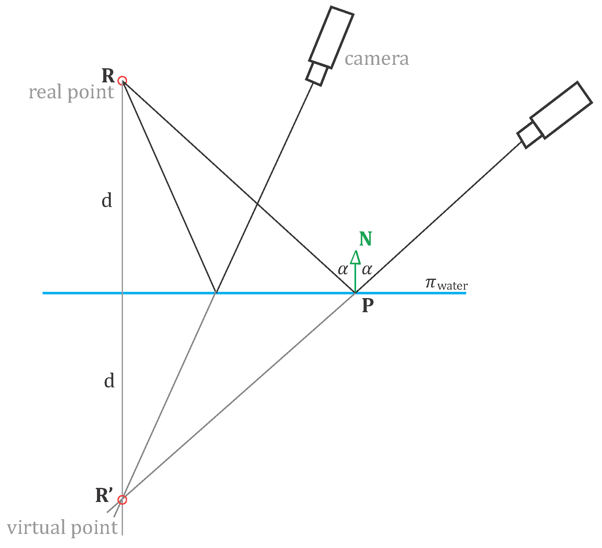
1.2.2. Water as a Specular Surface
1.2.3. Water as a Refractive Medium
2. Preliminaries
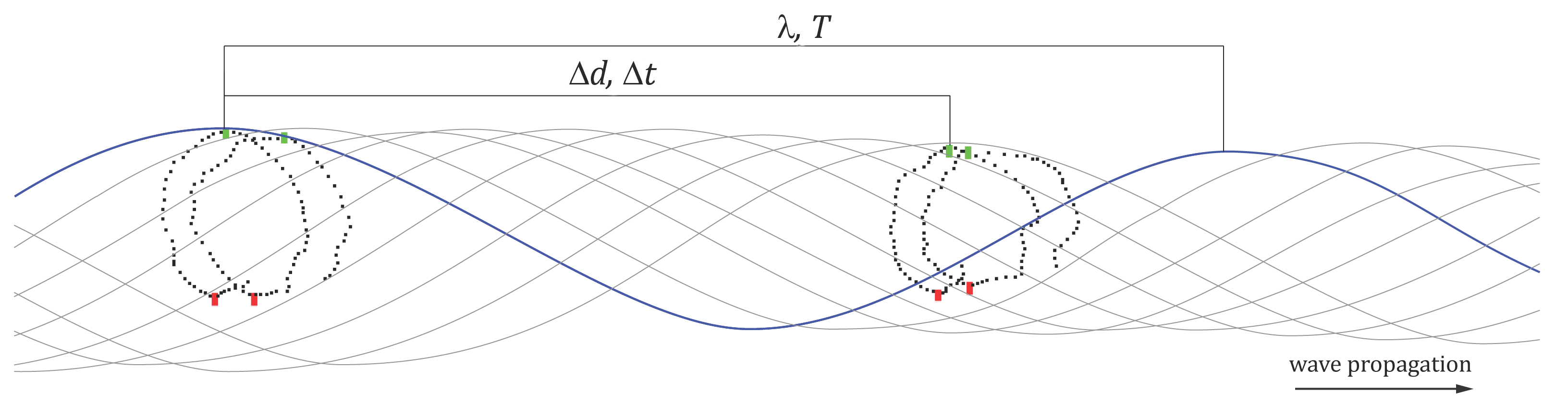
2.1. Derivation of Approximate Wave Parameters
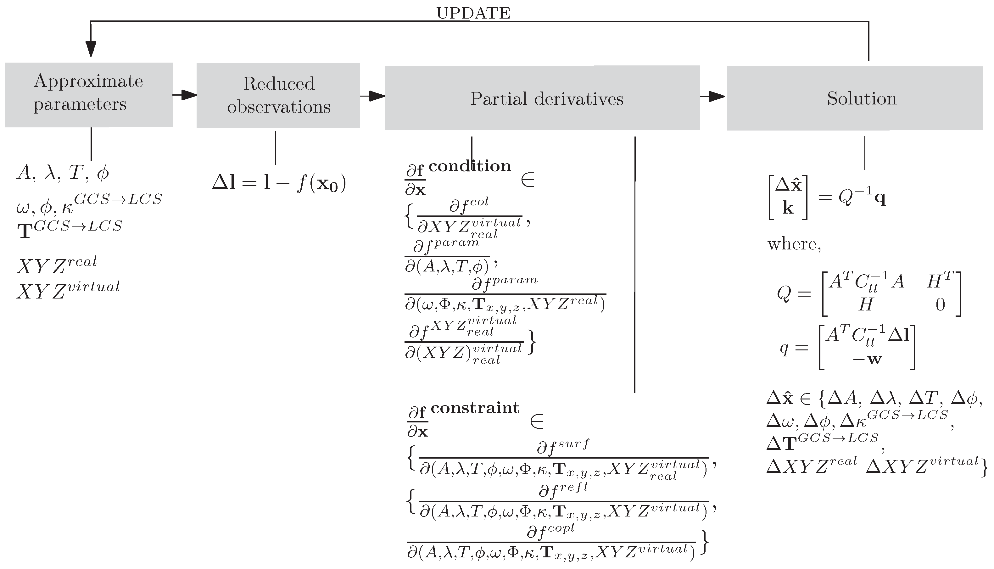
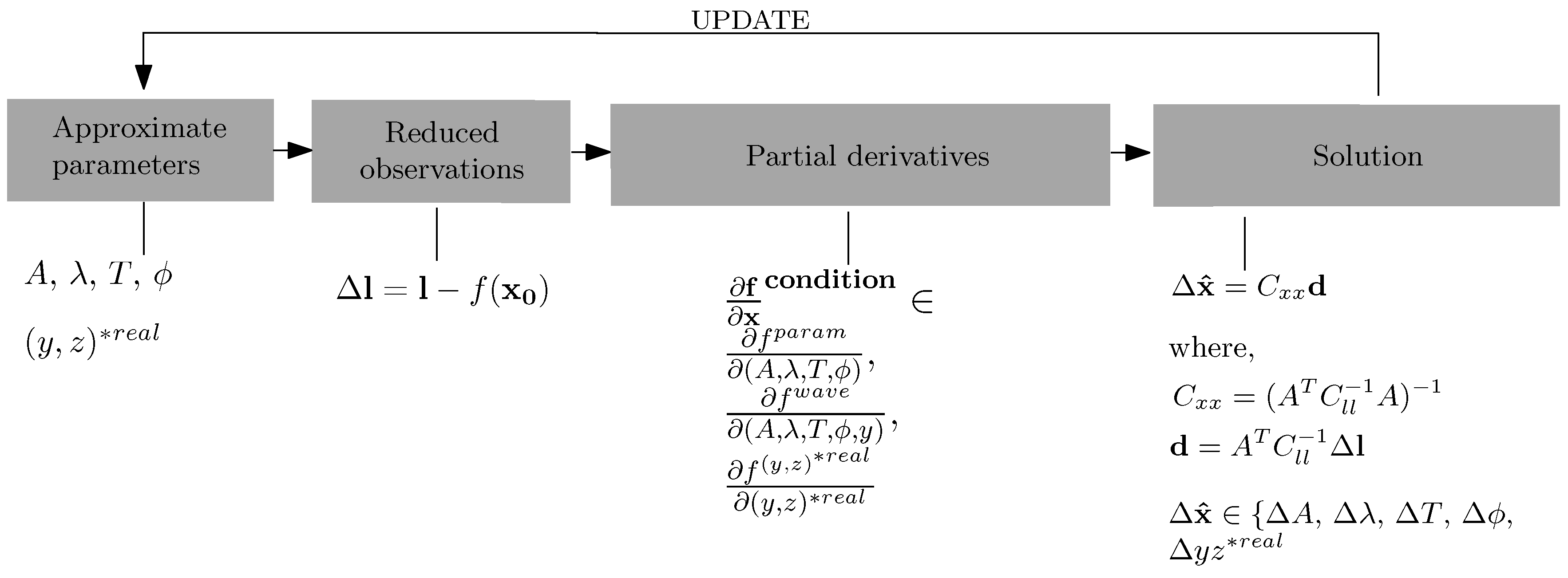
2.2. Optimization Technique
3. Methods
3.1. Water as a Diffuse Surface
3.1.1. Mathematical Model

3.1.2. Image-Based Approximate Wave Retrieval
- clustering of 3D points;
- coupling of neighboring clusters;
- calculation of mean A, T and ϕ from the clusters;
- calculation of mean λ from the couples of clusters.

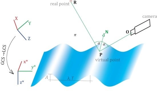
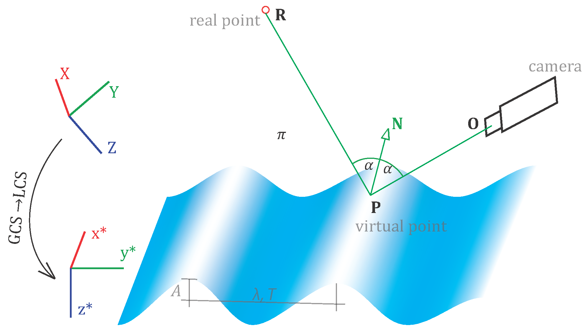
3.2. Water as a Specular Surface

3.2.1. Mathematical Model

- (i)
- ,
- (ii)
- ,
- (iii)
- ,
3.2.2. Derivation of Control Information
- (i)
- roto-translating the global coordinate to a local coordinate system that aligns with the flipping plane,where N = [], λ = , and [] are 3D coordinates of any points lying within the flipping plane.
- (ii)
- performing the actual flipping over the local plane:
- (iii)
- and bringing the point back to the global coordinate system with and .
3.2.3. Derivation of the Approximate Highlight Position
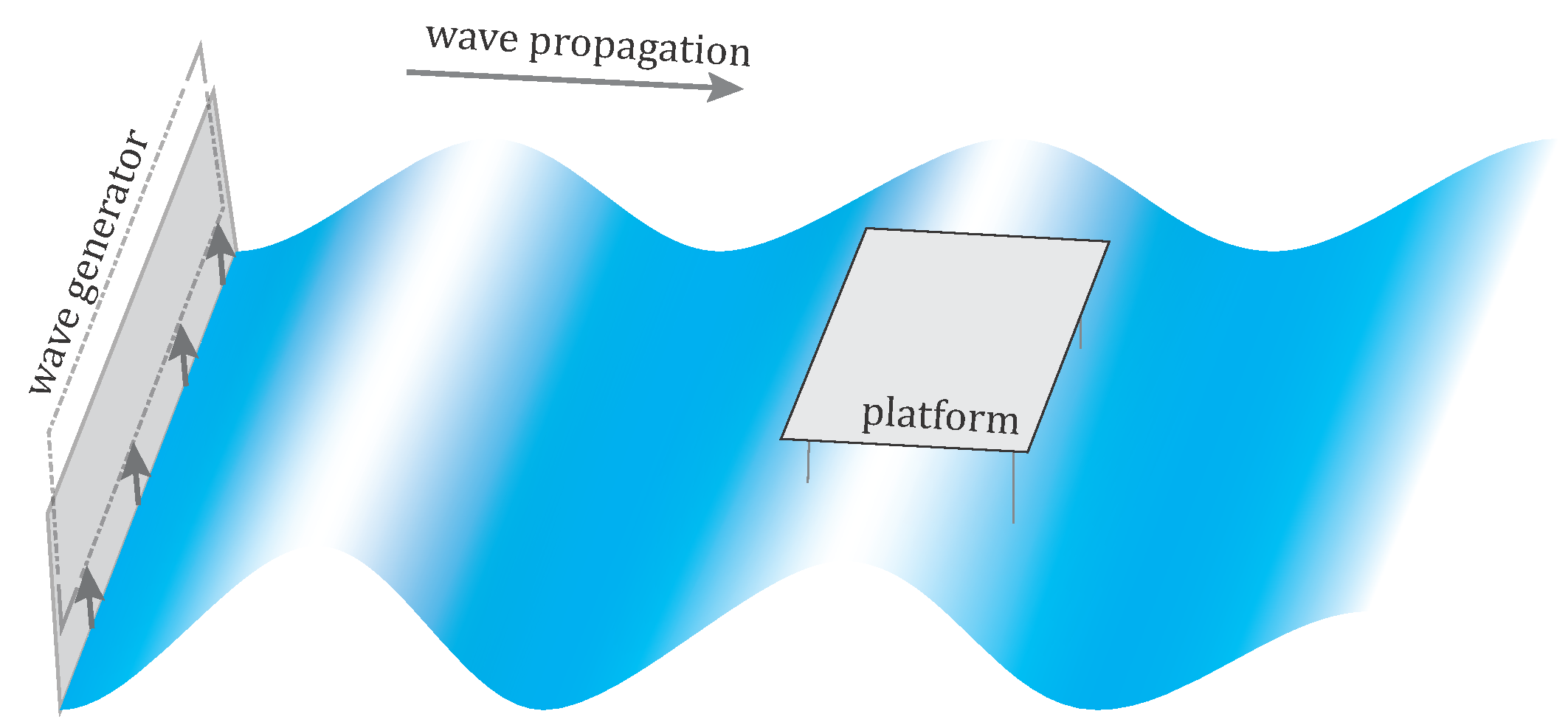
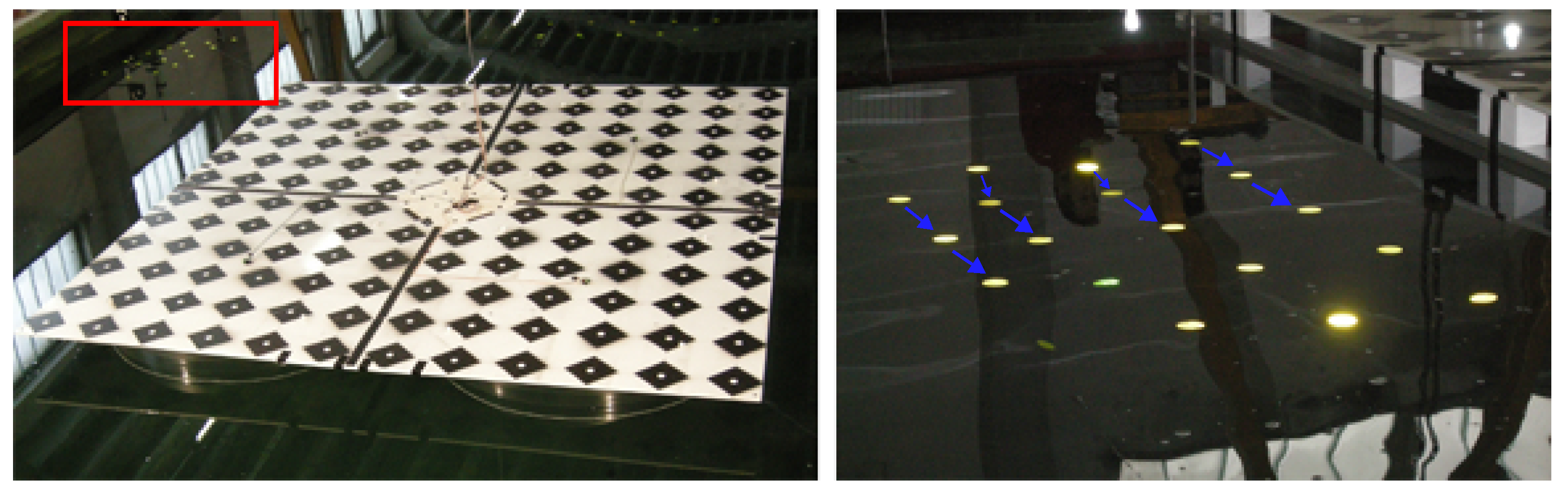
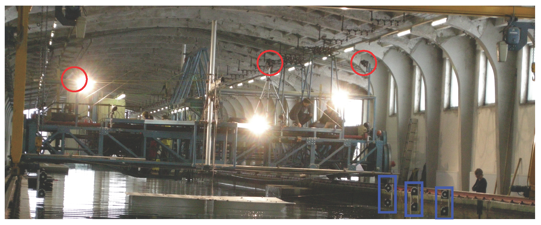
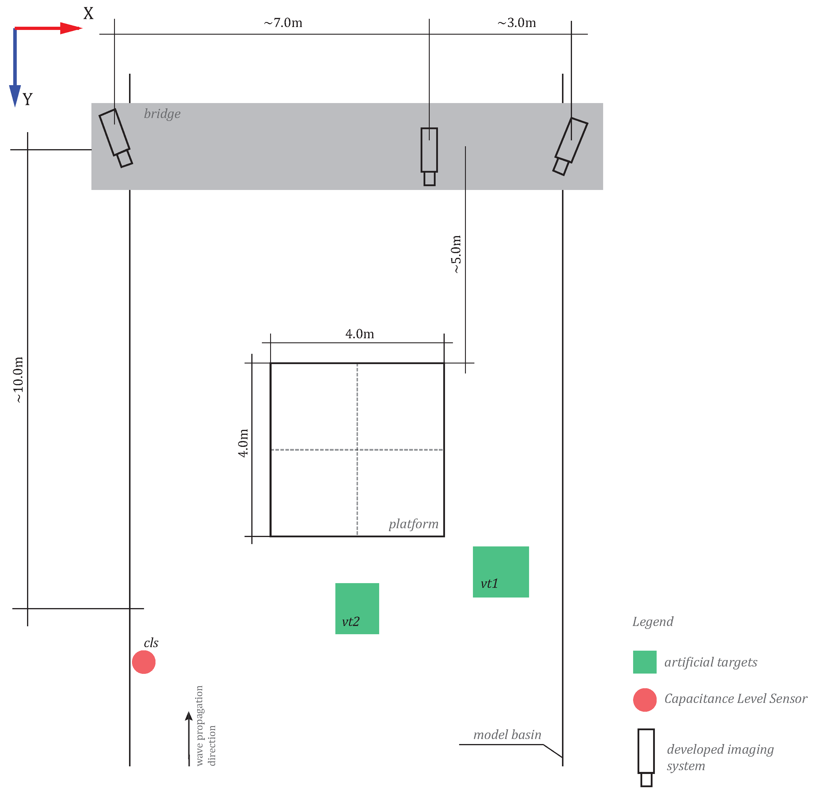
4. Imaging System
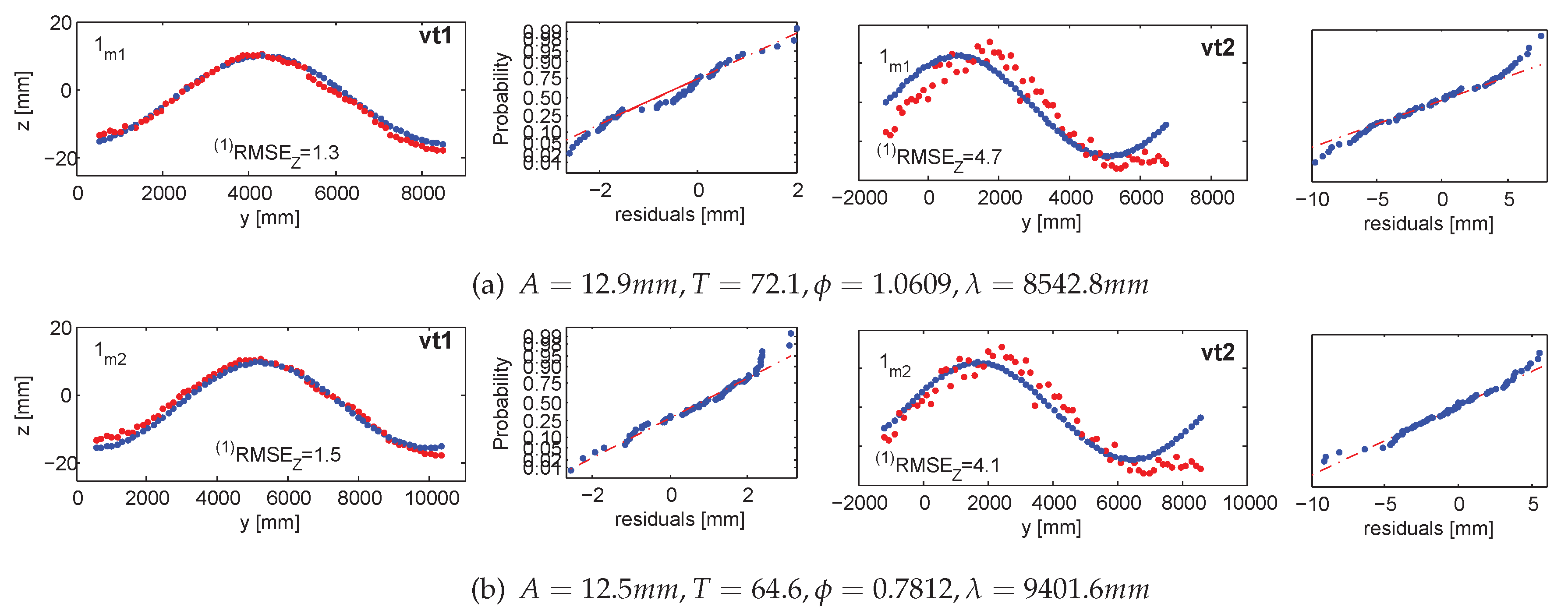
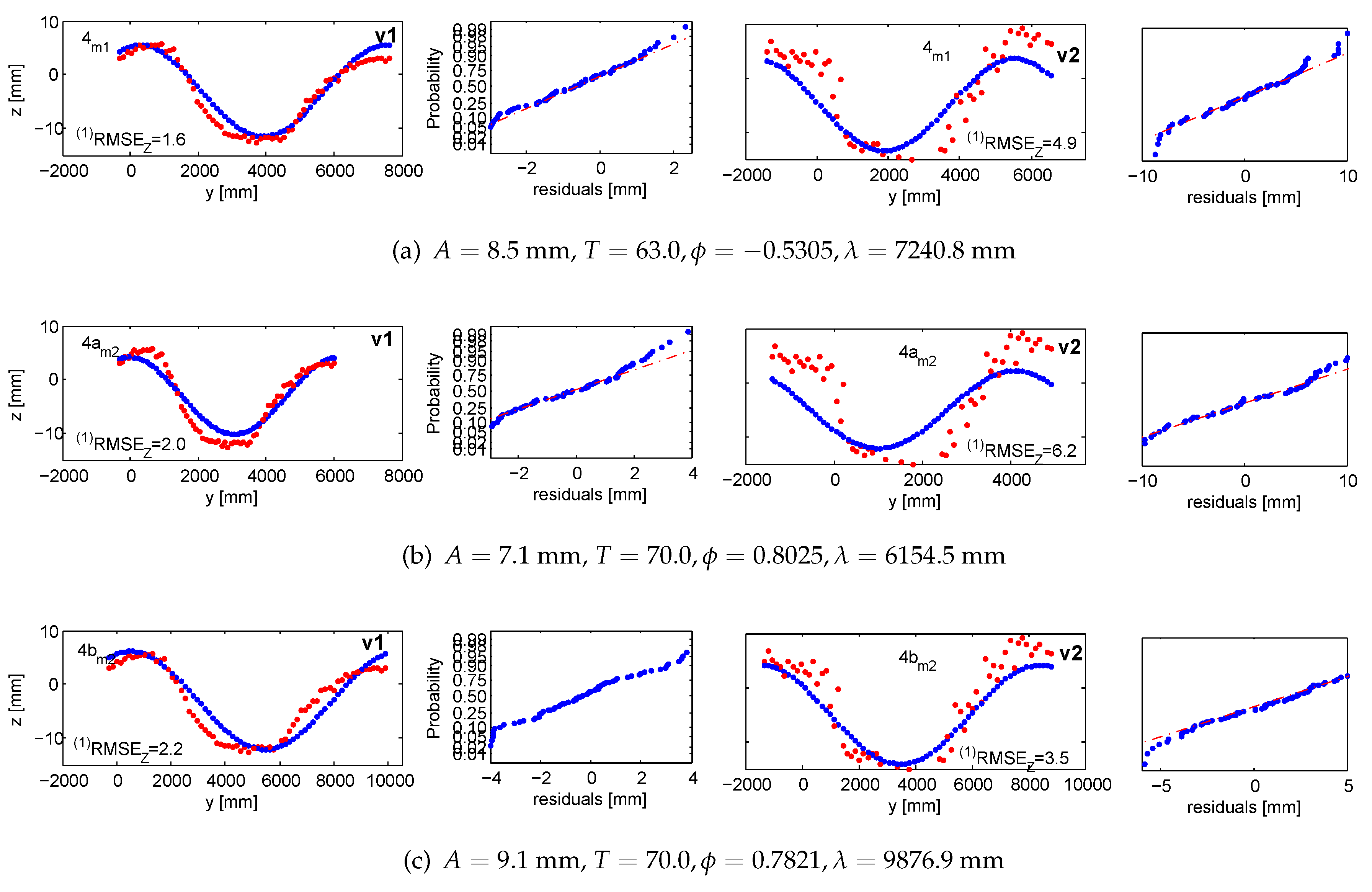
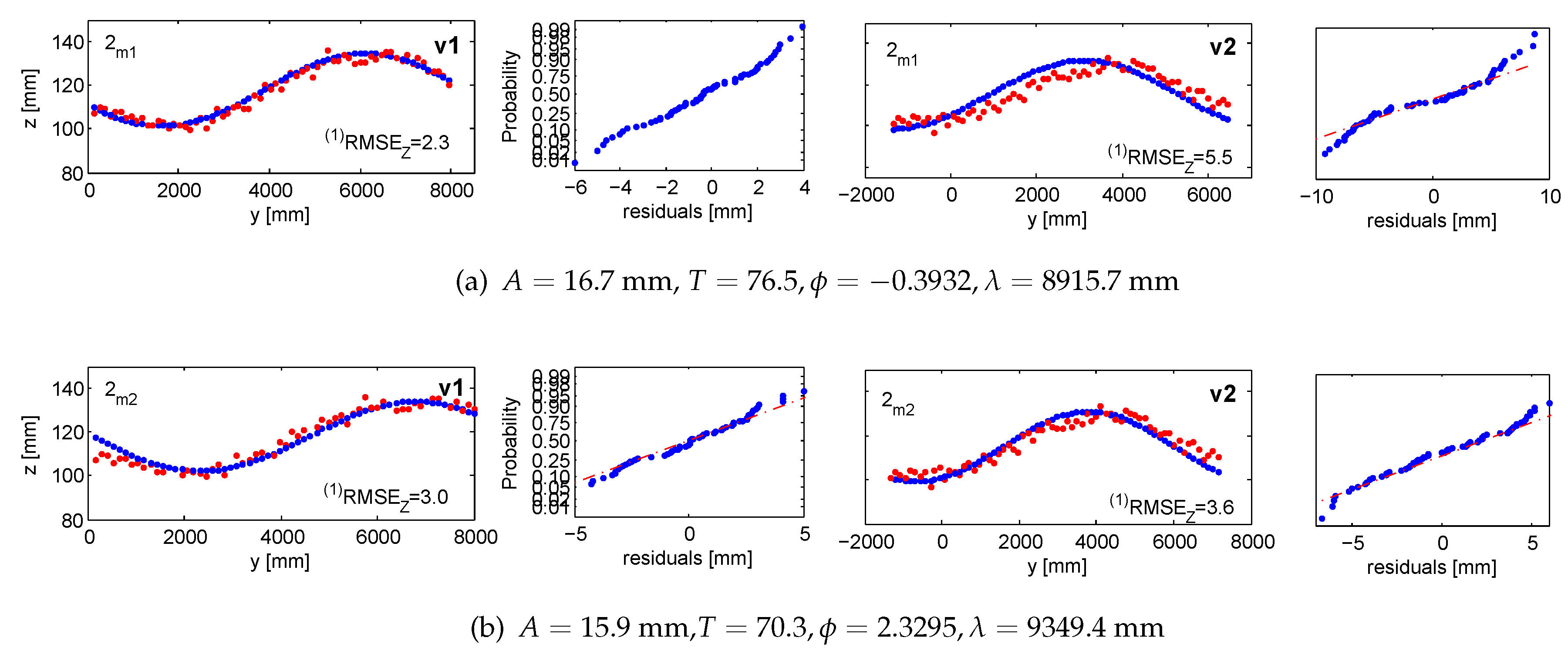
5. Experiments
5.1. Evaluation strategy
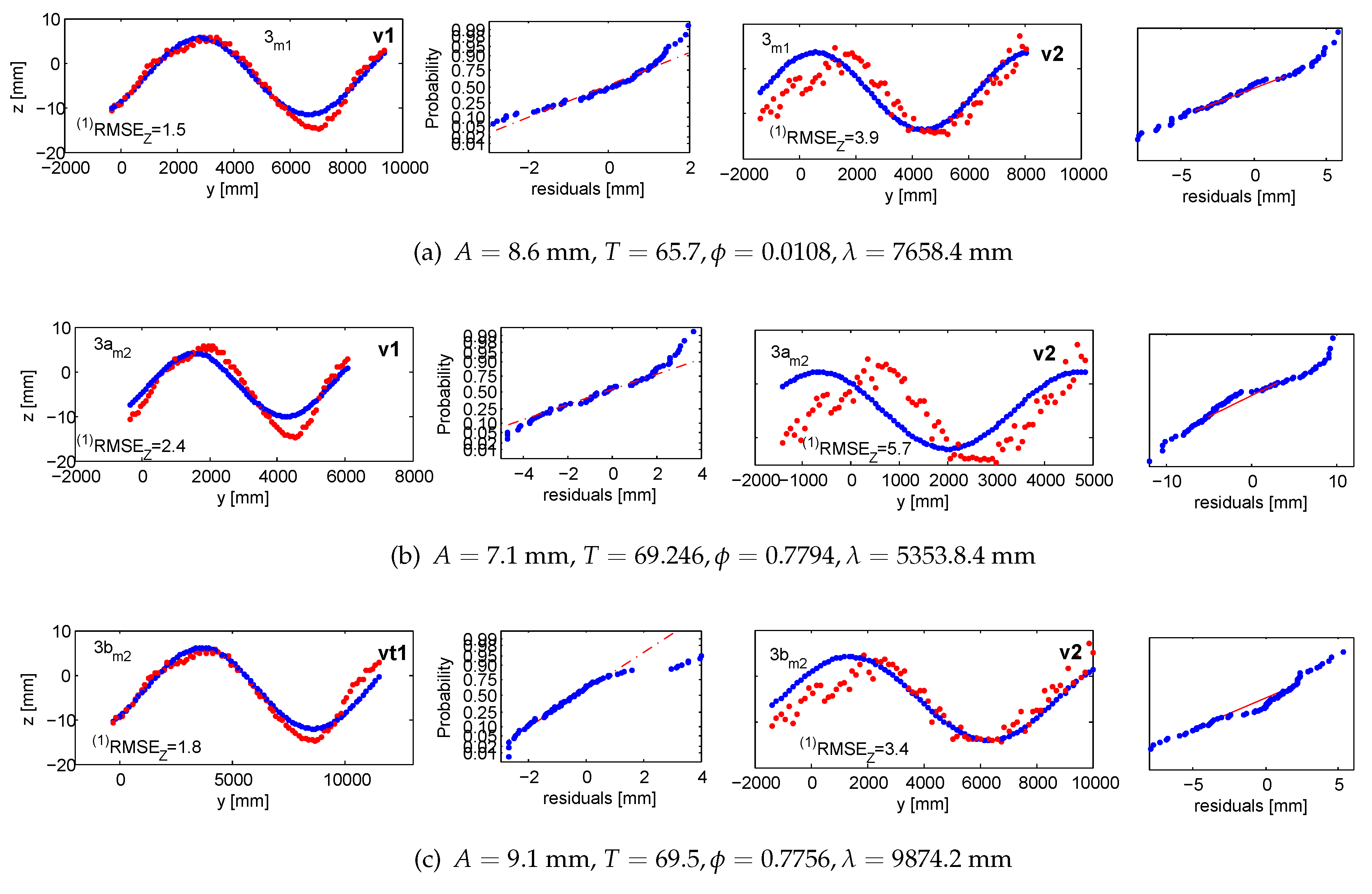
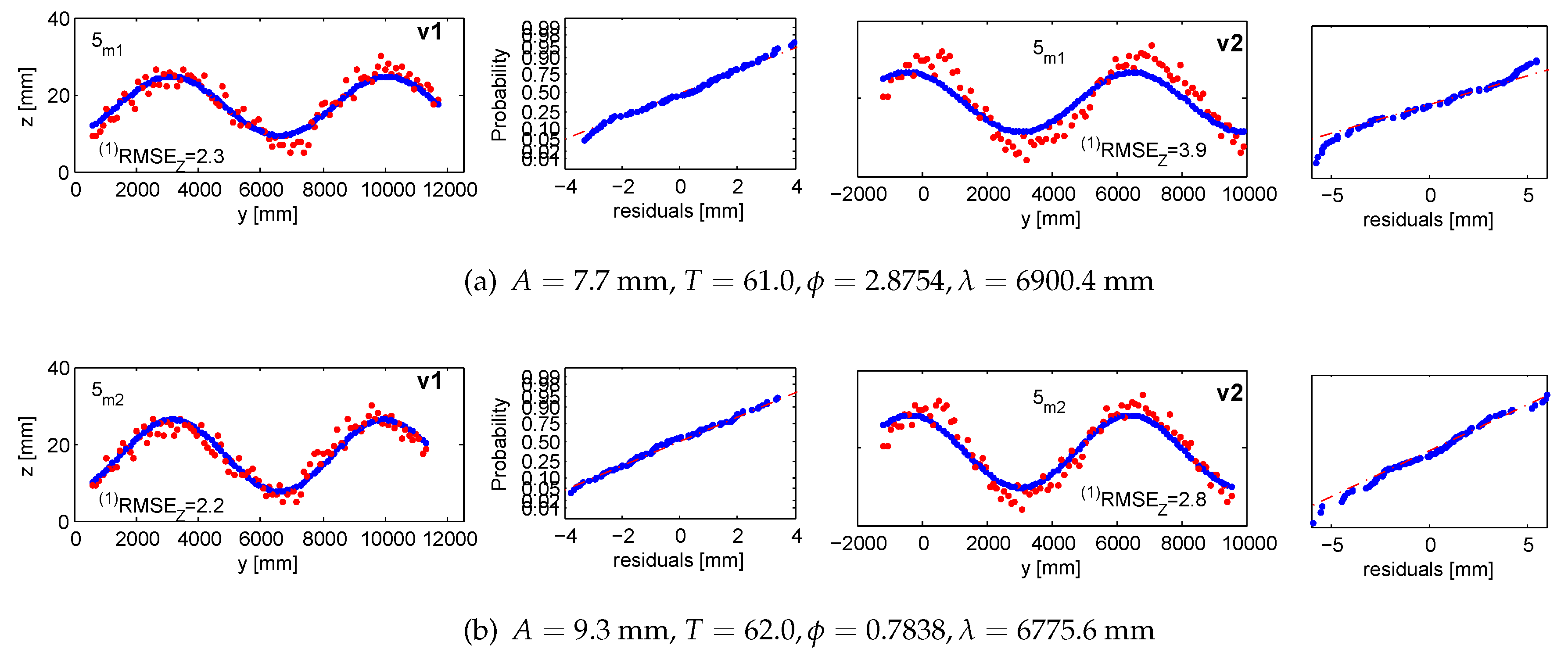
5.1.1. Accuracy 1: Validating Targets (, )
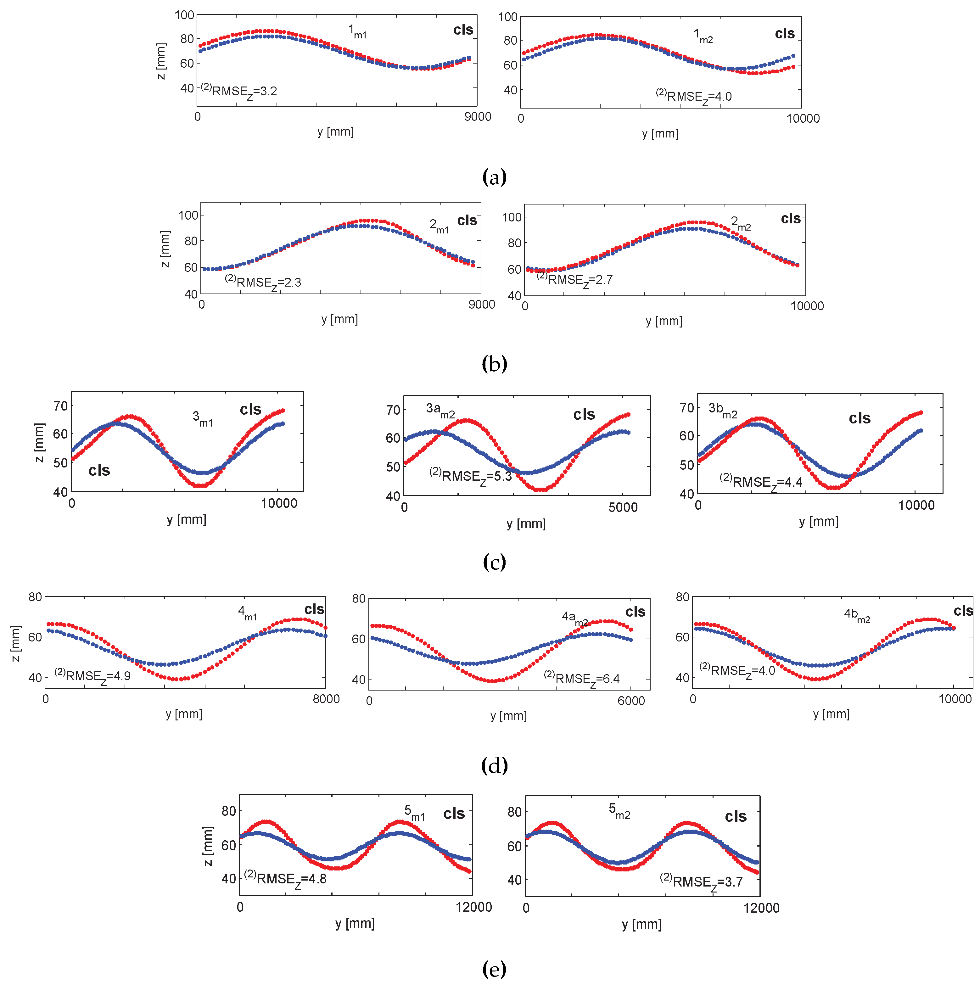
5.1.2. Accuracy 2: The Capacitive Level Sensor ()


5.2. Discussion
5.2.1. Accuracy
5.2.2. Precision
5.2.3. Wave Parameters
6. Conclusions
Acknowledgments
Author Contributions
Conflicts of Interest
Appendix A
References
- Kohlschütter, E. Stereophotogrammetrische Arbeiten, Wellen und Küstenaufnahmen. In Forschungsreise S.M.S Planet, 3; Verlag von Karl Siegismund: Berlin, Germany, 1906. (in German) [Google Scholar]
- Laas, W. Messung der Meereswellen und ihre Bedeutung für den Schiffbau. In Jahrbuch der Schiffbautechnischen Gesellschaft; Springer: Berlin, Germany, 1906; pp. 391–407. (in German) [Google Scholar]
- Waas, S. Entwicklung eines Verfahrens zur Messung kombinierter Höhen- und Neigungsverteilungen von Wasseroberflächenwellen mit Stereoaufnahmen. M.Sc. Thesis, Ruperto-Carola University of Heidelberg, Heidelberg, Germany, 1988. [Google Scholar]
- Kiefhaber, D. Optical Measurement of Short Wind Waves–From the Laboratory to the Field. Ph.D. Thesis, Ruperto-Carola University of Heidelberg, Heidelberg, Germany, 2014. [Google Scholar]
- Nocerino, E.; Ackermann, S.; Del Pizzo, S.; Menna, F.; Troisi, S. Low-cost human motion capture system for postural analysis onboard ships. In Proceedings of Videometrics, Range Imaging, and Applications XII, Munich, Germany, 14–15 May 2011; pp. 80850L–80856L.
- Stojic, M.; Chandler, J.; Ashmore, P.; Luce, J. The assessment of sediment transport rates by automated digital photogrammetry. Photogr. Eng. & Rem. Sens. 1998, 64, 387–395. [Google Scholar]
- Godding, R.; Hentschel, B.; Kauppert, K. Videometrie im wasserbaulichen Versuchswesen. Wasserwirtschaft, Wassertechnik 2003, 4, 36–40. (in German). [Google Scholar]
- Chandler, J.; Wackrow, R.; Sun, X.; Shiono, K.; Rameshwaran, P. Measuring a dynamic and flooding river surface by close range digital photogrammetry. In Proceedings of ISPRS Int. Arch. Photogram. Rem. Sens. Spat. Inform. Sci., Beijing, China, 3–11 July 2008; pp. 211–216.
- Mulsow, C.; Maas, H.G.; Westfeld, P.; Schulze, M. Triangulation methods for height profile measurements on instationary water surfaces. JAG 2008, 2, 21–29. [Google Scholar] [CrossRef]
- Adams, L.; Pos, J. Wave height measurements in model harbours using close range photogrammetry. In Proceedings of 15th Congress of the Int. Soc. for Photogram. Rem. Sens., Rio de Janeiro, Brazil, 17–29 June 1984.
- Redondo, J.; Rodriguez, A.; Bahia, E.; Falques, A.; Gracia, V.; Sánchez-Arcilla, A.; Stive, M. Image analysis of surf zone hydrodynamics. In Proceedings of International Conference on the Role of the Large Scale Experiments in Coastal Research, Barcelona, Spain, 21–25 February 1994.
- Aarninkhof, S.G.; Turner, I.L.; Dronkers, T.D.; Caljouw, M.; Nipius, L. A video-based technique for mapping intertidal beach bathymetry. Coast. Eng. 2003, 49, 275–289. [Google Scholar] [CrossRef]
- Santel, F. Automatische Bestimmung von Wasseroberflächen in der Brandungszone aus Bildsequenzen mittels digitaler Bildzuordnung. Ph.D Thesis, Fachrichtung Geodäsie und Geoinformatik University Hannover, Hannover, Germany, 2006. [Google Scholar]
- Jähne, B.; Klinke, J.; Waas, S. Imaging of short ocean wind waves: A critical theoretical review. J. Opt. Soc. Am. 1994, 11, 2197–2209. [Google Scholar] [CrossRef]
- Kiefhaber, D. Development of a Reflective Stereo Slope Gauge for the measurement of ocean surface wave slope statistics. M.Sc. Thesis, Ruperto-Carola University of Heidelberg, Heidelberg, Germany, 2010. [Google Scholar]
- Wahr, J.; Smeed, D.A.; Leuliette, E.; Swenson, S. Seasonal variability of the Red Sea, from satellite gravity, radar altimetry, and in situ observations. J. Geophys. Res. Oceans 2014, 119, 5091–5104. [Google Scholar] [CrossRef]
- Schiavulli, D.; Lenti, F.; Nunziata, F.; Pugliano, G.; Migliaccio, M. Landweber method in Hilbert and Banach spaces to reconstruct the NRCS field from GNSS-R measurements. Int. J. Remote Sens. 2014, 35, 3782–3796. [Google Scholar] [CrossRef]
- Rupnik, E.; Jansa, J. Off-the-shelf videogrammetry—A success story. In Proceedings of ISPRS Int. Arch. Photogram. Rem. Sens. Spat. Inform. Sci., Munich, Germany, 14–15 May 2014; Volume 43, pp. 99–105.
- Nayar, S.K.; Ikeuchi, K.; Kanade, T. Surface reflection: Physical and geometrical perspectives. IEEE Trans. Pat. Anal. Mach. Intel. 1991, 13, 611–634. [Google Scholar] [CrossRef]
- Park, J.; Kak, A.C. 3D modeling of optically challenging objects. IEEE Comp. Graph. 2008, 14, 246–262. [Google Scholar] [CrossRef] [PubMed]
- Maresca, J.W.; Seibel, E. Terrestrial photogrammetric measurements of breaking waves and longshore currents in the nearshore zone. Coast. Eng. 1976. [Google Scholar] [CrossRef]
- Piepmeier, J.A.; Waters, J. Analysis of stereo vision-based measurements of laboratory water waves. In Proceedings of Geoscience and Remote Sensing Symposium, Anchorage, Alaska, USA, 20–24 September 2004; Volume 5, pp. 3588–3591.
- Cobelli, P.J.; Maurel, A.; Pagneux, V.; Petitjeans, P. Global measurement of water waves by Fourier transform profilometry. Exp. Fluids 2009, 46, 1037–1047. [Google Scholar] [CrossRef]
- Bhat, D.N.; Nayar, S.K. Stereo in the Presence of Specular Reflection. In Proceedings of the 5th International Conference on Computer Vision (ICCV), Boston, Massachusetts, USA, 20–23 June 1995; pp. 1086–1092.
- Wells, J.M.; Danehy, P.M. Polarization and Color Filtering Applied to Enhance Photogrammetric Measurements of Reflective Surface. In Proceedings of Structures, Structural Dynamics and Materials Conference, Austin, TX, USA, 18–21 April 2005.
- Black, J.T.; Blandino, J.R.; Jones, T.W.; Danehy, P.M.; Dorrington, A.A. Dot-Projection Photogrammetry and Videogrammetry of Gossamer Space Structures. Technical Report NASA/TM-2003-212146; NASA Langley Research Center: Hampton, VA, USA, 2003. [Google Scholar]
- Lippmann, T.; Holman, R. Wave group modulations in cross-shore breaking patterns. Coastal Eng. 1992. [Google Scholar] [CrossRef]
- Cox, C.; Munk, W. Measurement of the roughness of the sea surface from photographs of the sun’s glitter. J. Opt. Soc. Am. 1954, 44, 838–850. [Google Scholar] [CrossRef]
- Schooley, A.H. A simple optical method for measuring the statistical distribution of water surface slopes. J. Opt. Soc. Am. 1954, 44, 37–40. [Google Scholar] [CrossRef]
- Stilwell, D. Directional energy spectra of the sea from photographs. J. Geophys. Res. 1969, 74, 1974–1986. [Google Scholar] [CrossRef]
- Ikeuchi, K. Determining Surface Orientation of Specular Surfaces by Using the Photometric Stereo Method. IEEE Trans. Pat. Anal. Mach. Intel. 1981, 3, 661–669. [Google Scholar] [CrossRef]
- Healey, G.; Binford, T.O. Local shape from specularity. Comput. Vis. Graph. Image Process. 1988, 42, 62–86. [Google Scholar] [CrossRef]
- Sanderson, A.C.; Weiss, L.E.; Nayar, S.K. Structured highlight inspection of specular surfaces. IEEE Trans. Pat. Anal. Mach. Intel. 1988, 10, 44–55. [Google Scholar] [CrossRef]
- Halstead, M.A.; Barsky, B.A.; Klein, S.A.; Mandell, R.B. Reconstructing curved surfaces from specular reflection patterns using spline surface fitting of normals. In Proceedings of the 23rd Annual Conference on Computer Graphics and Interactive Techniques, New Orleans, LA, USA, 4–9 August 1996; pp. 335–342.
- Savarese, S.; Perona, P. Local analysis for the 3rd reconstruction of specular surfaces. Comp. Vis. Pat. Recog. 2001, 2, 738–745. [Google Scholar]
- Bonfort, T.; Sturm, P. Voxel carving for specular surfaces. In Proceedings of the 9th International Conference on Computer Vision (ICCV), Nice, France, 13–16 October 2003; pp. 591–596.
- Roth, S.; Black, M.J. Specular flow and the recovery of surface structure. IEEE Comp. Soc. Conf. Comp. Vis. Pat. Recog. 2006, 2, 1869–1876. [Google Scholar]
- Adato, Y.; Vasilyev, Y.; Ben-Shahar, O.; Zickler, T. Toward a theory of shape from specular flow. In Proceedings of IEEE 11th International Conference on Computer Vision, Rio de Janeiro, Brazil, 14–21 October 2007; pp. 1–8.
- Sankaranarayanan, A.C.; Veeraraghavan, A.; Tuzel, O.; Agrawal, A. Specular surface reconstruction from sparse reflection correspondences. In Proceedings of IEEE 23rd Conference on Computer Vision and Pattern Recognition, San Francisco, LA, USA, 13–18 June 2010; pp. 1245–1252.
- Kutulakos, K.N.; Steger, E. A theory of refractive and specular 3d shape by light-path triangulation. Int. J. Comp. Vis. 2008, 76, 13–29. [Google Scholar] [CrossRef]
- Ma, W.C.; Hawkins, T.; Peers, P.; Chabert, C.F.; Weiss, M.; Debevec, P. Rapid acquisition of specular and diffuse normal maps from polarized spherical gradient illumination. In Proceedings of the 18th Eurographics conference on Rendering Techniques, Eurographics Association, Aire-la-Ville, Switzerland, 2007; pp. 183–194.
- Stolz, C.; Ferraton, M.; Meriaudeau, F. Shape from polarization: A method for solving zenithal angle ambiguity. Opt. Let. 2012, 37, 4218–4220. [Google Scholar] [CrossRef] [PubMed]
- Hertzmann, A.; Seitz, S.M. Example-based photometric stereo: Shape reconstruction with general, varying brdfs. IEEE Trans. Pat. Anal. Mach. Intel. 2005, 27, 1254–1264. [Google Scholar] [CrossRef] [PubMed]
- Lensch, H.P.A.; Kautz, J.; Goesele, M.; Heidrich, W.; Seidel, H.P. Image-based Reconstruction of Spatial Appearance and Geometric Detail. ACM Trans. Graph. 2003, 22, 234–257. [Google Scholar] [CrossRef]
- Wang, J.; Dana, K.J. Relief texture from specularities. IEEE Trans. Pat. Anal. Mach. Intel. 2006, 28, 446–457. [Google Scholar]
- Meriaudeau, F.; Sanchez Secades, L.; Eren, G.; Ercil, A.; Truchetet, F.; Aubreton, O.; Fofi, D. 3D Scanning of Non-Opaque Objects by means of Imaging Emitted Structured Infrared Patterns. IEEE Trans. Instrum. Meas. 2010, 59, 2898–2906. [Google Scholar] [CrossRef]
- Eren, G.; Aubreton, O.; Meriaudeau, F.; Sanchez Secades, L.A.; Fofi, D.; Truchetet, F.; Ercil, A. Scanning From Heating: 3D Shape Estimation of Transparent Objects from Local Surface Heating. Opt. Express 2009, 17, 11457–11468. [Google Scholar] [CrossRef] [PubMed]
- Hilsenstein, V. Design and implementation of a passive stereo-infrared imaging system for the surface reconstruction of Water Waves. Ph.D Thesis, Ruperto-Carola University of Heidelberg, Heildeberg, Germany, 2004. [Google Scholar]
- Rantoson, R.; Stolz, C.; Fofi, D.; Mériaudeau, F. 3D reconstruction of transparent objects exploiting surface fluorescence caused by UV irradiation. In Proceedings of 17th IEEE International Conference on Image Processing, Hong Kong, 26–29 September 2010; pp. 2965–2968.
- Ihrke, I.; Kutulakos, K.N.; Lensch, H.P.; Magnor, M.; Heidrich, W. State of the art in transparent and specular object reconstruction. EUROGRAPHICS STAR 2008. [Google Scholar]
- Morris, N.J. Shape Estimation under General Reflectance and Transparency. PhD Thesis, University of Toronto, Toronto, Ontario, Canada, 2011. [Google Scholar]
- Cox, C.S. Measurement of slopes of high-frequency wind waves. J. Mar. Res. 1958, 16, 199–225. [Google Scholar]
- Jähne, B.; Riemer, K. Two-dimensional wave number spectra of small-scale water surface waves. J. Geophys. Res.: Oceans (1978–2012) 1990, 95, 11531–11546. [Google Scholar] [CrossRef]
- Zhang, X.; Cox, C.S. Measuring the two-dimensional structure of a wavy water surface optically: A surface gradient detector. Exp. Fluids 1994, 17, 225–237. [Google Scholar] [CrossRef]
- Rocholz, R. Spatiotemporal Measurement of Shortwind-Driven Water Waves. Ph.D Thesis, Ruperto-Carola University of Heidelberg, Heidelberg, Germany, 2008. [Google Scholar]
- Sturtevant, B. Optical depth gauge for laboratory studies of water waves. Rev. Scient. Instr. 1966, 37. [Google Scholar] [CrossRef]
- Hughes, B.; Grant, H.; Chappell, R. A fast response surface-wave slope meter and measured wind-wave moments. Deep Sea Res. 1977, 24, 1211–1223. [Google Scholar] [CrossRef]
- Bock, E.J.; Hara, T. Optical measurements of capillary-gravity wave spectra using a scanning laser slope gauge. J. Atm. Ocean. Tech. 1995, 12, 395–403. [Google Scholar] [CrossRef]
- Murase, H. Surface Shape Recontruction of a Nonrigid Transparent Object Using Refraction and Motion. IEEE Trans. Pat. Anal. Mach. Intel. 1992, 14, 1045–1052. [Google Scholar] [CrossRef]
- Morris, N.J.; Kutulakos, K.N. Dynamic Refraction Stereo. IEEE Trans. Pat. Anal. Mach. Intel. 2011, 33, 1518–1531. [Google Scholar] [CrossRef] [PubMed]
- Shortis, M.R.; Clarke, T.A.; Robson, S. Practical testing of the precision and accuracy of target image centering algorithms. Videometrics IV, SPIE: Philadelphia, PA, USA,, October 1995; pp. 65–76. [Google Scholar]
- Otepka, J. Precision Target Mensuration in Vision Metrology. Ph.D Thesis, Technische Universtiät Wien, Wien, Austria, 2004. [Google Scholar]
- Wiora, G.; Babrou, P.; Männer, R. Real time high speed measurement of photogrammetric targets. In Pattern Recognition; Springer: Berlin Heidelberg, Germany, 2004; pp. 562–569. [Google Scholar]
- Kraus, K. Photogrammetry. In Advanced Methods and Applications; Dümmler Verlag: Bonn, Germany, 1997; Volume 2. [Google Scholar]
- Rusu, R.B. Semantic 3D Object Maps for Everyday Manipulation in Human Living Environments. Ph.D Thesis, Computer Science department, Technische Universität Muenchen, Munich, Germany, 2009. [Google Scholar]
- Point Cloud Library (PCL). Available online: http://pointclouds.org/ (accessed on November 2014).
- Blake, A.; Brelstaff, G. Geometry From Specularities. In Proceedings of International Conference on Computer Vision (ICCV), Tampa, Florida, USA, December 1988; pp. 394–403.
- MicMac, Apero, Pastis and Other Beverages in a Nutshell! Available online: http://logiciels.ign.fr/?Telechargement (accessed on 20 March 2015).
- Deseilligny-Pierrot, M.; Clery, I. Apero, an open source bundle adjustment software for automatic calibration and orientation of set of images. ISPRS Int. Arch. Photogram. Rem. Sens. Spat. Inform. Sci. 2011, 38, 269–276. [Google Scholar]
- Maas, H.G. Image sequence based automatic multi-camera system calibration techniques. J. Photogram. Rem. Sens. 1999, 54, 352–359. [Google Scholar] [CrossRef]
© 2015 by the authors; licensee MDPI, Basel, Switzerland. This article is an open access article distributed under the terms and conditions of the Creative Commons by Attribution (CC-BY) license (http://creativecommons.org/licenses/by/4.0/).
Share and Cite
Rupnik, E.; Jansa, J.; Pfeifer, N. Sinusoidal Wave Estimation Using Photogrammetry and Short Video Sequences. Sensors 2015, 15, 30784-30809. https://doi.org/10.3390/s151229828
Rupnik E, Jansa J, Pfeifer N. Sinusoidal Wave Estimation Using Photogrammetry and Short Video Sequences. Sensors. 2015; 15(12):30784-30809. https://doi.org/10.3390/s151229828
Chicago/Turabian StyleRupnik, Ewelina, Josef Jansa, and Norbert Pfeifer. 2015. "Sinusoidal Wave Estimation Using Photogrammetry and Short Video Sequences" Sensors 15, no. 12: 30784-30809. https://doi.org/10.3390/s151229828
APA StyleRupnik, E., Jansa, J., & Pfeifer, N. (2015). Sinusoidal Wave Estimation Using Photogrammetry and Short Video Sequences. Sensors, 15(12), 30784-30809. https://doi.org/10.3390/s151229828