
Smart Building: Decision Making Architecture for Thermal Energy Management

 ,
,  and
and
Abstract
:
1. Introduction
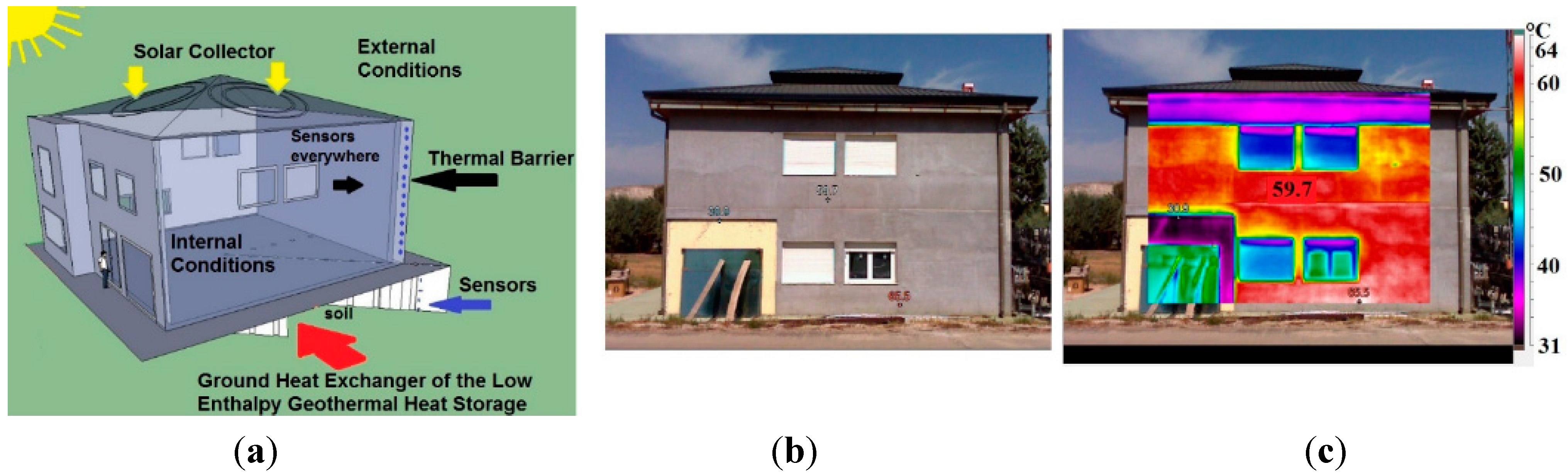
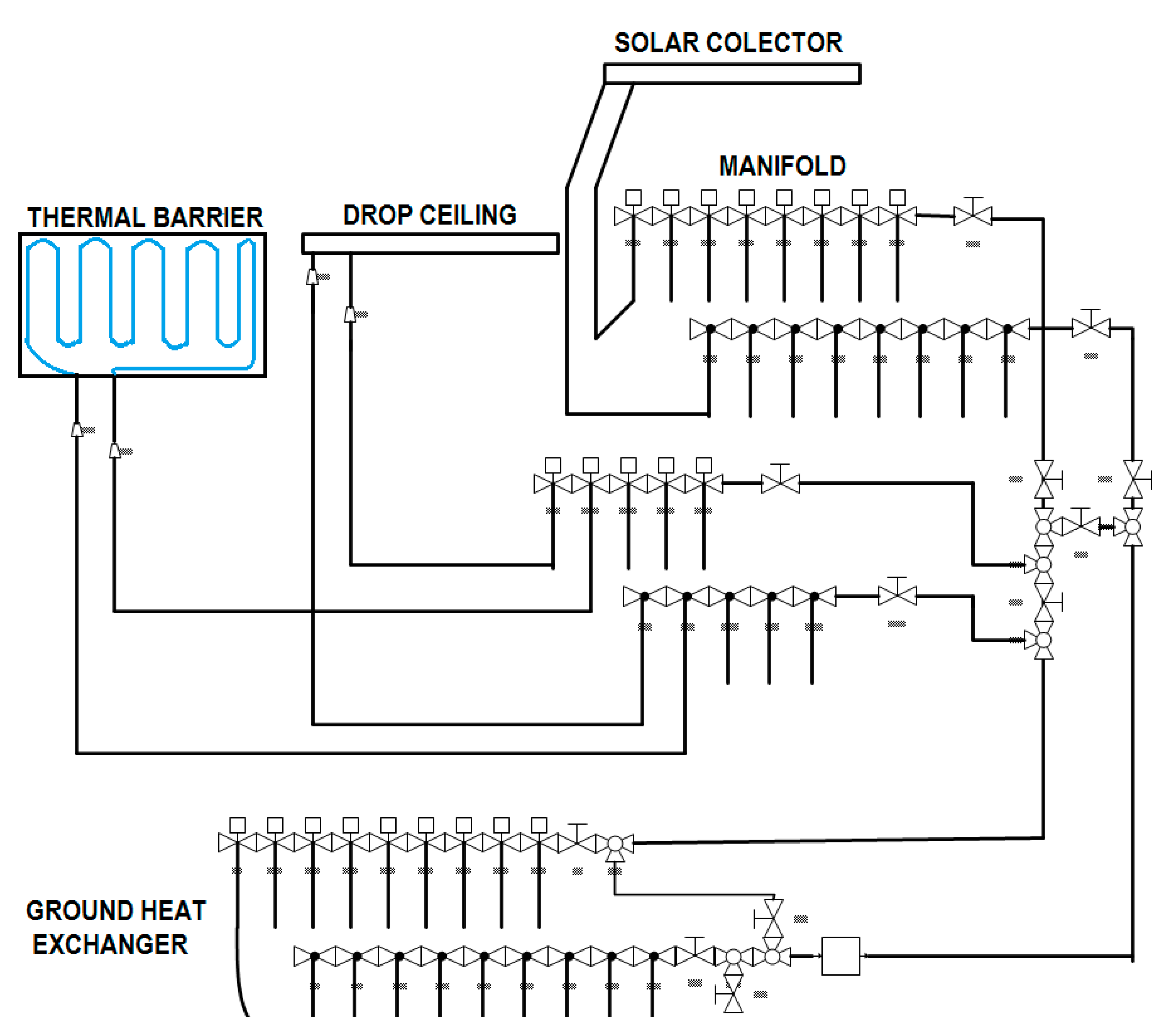
2. Thermal Energy Acquisition, Storage and Transfer Systems
- The solar collector (located in the roof)
- The low enthalpy geothermal heat store (ground heat exchanger)
- The dynamic thermal barrier (walls)

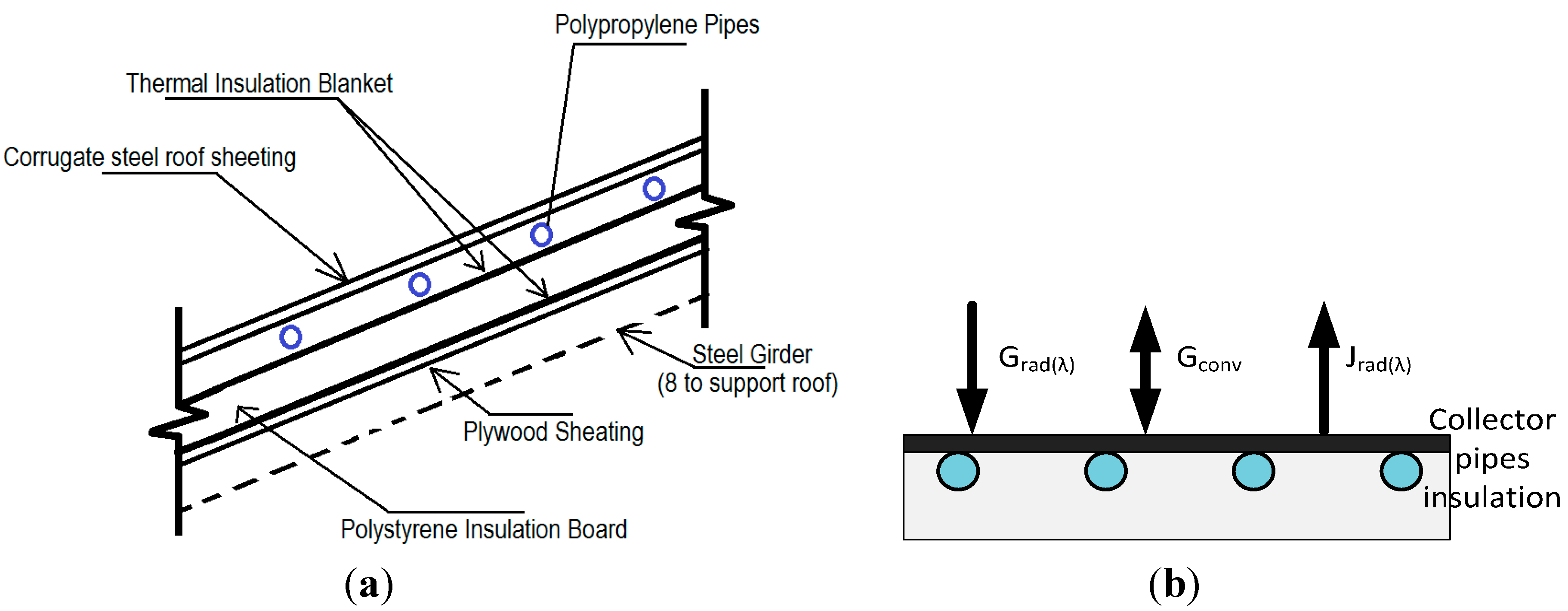
2.1. Thermal Solar Energy Collector

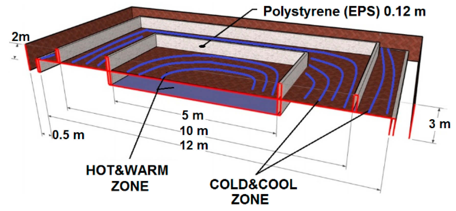
2.2. Ground Heat Exchanger: Low Enthalpy Horizontal Ground Thermal Energy Source


| Temperature | Range | Characteristics |
|---|---|---|
| HOT | 19–21 °C | 2 PP pipes, 0.22 m, L 200 m, located 3 m underground, buried below the building |
| WARM | 17–19 °C | 2 PP pipes, 0.22 m, L 200 m, located 2 m underground, buried below the building |
| COOL | 15–17 °C | 3 PP pipes, 0.22 m, L 200 m, located 2 m underground, buried below the building |
| COLD | 12–15 °C | 2 PP pipes, 0.22 m, L 200 m, located 2m underground, buried outside the building |
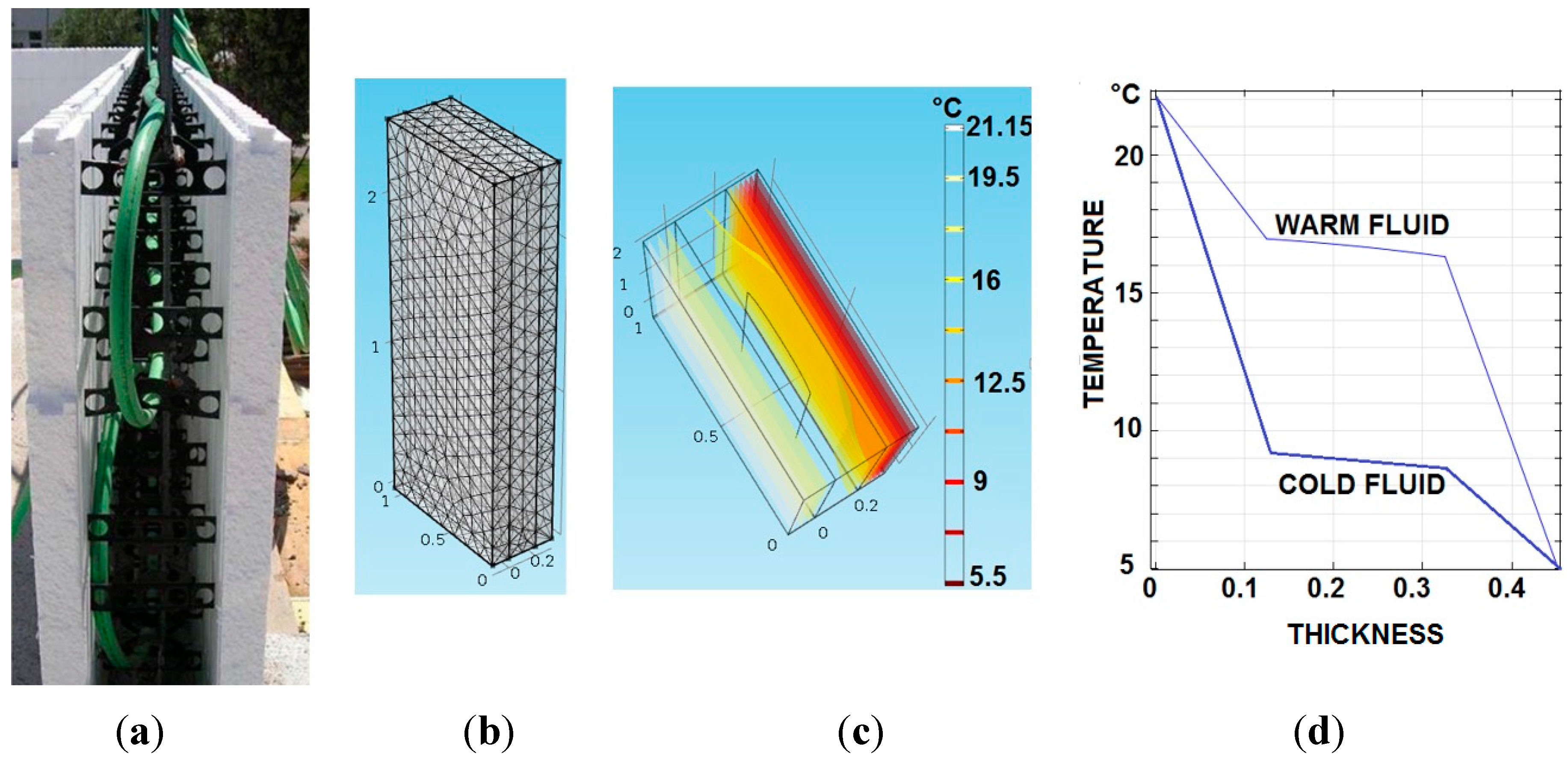
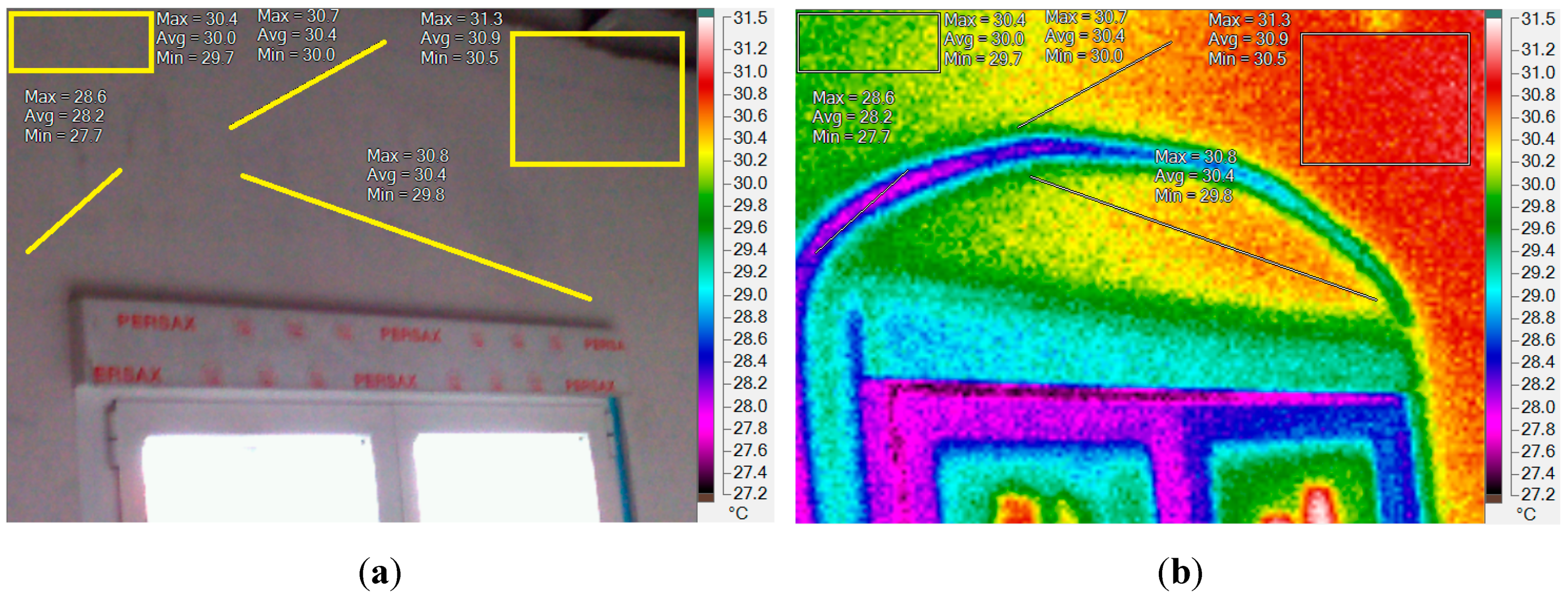
2.3. Dynamic Envelope: Thermal Barrier
| Lightweight Concrete | Value | Units |
|---|---|---|
| Thickness | 0.15 | m |
| Density | 1200 | kg/m3 |
| Specific Heat | 800 | J/kg·K |
| Thermal Conductivity | 0.57 | W/m·K |
| POLYSTYRENE | ||
| Thickness | 0.05 | m |
| Density | 35 | kg/m3 |
| Specific Heat | 1450 | J/kg·K |
| Thermal Conductivity | 0.036 | W/m·K |
| nZEB | ||
| House Height | 5 | m |
| House Width | 10 | m |
| House Length | 10 | m |
| Windows | 15 | |
| Window Height | 1 | m |
| Window Width | 1 | M |
| Window Density | 2500 | kg/m3 |
| Window Specific Heat | 840 | J/kg·K |
| Window Thermal Cond. | 0.78 | W/m·K |
| Initial Temperature | 7.5 | °C |

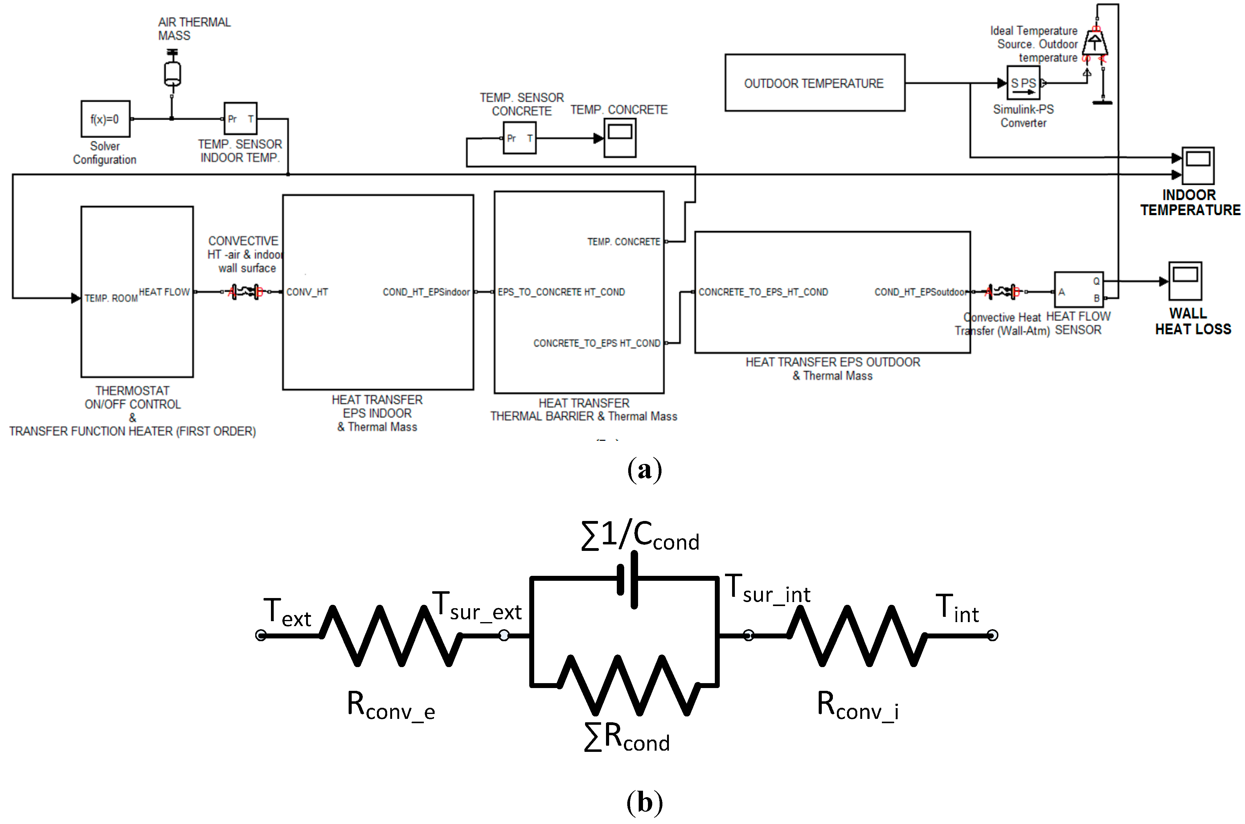

2.4. Hydraulic Circuit

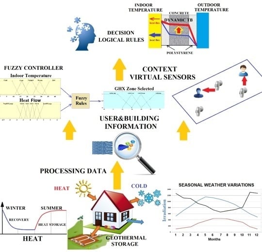
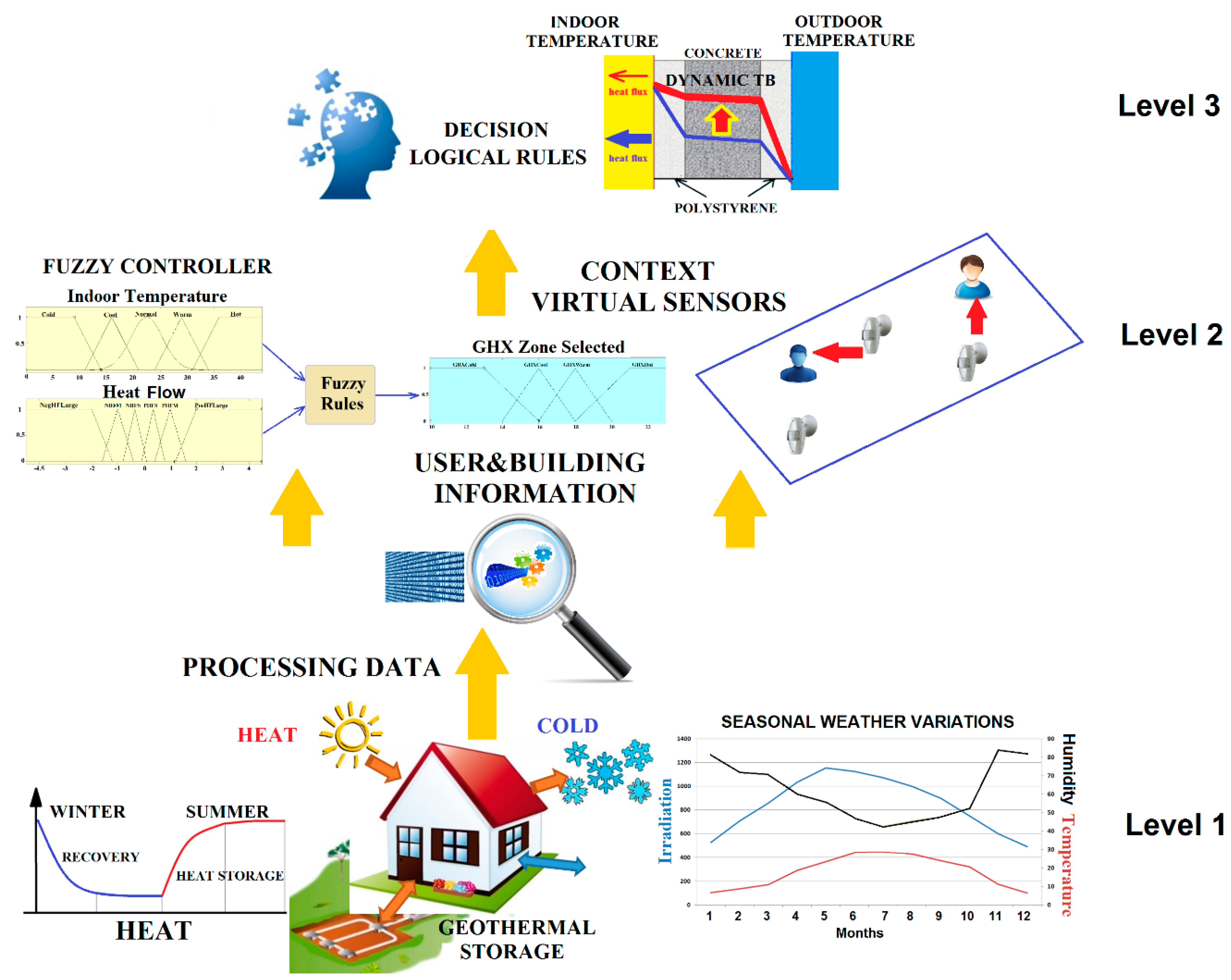
3. Smart Building: A Perceptual and Decision-Making Architecture for Thermal Energy Management

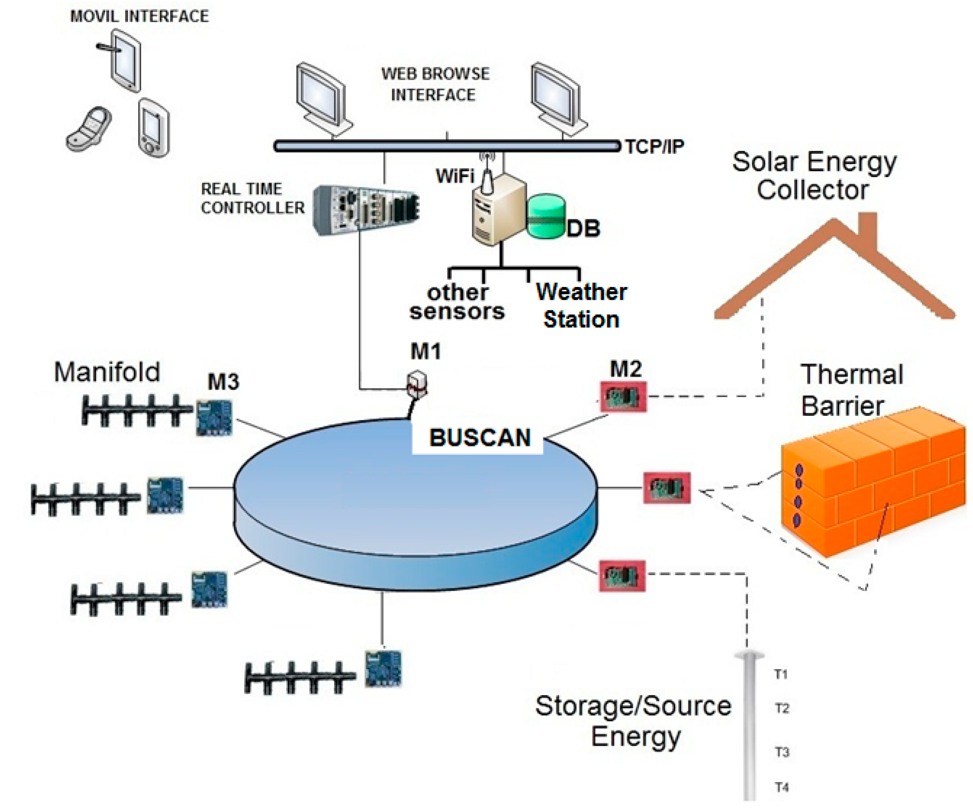
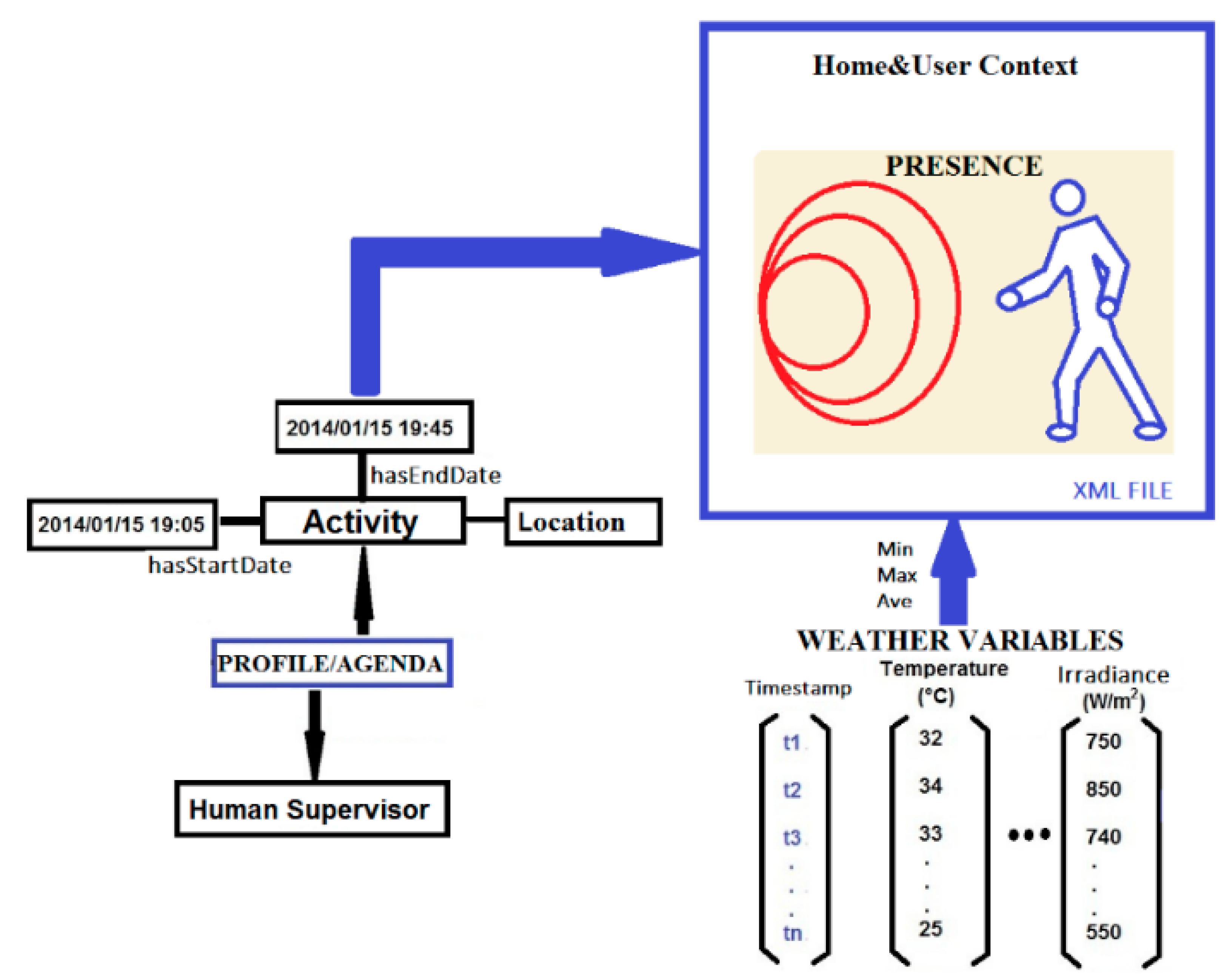
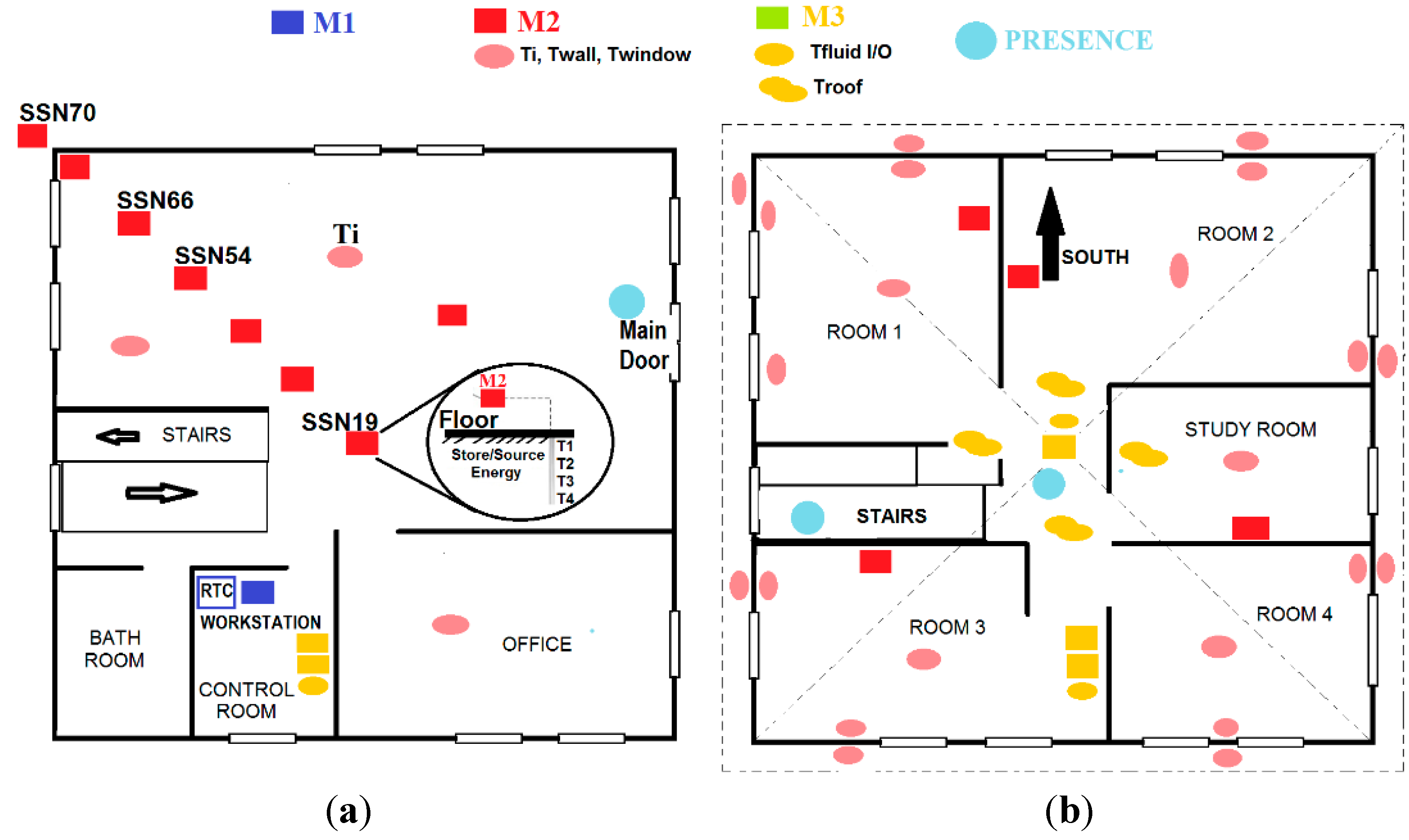
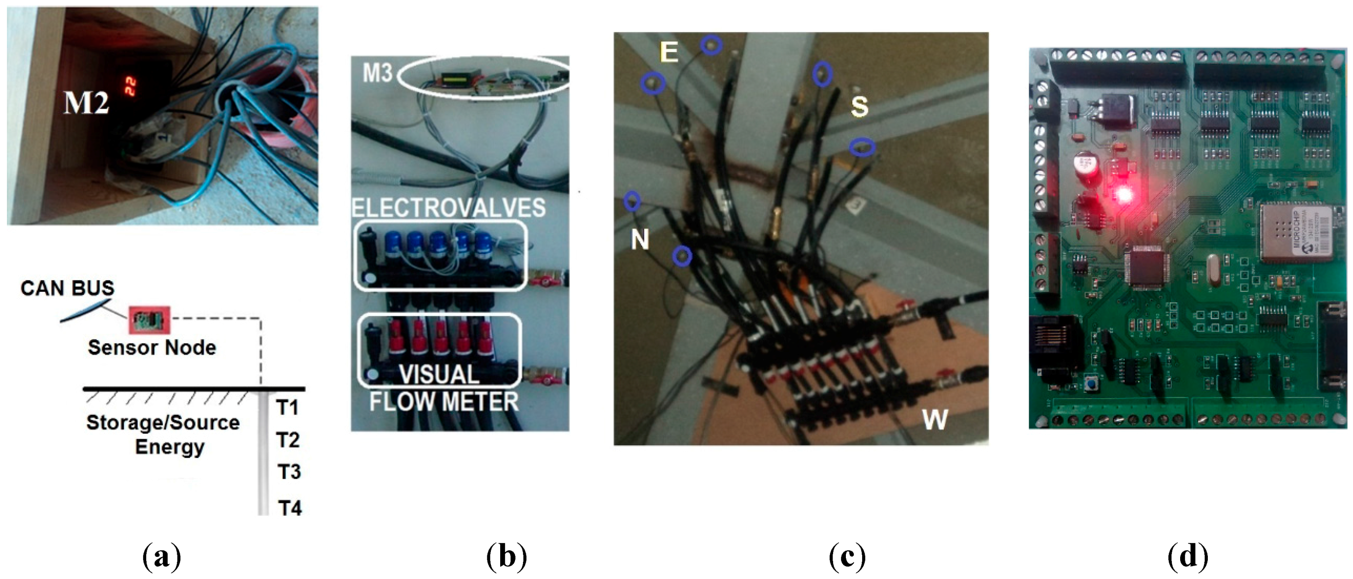
3.1. Level 1: Sensor and Communication Layer
- M1: IoT gateway module.
- M2: IoT nodes dedicated to monitoring temperatures at different locations: indoor temperature (Ti), subsurface probes (Ts), walls (TW), and windows (Tw).
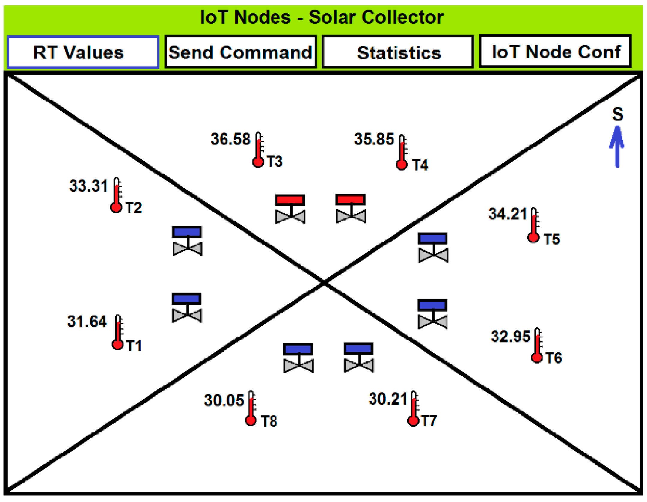
- M3: IoT actuator nodes, acting on the valves and monitoring the volumetric flow rate. They measure both fluid and roof's faces temperatures and provide web service functionalities through a TCP/IP stack and a light web server. The embedded web pages are stored in low resolution, to support commands and exchange information with end users.
- Real Time Controller (RTC): main control system with VxWorks operating system, and web server.
- Workstation and Data Base (DB): workstation is mainly used to exchange data and information with the Real Time Controller (RTC) but also to get data from other sensors. A DB is used to store data for further processing.
- Other sensors, mainly presence sensors.
- Weather station: weather variables such as solar irradiation and outdoor humidity.
- Mobile and Web Interface: the RTC and M3 IoT actuator nodes have a Web Server to show information by opening a web browser on mobile applications.


3.2. Level 2: User and Building Information Layer
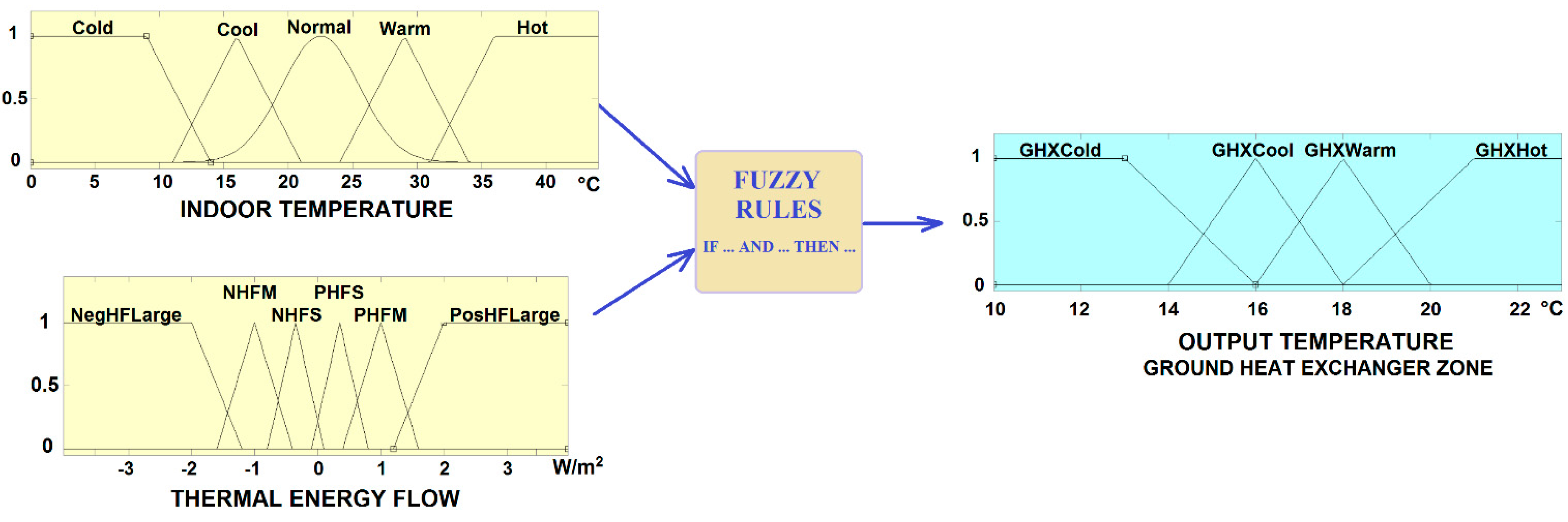
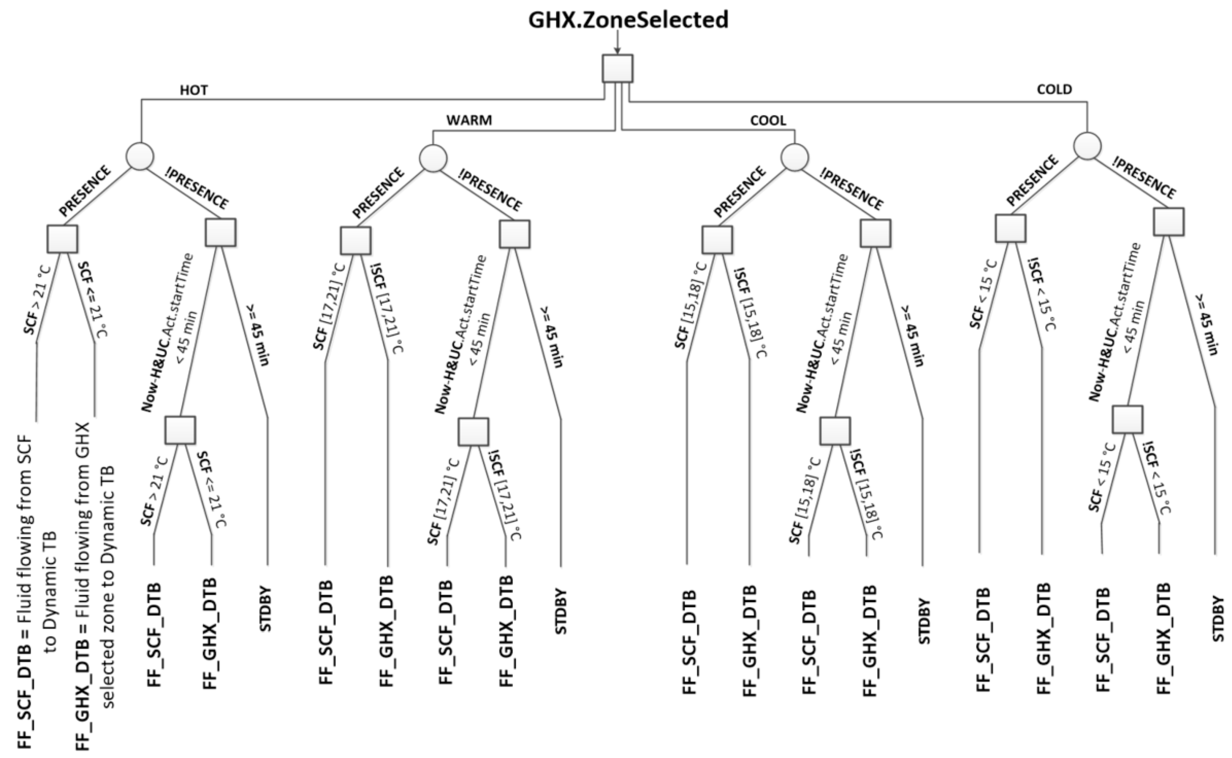
3.2.1. The Fuzzy Controller

| Temperature/Thermal Flow | NegHF Large | NHFM | NHFS | PHFS | PHFM | PosHF Large |
|---|---|---|---|---|---|---|
| COLD | GHXHot | GHXWarm | GHXCool | GHXCold | GHXCool | GHXHot |
| COOL | GHXHot | GHXHot | GHXHot | GHXWarm | GHXWarm | GHXCool |
| NORMAL | GHXCool | GHXWarm | GHXHot | GHXHot | GHXHot | GHXWarm |
| WARM | GHXCool | GHXWarm | GHXHot | GHXHot | GHXHot | GHXHot |
| HOT | GHXCold | GHXCold | GHXCool | GHXWarm | GHXCool | GHXCold |
3.2.2. Thermal Barrier and Home and User Context Virtual Sensors
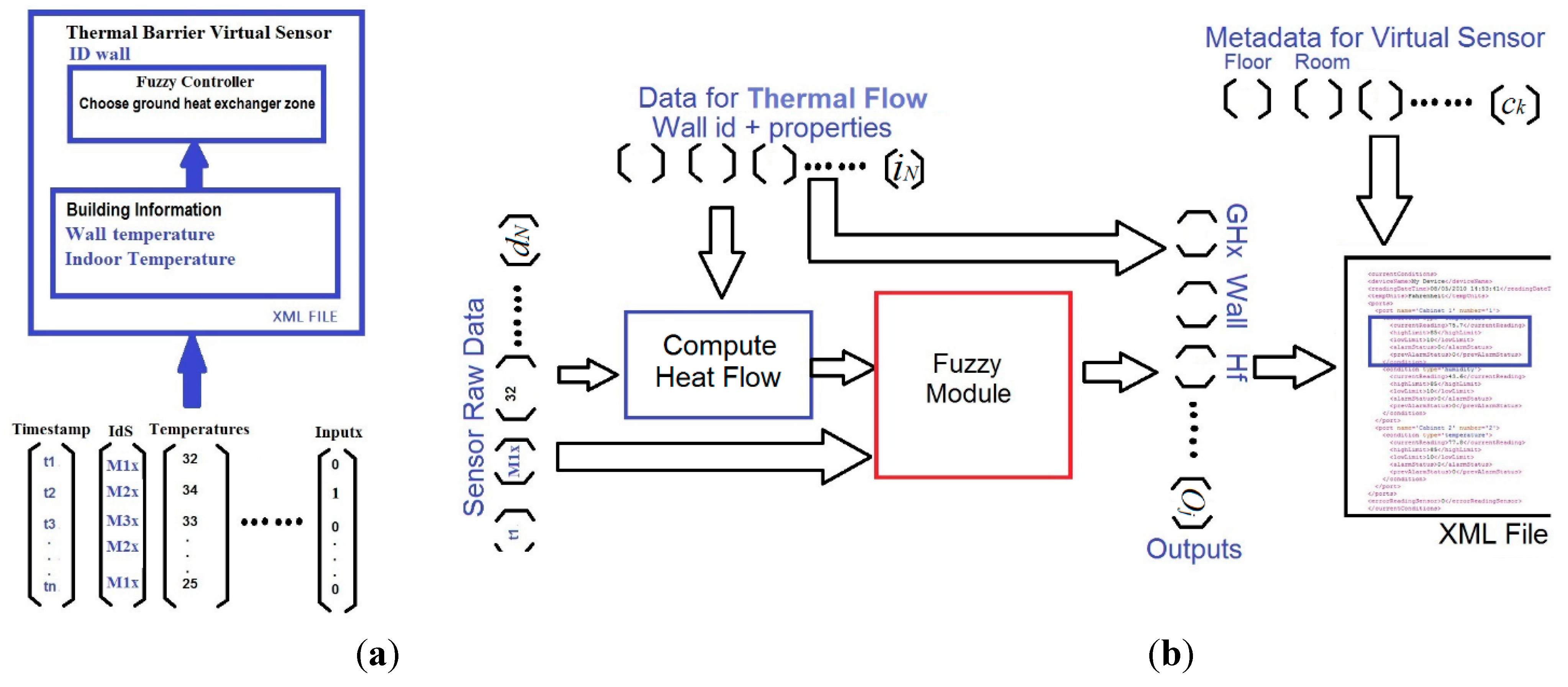

3.3. Level 3: Decision Layer
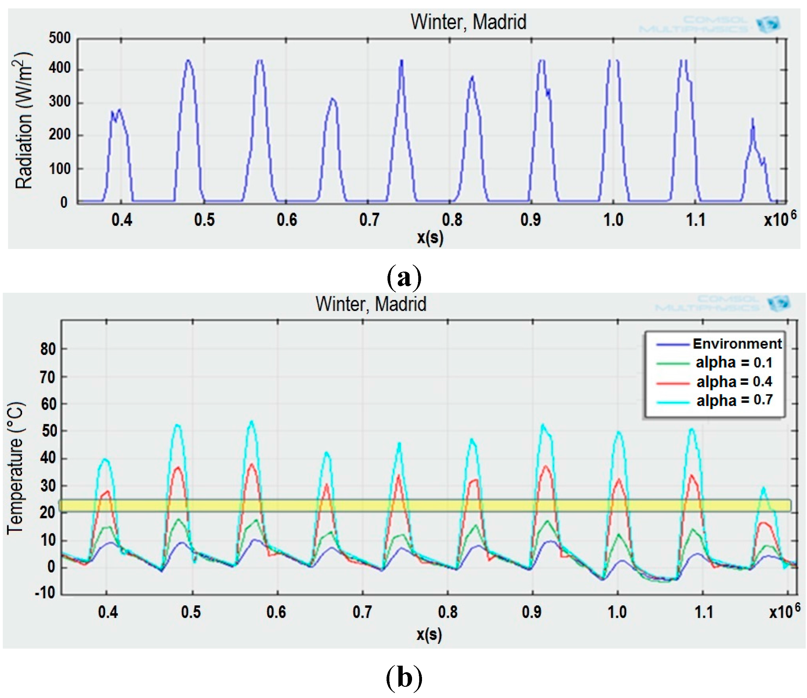
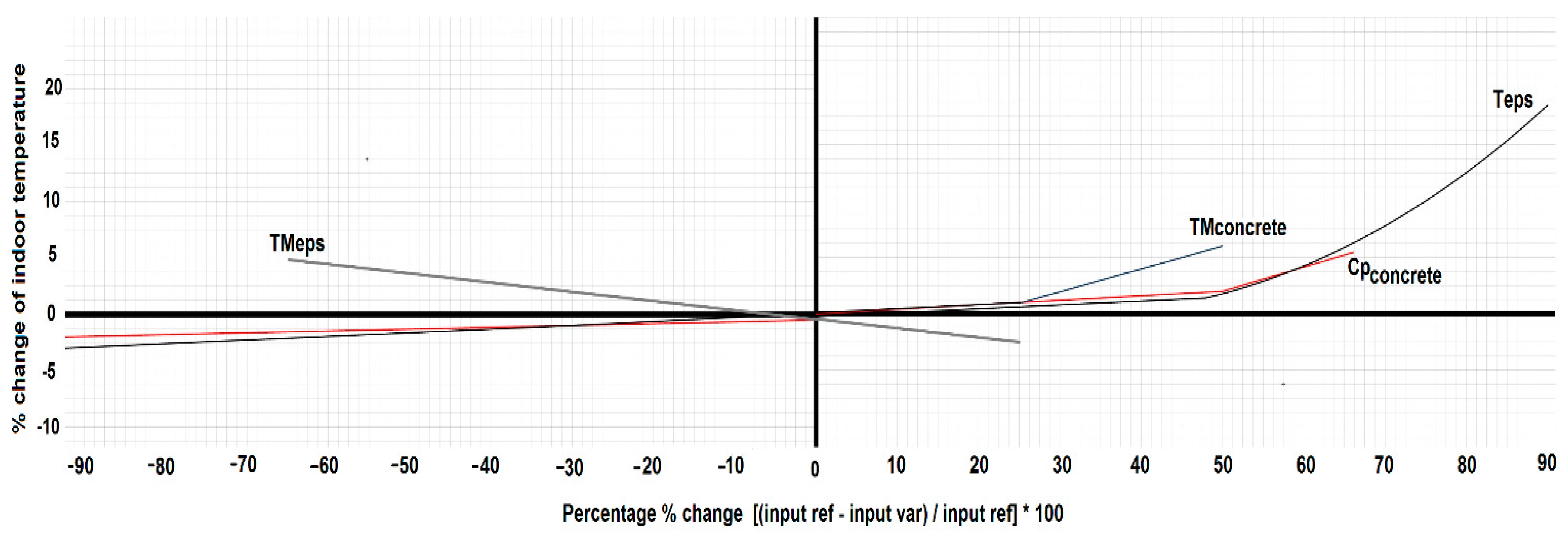
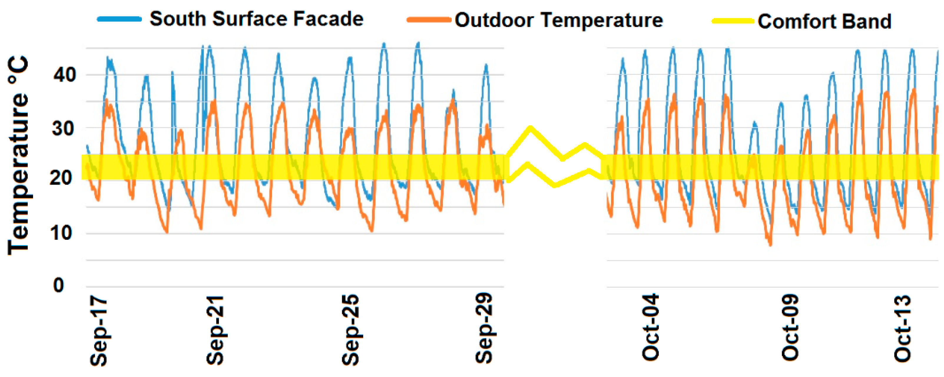
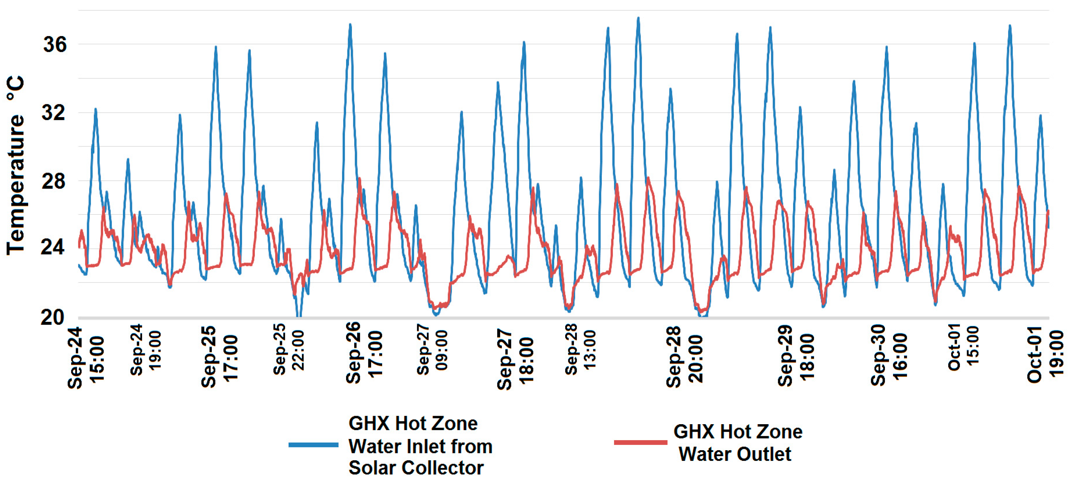
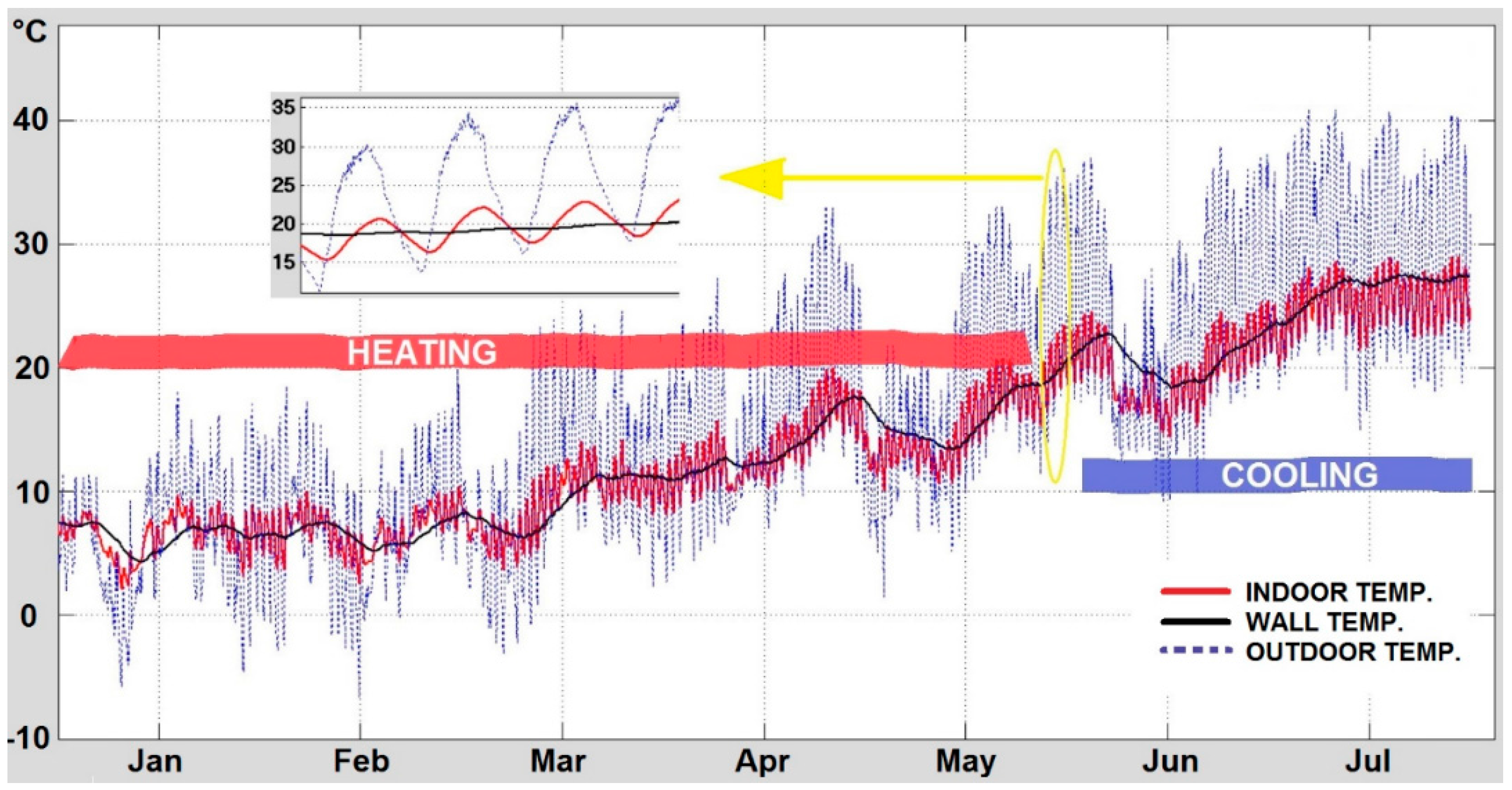
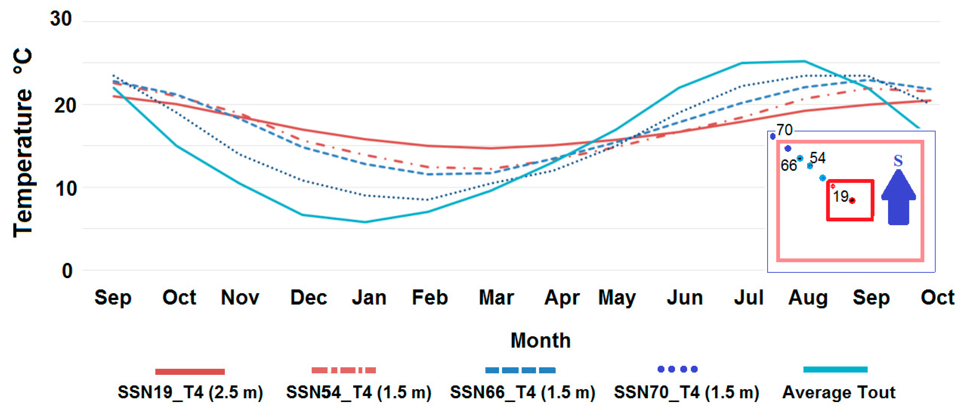
4. Experimental Results and Discussion


5. Conclusions
Acknowledgments
Author Contributions
Conflicts of Interest
References
- Bio Intelligence Service; Ronan, L.; IEEP. Energy Performance Certificates in Buildings and Their Impact on Transaction Prices and Rents in Selected EU Countries; Technical Report for European Commission (DG Energy): Brussels, Belgium, April 2013. [Google Scholar]
- Victor, D.G.; Zhou, D.; Ahmed, E.H.M.; Dadhich, P.K.; Olivier, J.; Rogner, H-H.; Sheikho, K.; Yamaguchi, M. Introductory chapter. In Climate Change 2014: Mitigation of Climate Change. Contribution of Working Group III to the Fifth Assessment Report of the IPCC; Cambridge University Press: Cambridge, UK, 2014. [Google Scholar]
- Bogdan, A.; Ecofys Germany GmbH; SBi. Principles for Nearly Zero Energy Buildings: Paving the Way for Effective Implementation of Policy Requirements; Buildings Performance Institute Europe: Brussels, Belgium, November 2011. [Google Scholar]
- Beerepoot, M. Technology Roadmap Solar Heating and Cooling; OECD/IEA: Paris, France, 2012. [Google Scholar]
- Jin, X.; Zhang, X.; Cao, Y.; Wang, G. Thermal performance evaluation of the wall using heat flux time lag and decrement factor. Energy Build. 2012, 47, 369–374. [Google Scholar] [CrossRef]
- Navarro, L.; de Gracia, A.; Nial, D.; Castell, A.; Browne, M.; McCormack, S.J.; Griffiths, P.; Cabeza, L.F. Thermal energy storage in building integrated thermal systems: A review. Part 2. Integration as passive system. Renew. Energy 2015. [Google Scholar] [CrossRef]
- Hung, S.-S.; Chang, C.-Y.; Hsu, C.-J.; Chen, S.-W. Analysis of building envelope insulation performance utilizing integrated temperature and humidity sensors. Sensors 2012, 12, 8987–9005. [Google Scholar] [CrossRef] [PubMed]
- Domínguez, S.; Sendra, J.J.; León, A.L.; Esquivias, P.M. Toward energy demand reduction in social housing buildings: Envelope system optimization strategies. Energies 2012, 5, 2263–2287. [Google Scholar] [CrossRef]
- Cheng, W.; Xie, B.; Zhang, R.; Xu, Z.; Xia, Y. Effect of thermal conductivities of shape stabilized pcm on under-floor heating system. Appl. Energy 2015, 144, 10–18. [Google Scholar] [CrossRef]
- Li, R.; Yoshidomi, T.; Ooka, R.; Olesen, B. Field evaluation of performance of radiant heating/cooling ceiling panel system. Energy Build. 2015, 86, 58–65. [Google Scholar] [CrossRef]
- Zhou, G.; He, J. Thermal performance of a radiant floor heating system with different heat storage materials and heating pipes. Appl. Energy 2014, 138, 648–660. [Google Scholar] [CrossRef]
- Karabay, H.; Arici, M.; Sandik, M. A numerical investigation of fluid flow and heat transfer inside a room for floor heating and wall heating systems. Energy Build. 2013, 67, 471–478. [Google Scholar] [CrossRef]
- Thiele, A.M.; Sant, G.; Pilon, L. Diurnal thermal analysis of microencapsulated PCM-concrete composite walls. Energy Convers. Manag. 2015, 93, 215–227. [Google Scholar] [CrossRef]
- Krecke, E.D. Low Energy Building, Especially Self Sufficient Zero-Energy House. U.S. Patent 2,012,026,109,1A1, 18 October 2012. [Google Scholar]
- Krzaczek, M.; Kowalczuk, Z. Gain scheduling control applied to thermal barrier systems of indirect passive heating and cooling of buildings. Control Eng. Pract. 2012, 20, 1325–1336. [Google Scholar] [CrossRef]
- Krzaczek, M.; Kowalczuk, Z. Thermal barrier as a technique of indirect heating and cooling for residential buildings. Energy Build. 2011, 43, 823–837. [Google Scholar] [CrossRef]
- Zhu, Q.; Xu, X.; Gao, J.; Xiao, F. A semi-dynamic model of active pipe-embedded building envelope for thermal performance evaluation. Int. J. Therm. Sci. 2015, 88, 170–179. [Google Scholar] [CrossRef]
- Mikati, M.; Santos, M.; Armenta, C. Electric grid dependence on the configuration of a small-scale wind and solar power hybrid system. Renew. Energy 2013, 57, 587–593. [Google Scholar] [CrossRef]
- GE Enters the Home Energy Management Market. Available on line: http://www.thegreenitreview.com/2010/12/ge-enters-home-energy-management-market.html (accessed on 13 September 2015).
- Peffer, T.; Pritoni, M.; Meier, A.; Aragon, C.; Perry, D. How people use thermostats in homes: A review. Build. Environ. 2011, 46, 2529–2541. [Google Scholar] [CrossRef]
- Moreno, M.V.; Úbeda, B.; Skarmeta, A.F.; Zamora, M.A. How can we tackle energy efficiency in IoT based smart buildings? Sensors 2014, 14, 9582–9614. [Google Scholar] [CrossRef] [PubMed]
- Ghayvat, H.; Mukhopadhyay, S.; Gui, X.; Suryadevara, N. WSN- and IOT-based smart homes and their extension to smart buildings. Sensors 2015, 15, 10350–10379. [Google Scholar] [CrossRef] [PubMed]
- Yang, R.; Wang, L. Development of multi agent system for building energy and comfort management based on occupant behaviors. Energy Build. 2013, 56, 1–7. [Google Scholar] [CrossRef]
- Bonino, D.; Corno, F.; Razzak, F. Enabling machine understandable exchange of energy consumption information in intelligent domotic environments. Energy Build. 2011, 43, 1392–1402. [Google Scholar] [CrossRef]
- Bakar, U.A.B.U.A.; Ghayvat, H.; Hasanm, S.F.; Mukhopadhyay, S.C. Activity and anomaly detection in smart home: A survey. In Next Generation Sensors and Systems; Springer International Publishing: New York, NY, USA, 2016. [Google Scholar]
- Hernández, O.; Guinea, D.; Santos, M. Semantic sensors: A proposal from smart building to smart city model. In Proceedings of the Mexican International Conference on Computer Science, 2nd. Workshop on Semantic Web and Linked Open Data, Oaxaca, Mexico, 3–5 November 2014.
- COMSOL Multiphysics. Available online: http://www.comsol.com/comsol-multiphysics (accessed on 13 September 2015).
- Trnsys. Available online: http://sel.me.wisc.edu/trnsys/index.html (accessed on 13 September 2015).
- Axelsson, G. The physics of geothermal energy. Compr. Renew. Energy 2012, 7, 3–50. [Google Scholar]
- Van Rennen, D. Modelling the Performance of Underground Heat Exchangers and Storage Systems. Master’s Thesis, Chalmers University of Technology, Göteborg, Sweden, 2011. [Google Scholar]
- Kunkel, S.; Kontonasiou, E. Indoor air quality, thermal comfort and daylight policies on the way to nZEB—Status of selected MS and future policy recommendations. In Proceedings of the ECEEE Summer Study, First Fuel Now, Belambra Les Criques, Toulon, France, 1–6 June 2015.
- Guinea, D.; Villanueva, M.E.; Garcia-Alegre, M.C.; Guinea, G.A.D.; Martin, G.D.; Rodríguez, B.D.; Hernández, U.O. Dispositivo Supervisor de Energia en Los Edificios. E.S. Patent 2,380,029, B1, 20 March 2013. [Google Scholar]
- Bröring, A.; Echterhoff, J.; Jirka, S.; Simonis, I.; Everding, T.; Stasch, C.; Liang, S.; Lemmens, R. New generation sensor web enablement. Sensors 2011, 11, 2652–2699. [Google Scholar] [CrossRef] [PubMed]
- Reed, C.; Botts, M.; Percivall, G.; Davidson, J. Sensor Web Enablement: Overview and High Level Architecture; Open Geospatial Consortium Inc.: Wayland, MA, USA, 2013. [Google Scholar]
© 2015 by the authors; licensee MDPI, Basel, Switzerland. This article is an open access article distributed under the terms and conditions of the Creative Commons Attribution license (http://creativecommons.org/licenses/by/4.0/).
Share and Cite
Uribe, O.H.; Martin, J.P.S.; Garcia-Alegre, M.C.; Santos, M.; Guinea, D. Smart Building: Decision Making Architecture for Thermal Energy Management. Sensors 2015, 15, 27543-27568. https://doi.org/10.3390/s151127543
Uribe OH, Martin JPS, Garcia-Alegre MC, Santos M, Guinea D. Smart Building: Decision Making Architecture for Thermal Energy Management. Sensors. 2015; 15(11):27543-27568. https://doi.org/10.3390/s151127543
Chicago/Turabian StyleUribe, Oscar Hernández, Juan Pablo San Martin, María C. Garcia-Alegre, Matilde Santos, and Domingo Guinea. 2015. "Smart Building: Decision Making Architecture for Thermal Energy Management" Sensors 15, no. 11: 27543-27568. https://doi.org/10.3390/s151127543
APA StyleUribe, O. H., Martin, J. P. S., Garcia-Alegre, M. C., Santos, M., & Guinea, D. (2015). Smart Building: Decision Making Architecture for Thermal Energy Management. Sensors, 15(11), 27543-27568. https://doi.org/10.3390/s151127543