
Low-Pass Parabolic FFT Filter for Airborne and Satellite Lidar Signal Processing


Abstract
:1. Introduction
2. Theory and Simulations
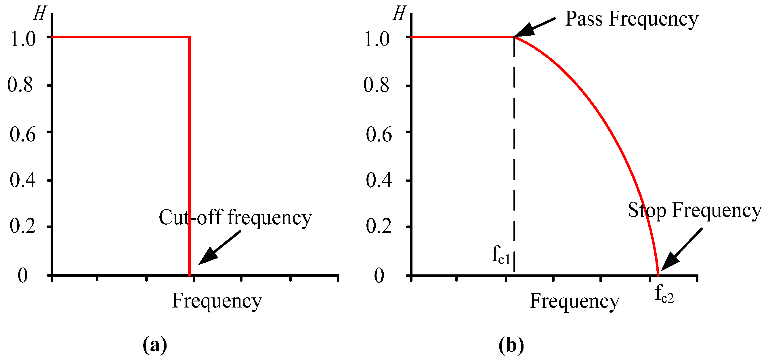
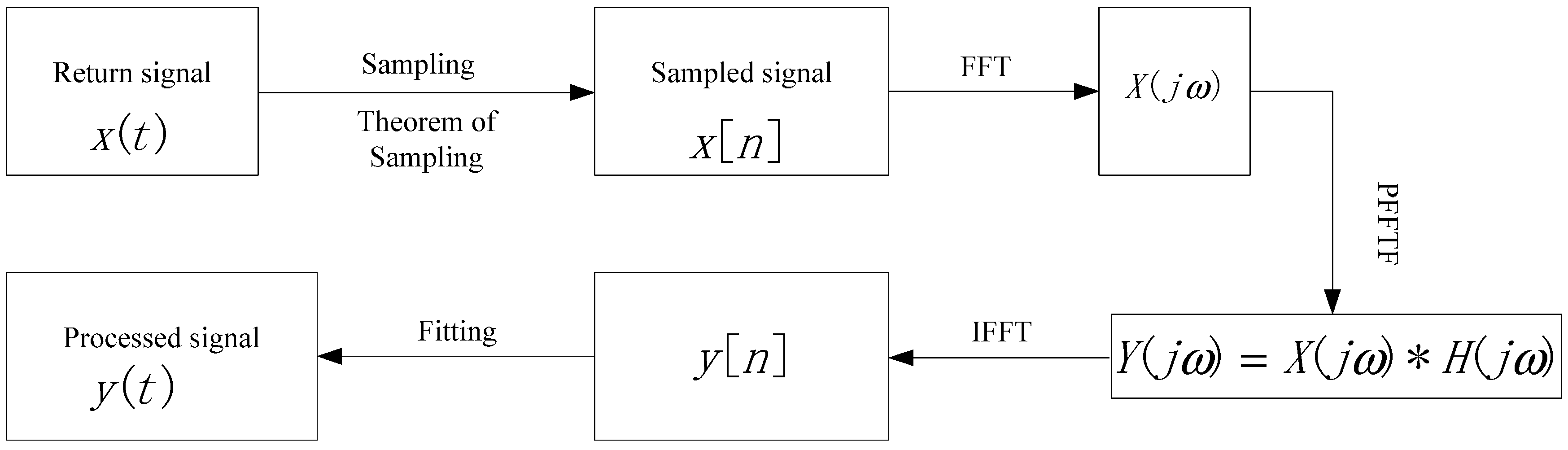
2.1. Theory and Procedure of PFFTF
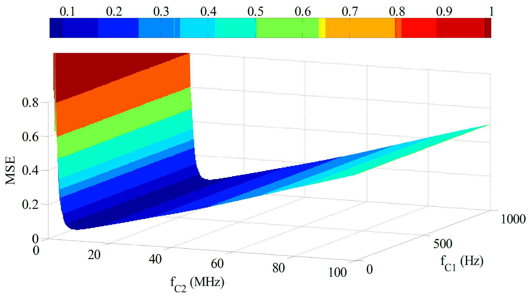
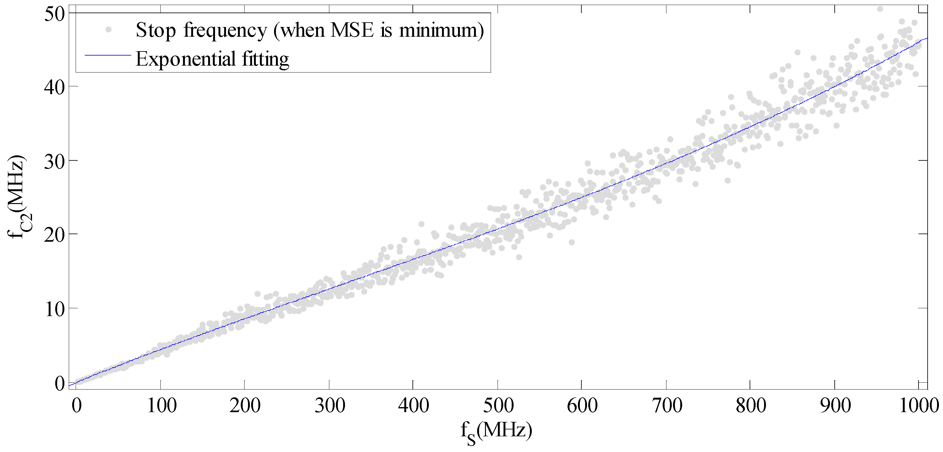

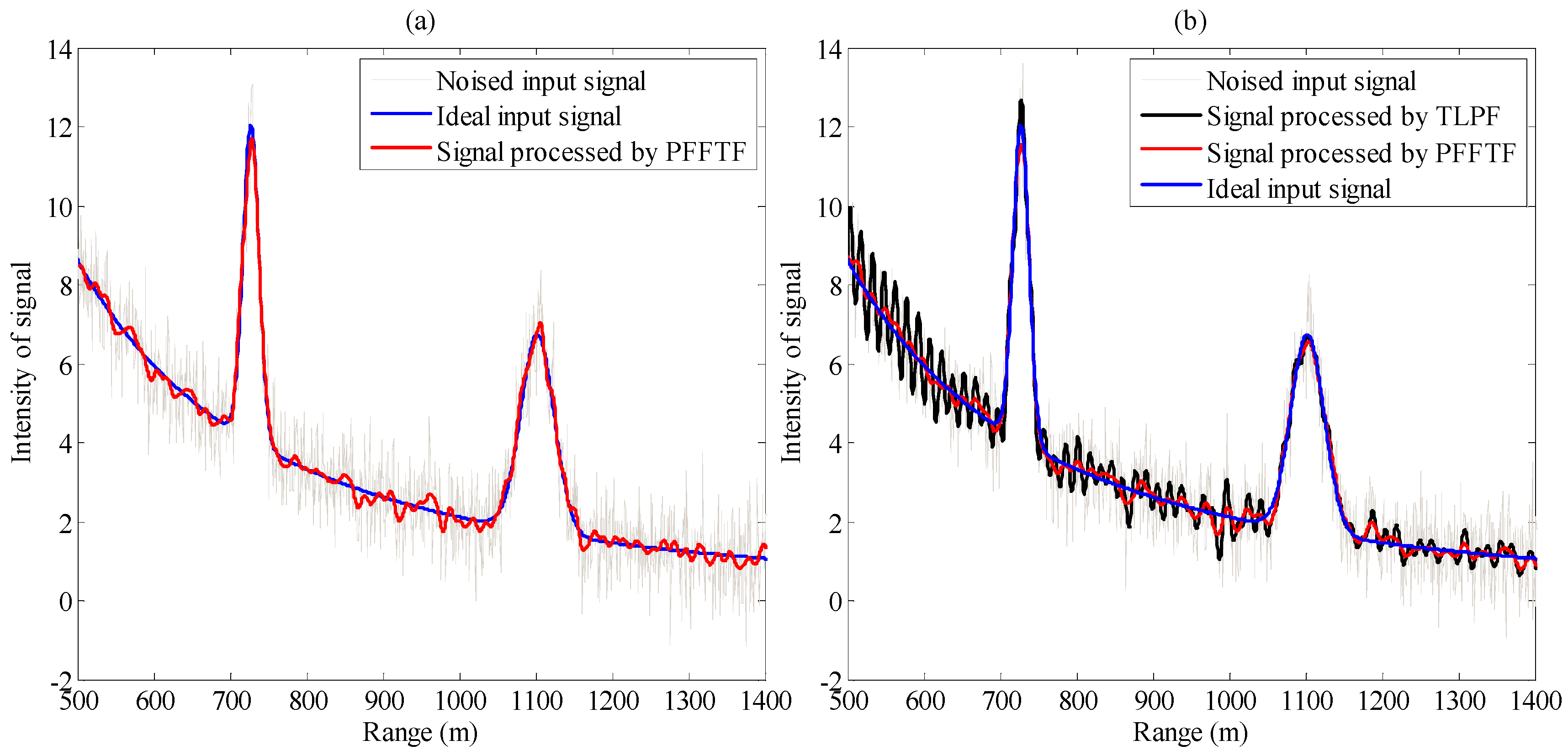
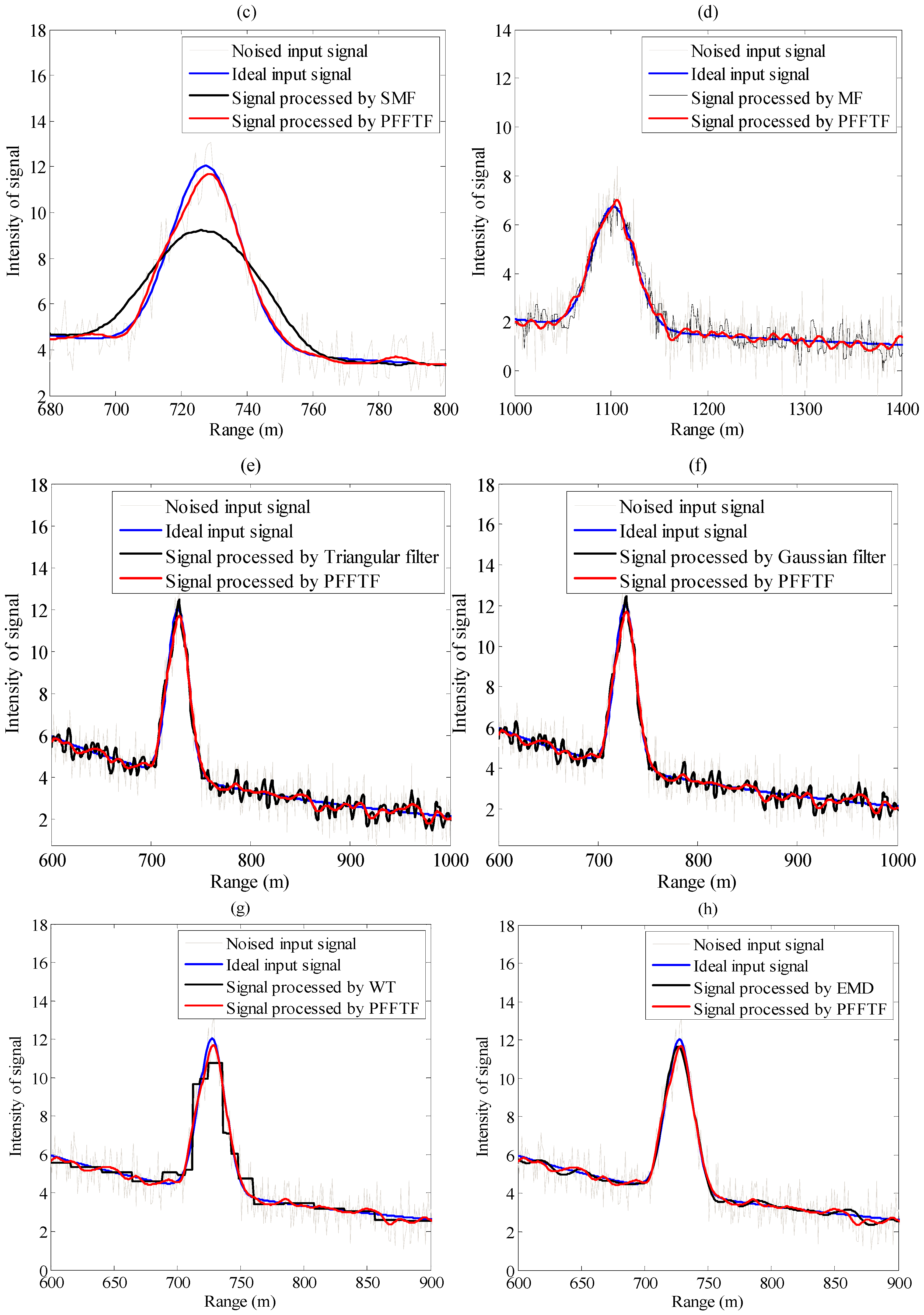
2.2. Simulations

| Method | RSNR_input | RSNR_output | EMSE_input | EMSE_input | Running Time (ms) |
|---|---|---|---|---|---|
| TLPF | 15.4686 | 20.7557 | 0.555 | 0.1644 | 2.237 |
| Triangular | 21.6521 | 0.1425 | 3.233 | ||
| Gaussian | 23.5682 | 0.0985 | 3.512 | ||
| SMF | 18.7609 | 0. 2530 | 2.587 | ||
| MF | 20.9600 | 0.1569 | 2.106 | ||
| WT | 24.0133 | 0.0658 | 200.526 | ||
| EMD | 27.8862 | 0.0321 | 1612.534 | ||
| PFFTF | 27.6606 | 0.0335 | 2.855 |
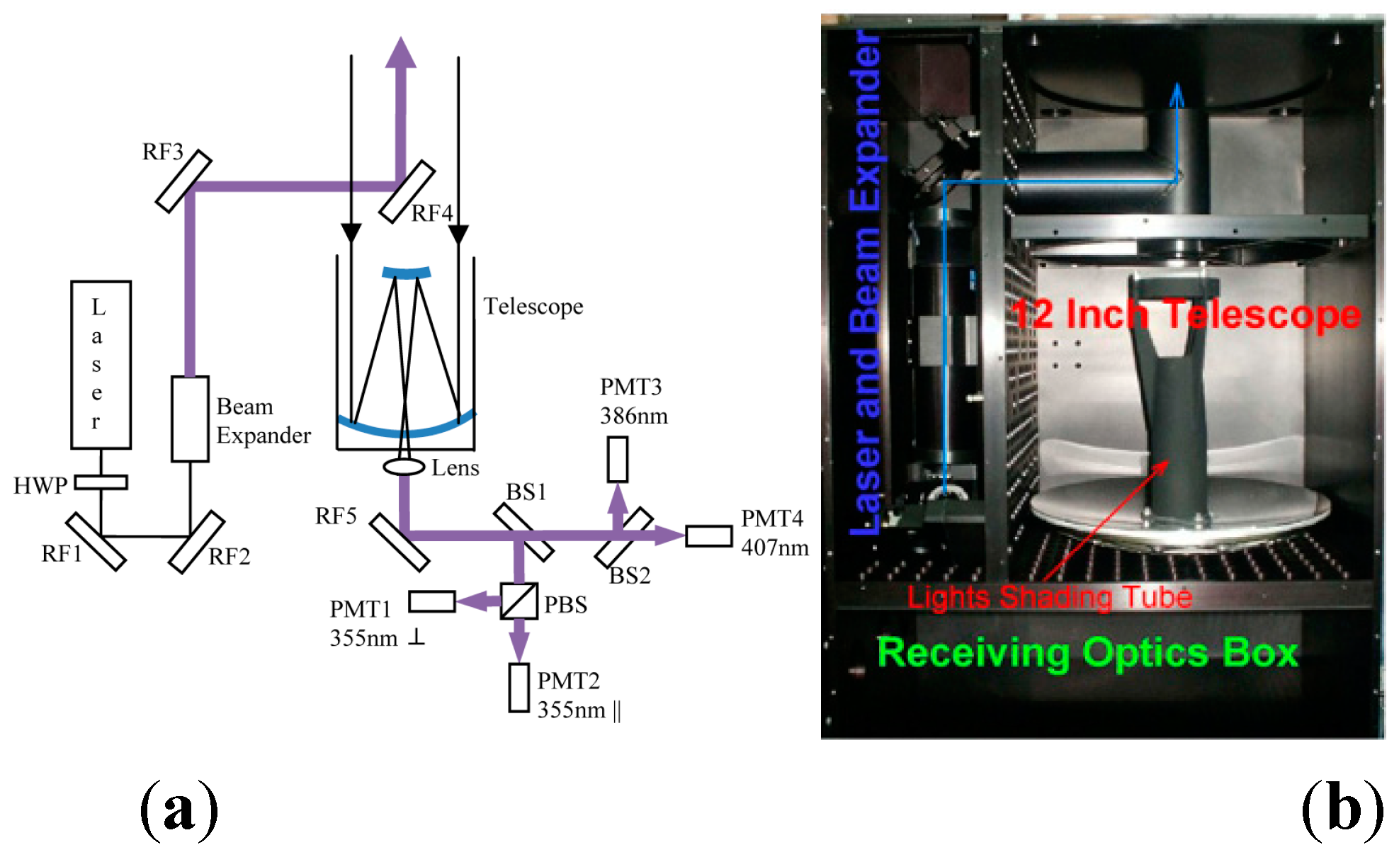
3. Lidar System

| Transmitter | |||
| Laser | Nd:YAG laser (Bigsky CFR400 GRM) | ||
| Wavelength | 354.7 nm | ||
| Pulse energy | 50 mJ | ||
| Pulse width | 7 ns | ||
| Pulse Repetition Frequency (PRF) | 30 Hz | ||
| Beam divergence | 1.8 mrad | ||
| Beam expander | 5X | ||
| Receiver | |||
| Telescope aperture | 12 inch | ||
| Field of View | 1 mard | ||
| Receiving Channels | 4 | ||
| Polarization | Horizontal & Vertical | ||
| Detector | PMT (Hamamatsu H5873) | ||
| Filter center wavelength | 354.7 nm | 386.7 nm | 407.5 nm |
| Filter Bandwidth (FWHM) | 0.3 nm | 0.3 nm | 0.3 nm |
| Data Acquisition System | 12-bit A/D (GAGE) | ||
| Sampling rate | 200 MSPS | ||
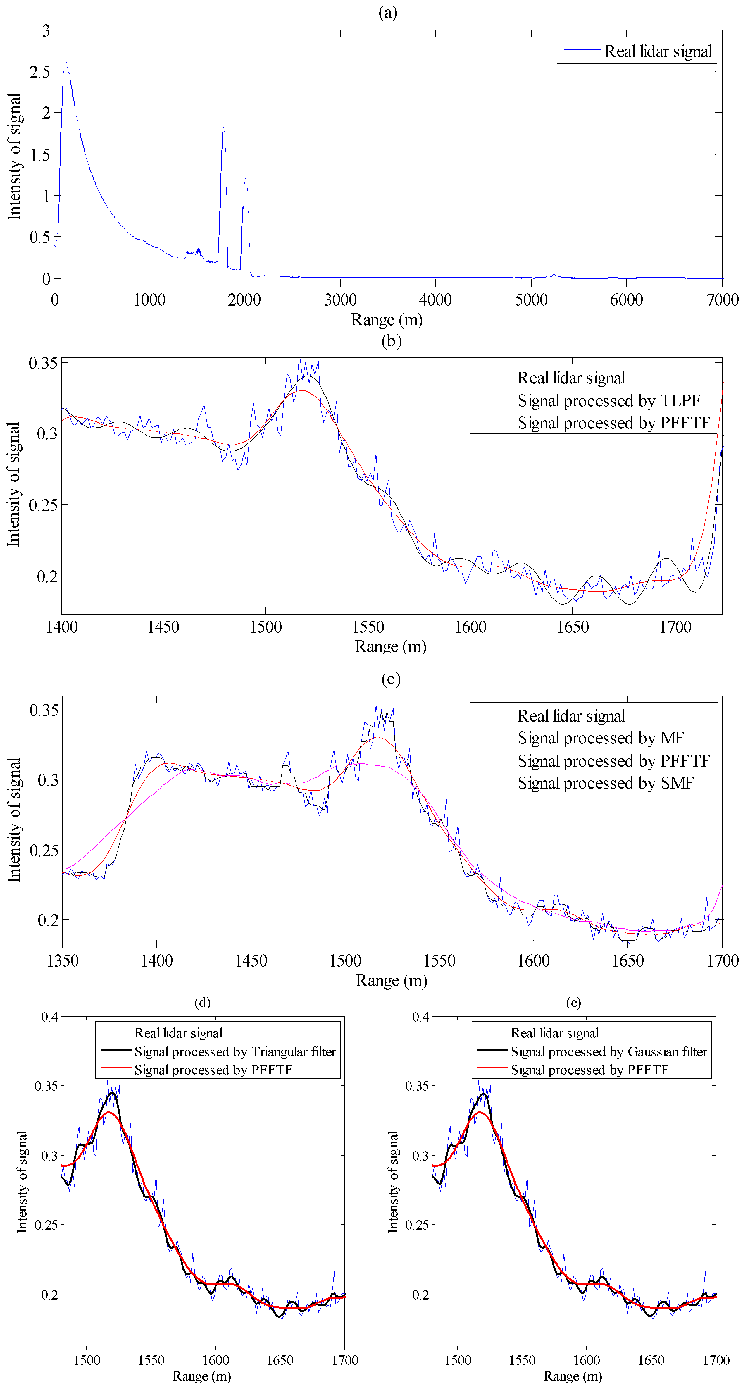
4. Experiments
5. Conclusions
Acknowledgments
Author Contributions
Conflicts of Interest
References
- Ansmann, W.; Riebesell, M.; Weitkamp, C. Measurement of Atmospheric Aerosol Extinction Profiles with a Raman Lidar. Opt. Lett. 1990, 15, 746–748. [Google Scholar] [CrossRef] [PubMed]
- Wu, S.; Liu, Z.; Liu, B. Enhancement of Lidar Backscatters Signal-to-Noise Ratio Using Empirical Mode Decomposition Method. Opt. Commun. 2006, 267, 137–144. [Google Scholar] [CrossRef]
- Liu, B.; Wang, Z. Improved Calibration Method for Depolarization Lidar Measurement. Opt. Express 2013, 21, 14583–14590. [Google Scholar] [CrossRef] [PubMed]
- Tian, P.; Cao, X.; Liang, J.; Zhang, L.; Yi, N.; Wang, L.; Cheng, X. Improved Empirical Mode Decomposition Based Denoising Method for Lidar Signals. Opt. Commun. 2014, 325, 54–59. [Google Scholar] [CrossRef]
- Liu, B.; Wu, D.; Fan, A.; Wang, B.; Yuan, L.; Bo, G.; Zhou, J. Development of a Mobile Raman—Mie Lidar System for All Time Water Vapor and Aerosol Detection. J. Quant. Spectrosc. Radiat. Trans. 2011, 112, 230–235. [Google Scholar] [CrossRef]
- Huang, B.N.E.; Shen, Z.; Long, S.R.; Wu, M.C.; Shih, H.H. The Empirical Mode Decomposition and the Hilbert Spectrum for Nonlinear and Non-Stationary Time Series Analysis. Proc. R. Soc. Lond. A 1998, 454, 903–995. [Google Scholar] [CrossRef]
- Fang, H.; Huang, D. Noise Reduction in Lidar Signal Based on Discrete Wavelet Transform. Opt. Commun. 2004, 233, 67–76. [Google Scholar] [CrossRef]
- Kedzierski, M.; Fryskowska, A. Terrestrial and Aerial Laser Scanning Data Integration Using Wavelet Analysis for the Purpose of 3D Building Modeling. Sensors 2014, 14, 12070–12092. [Google Scholar] [CrossRef] [PubMed]
- Whiteman, D.N.; Melfi, S.H.; Ferrare, R.A. Raman Lidar System for the Measurement of Water Vapor and Aerosols in the Earth’s Atmosphere. Appl. Opt. 1992, 31, 3068–3082. [Google Scholar] [CrossRef] [PubMed]
- Liu, B.; Wang, Z.; Cai, Y.; Wechsler, P.; Kuestner, W.; Burkhart, M.; Welch, W. Compact Airborne Raman Lidar for Profiling Aerosol, Water Vapor and Clouds. Opt. Express 2014, 22, 20613–20621. [Google Scholar] [CrossRef] [PubMed]
- Liu, Z.; Zhang, N.; Wang, R.; Zhu, J. Doppler Wind Lidar Data Acquisition System and Data Analysis by Empirical Mode Decomposition Method. Opt. Eng. 2007, 46, 026001–026008. [Google Scholar] [CrossRef]
- Hook, J. Smoothing Non-Smooth Systems with Low-Pass Filters. Phys. D. Nonlinear Phenom. 2014, 269, 76–85. [Google Scholar] [CrossRef]
- Whiteman, D.N. Examination of the Traditional Raman Lidar Technique. I. Evaluating the Temperature-Dependent Lidar Equations. Appl. Opt. 2003, 42, 2571–2592. [Google Scholar] [CrossRef] [PubMed]
- Ansmann, A.; Wandinger, U.; Riebesell, M.; Weitkamp, C.; Michaelis, W. Independent Measurement of the Extinction and Backscatter Profiles in Cirrus Clouds by Using a Combined Raman Elastic-Backscatter Lidar. Appl. Opt. 1992, 31, 7113–7131. [Google Scholar] [CrossRef] [PubMed]
© 2015 by the authors; licensee MDPI, Basel, Switzerland. This article is an open access article distributed under the terms and conditions of the Creative Commons Attribution license (http://creativecommons.org/licenses/by/4.0/).
Share and Cite
Jiao, Z.; Liu, B.; Liu, E.; Yue, Y. Low-Pass Parabolic FFT Filter for Airborne and Satellite Lidar Signal Processing. Sensors 2015, 15, 26085-26095. https://doi.org/10.3390/s151026085
Jiao Z, Liu B, Liu E, Yue Y. Low-Pass Parabolic FFT Filter for Airborne and Satellite Lidar Signal Processing. Sensors. 2015; 15(10):26085-26095. https://doi.org/10.3390/s151026085
Chicago/Turabian StyleJiao, Zhongke, Bo Liu, Enhai Liu, and Yongjian Yue. 2015. "Low-Pass Parabolic FFT Filter for Airborne and Satellite Lidar Signal Processing" Sensors 15, no. 10: 26085-26095. https://doi.org/10.3390/s151026085
APA StyleJiao, Z., Liu, B., Liu, E., & Yue, Y. (2015). Low-Pass Parabolic FFT Filter for Airborne and Satellite Lidar Signal Processing. Sensors, 15(10), 26085-26095. https://doi.org/10.3390/s151026085