
A Novel Robot Visual Homing Method Based on SIFT Features

Abstract
:1. Introduction
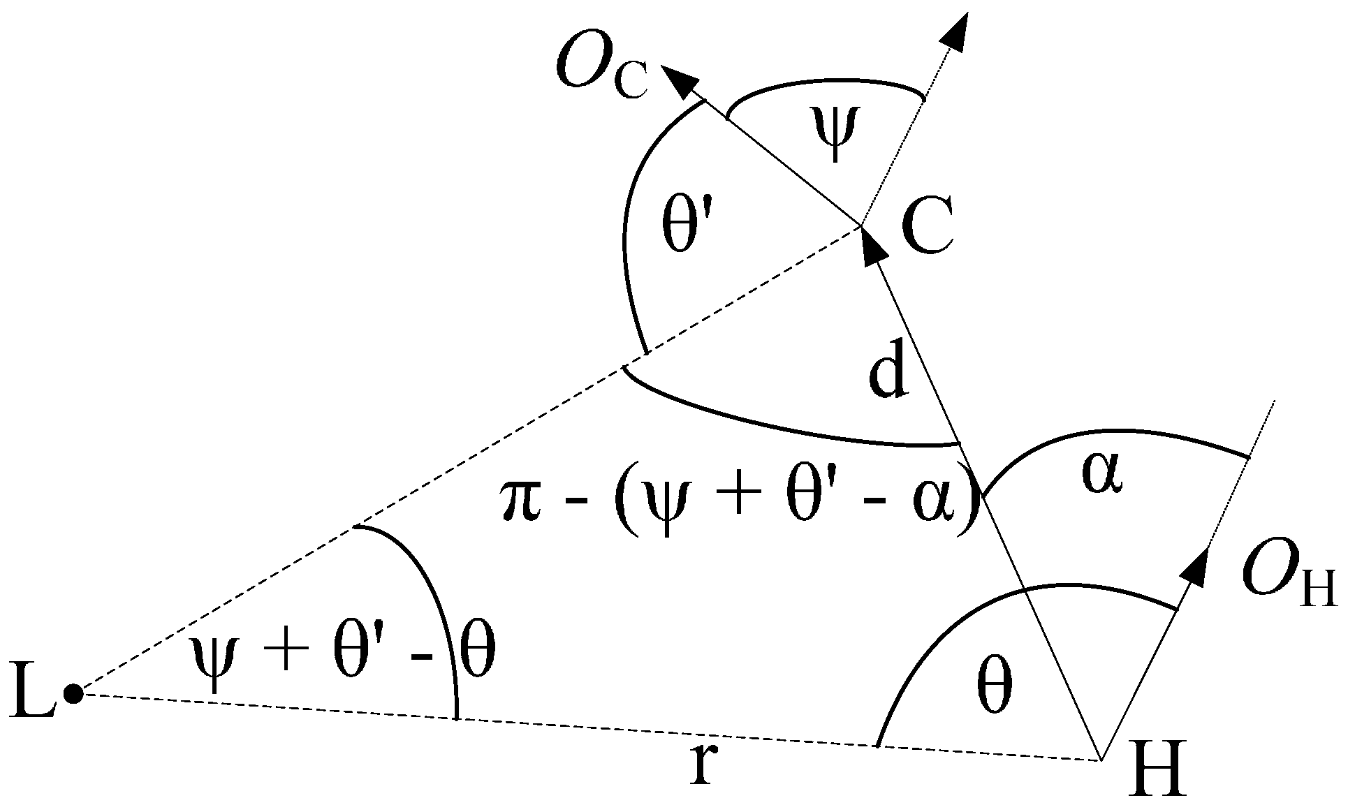
2. Homing Algorithm

3. Landmark Optimization and Overview of the Proposed Method
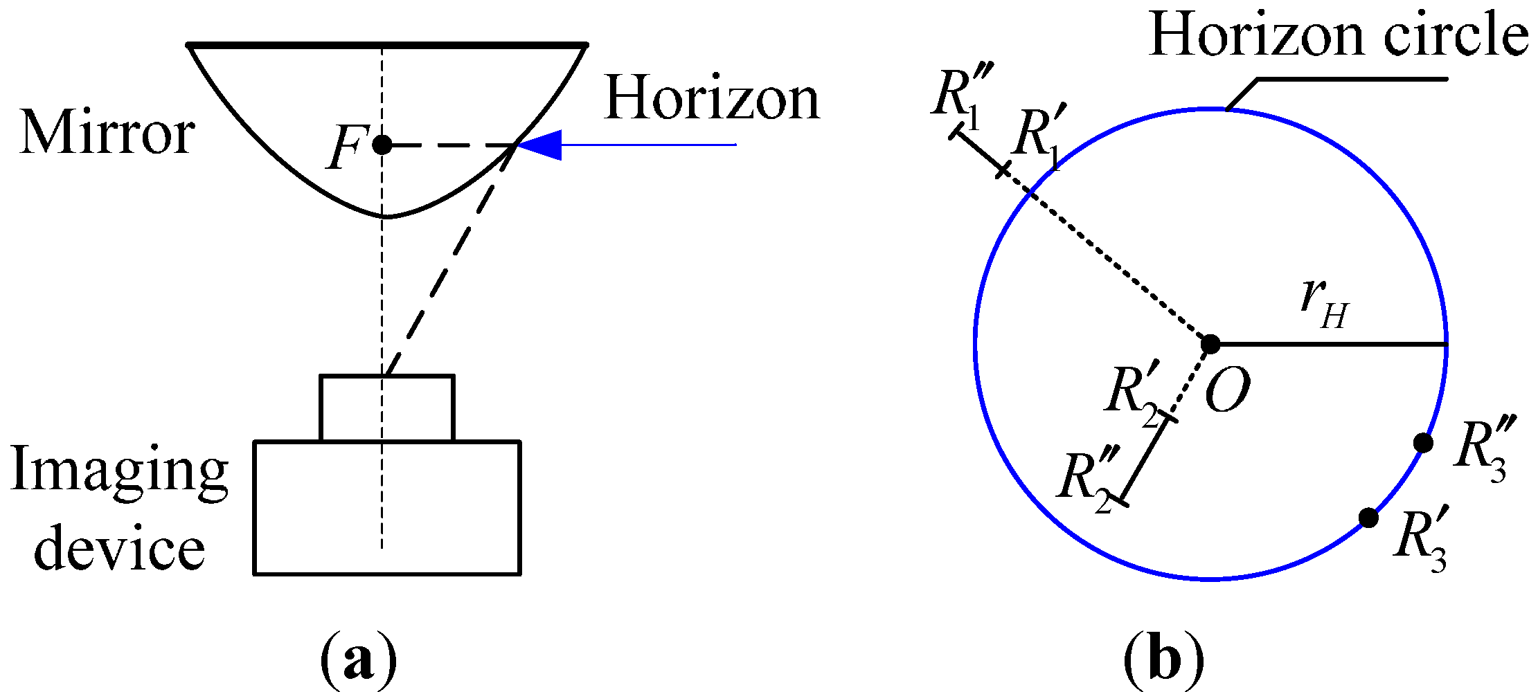
3.1. Landmark Selection
3.2. Mismatching Elimination
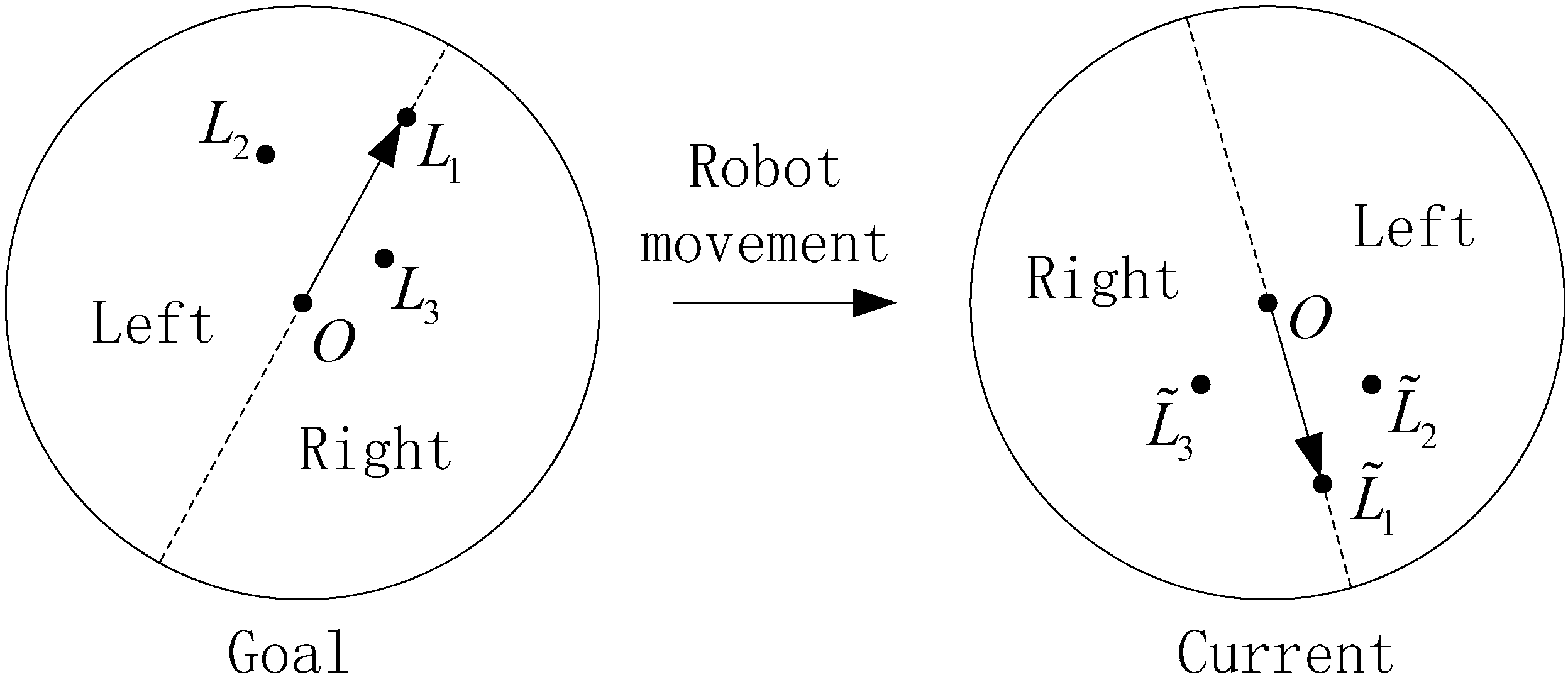
3.2.1. Two Distribution Constraints
3.2.2. Mismatching Elimination Algorithm

3.3. Overview of the Proposed Visual Homing Method

4. Experiments
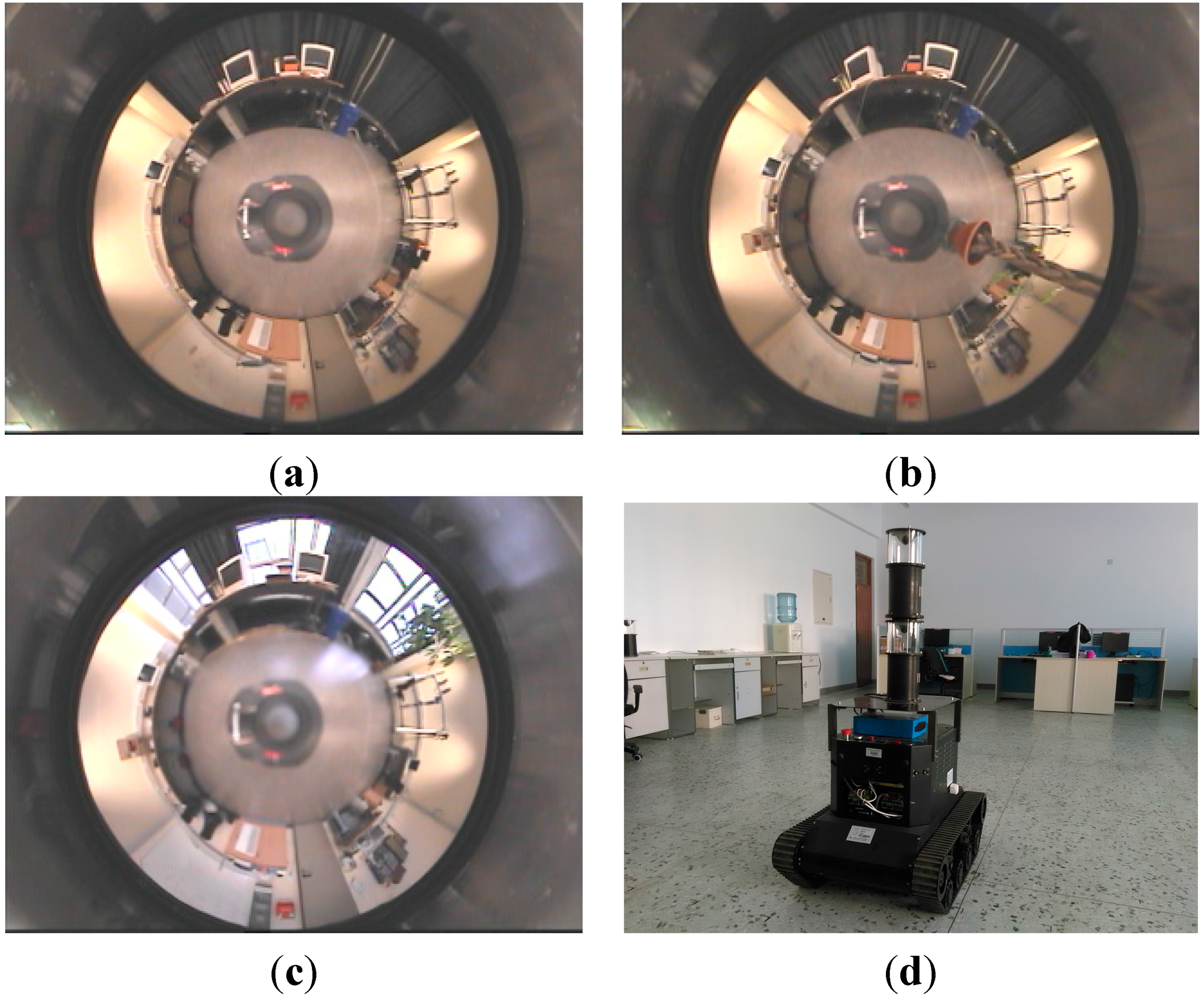
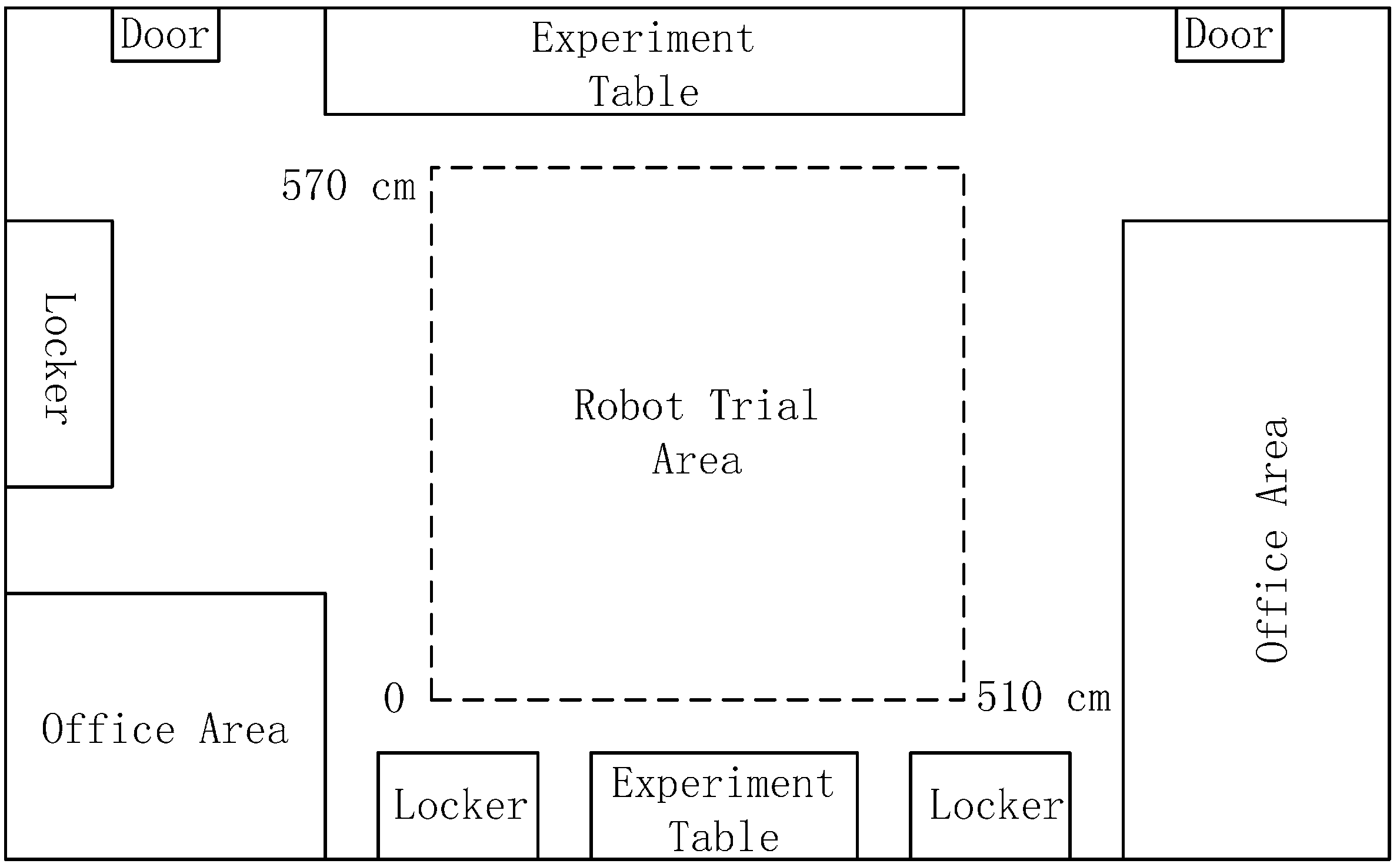
4.1. Image Databases and Robot Platform

4.2. Parameter Settings for Experiments

| Parameters | Value | Parameters | Value |
|---|---|---|---|
| S | 5 | αW | [0, 355]/72/5 |
| TDOG | 0.04/S | nR | 5 |
| ρW | [0, 0.95]/20/0.05 | VTH | 4 |
| ψW | [0, 355]/72/5 |
| Method | Average Computation Time (s) | ||
|---|---|---|---|
| original | arboreal | day | |
| Warping | 21.051 | 18.643 | 19.541 |
| Proposed | 14.559 | 12.638 | 13.854 |
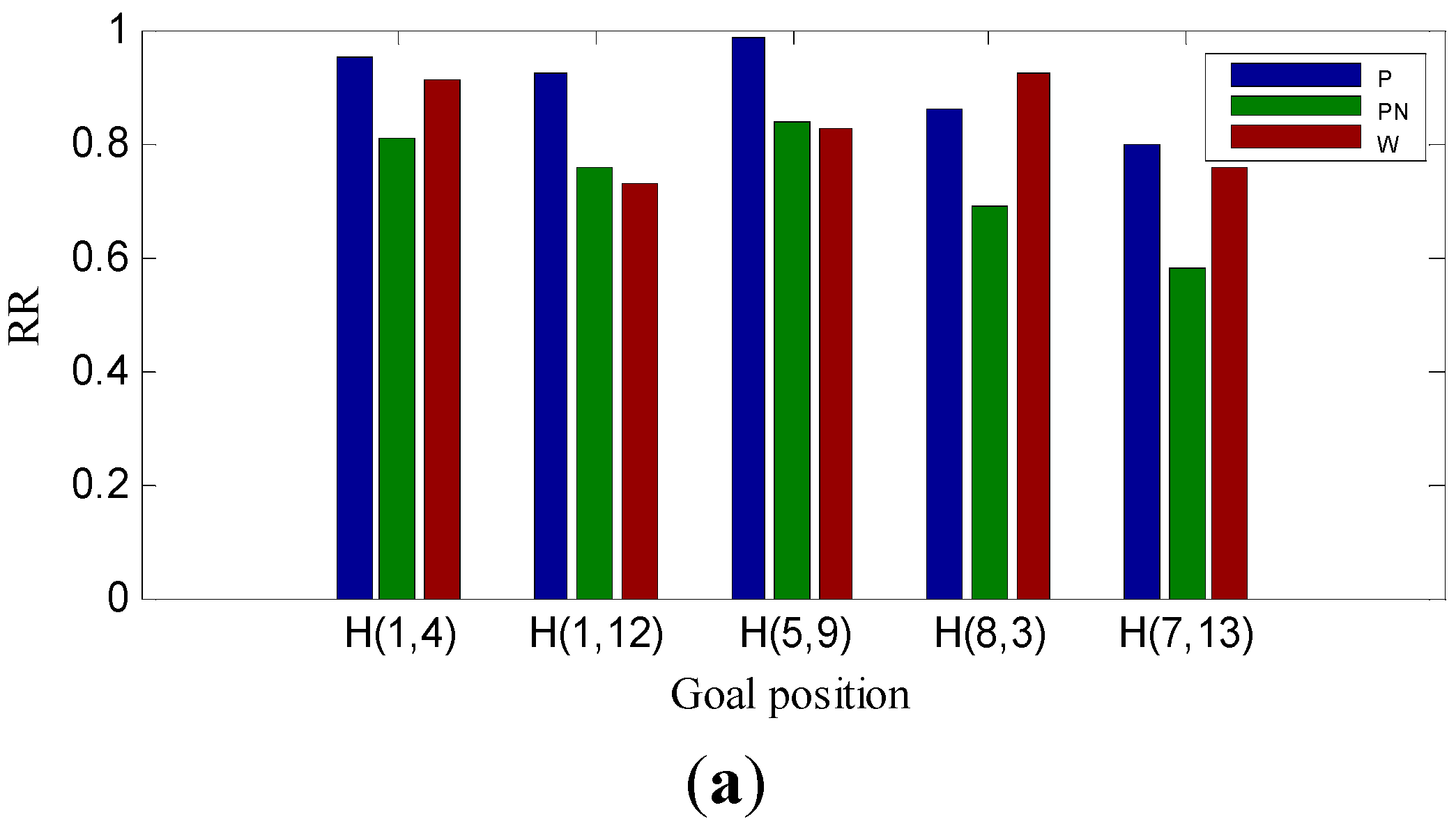
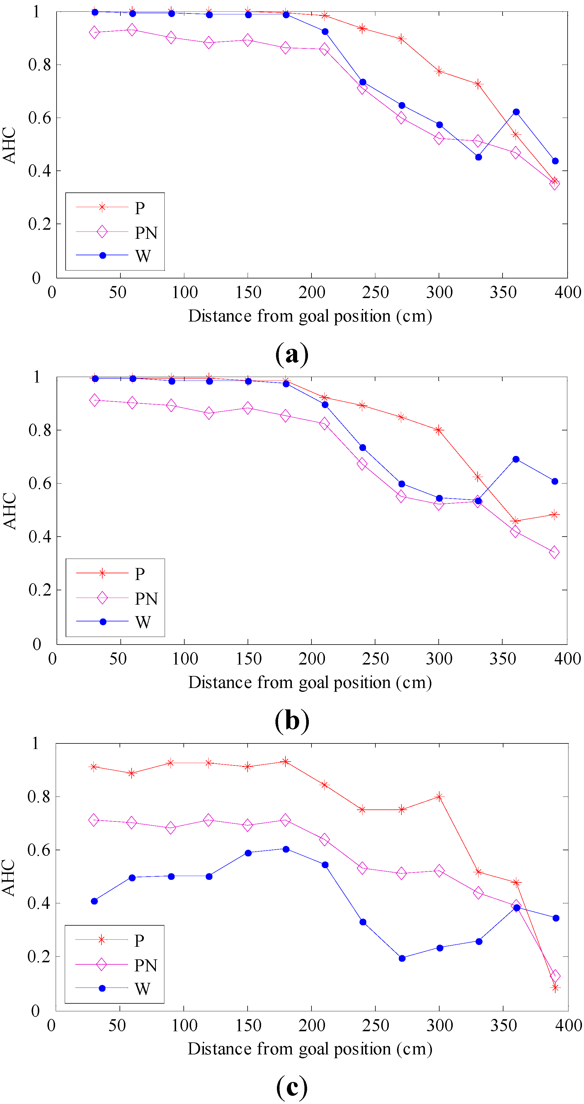
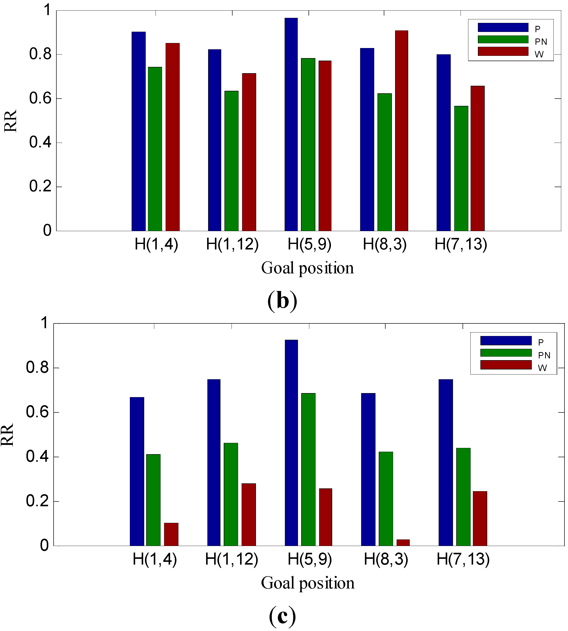
4.3. Performance Metrics
- Step 1: The robot moves a step according to the corresponding βh(x,y).
- Step 2: If the following two cases happen, jump to Step 4.
- Case 1: The robot arrives at the goal position H.
- Case 2: The robot travels a distance longer than half of the perimeter of the capture grid.
- Step 3: Continue to perform Step 1.
- Step 4: If Case 1 happens, the homing trial is successful; if Case 1 does not happen and Case 2 happens, the trial has failed.
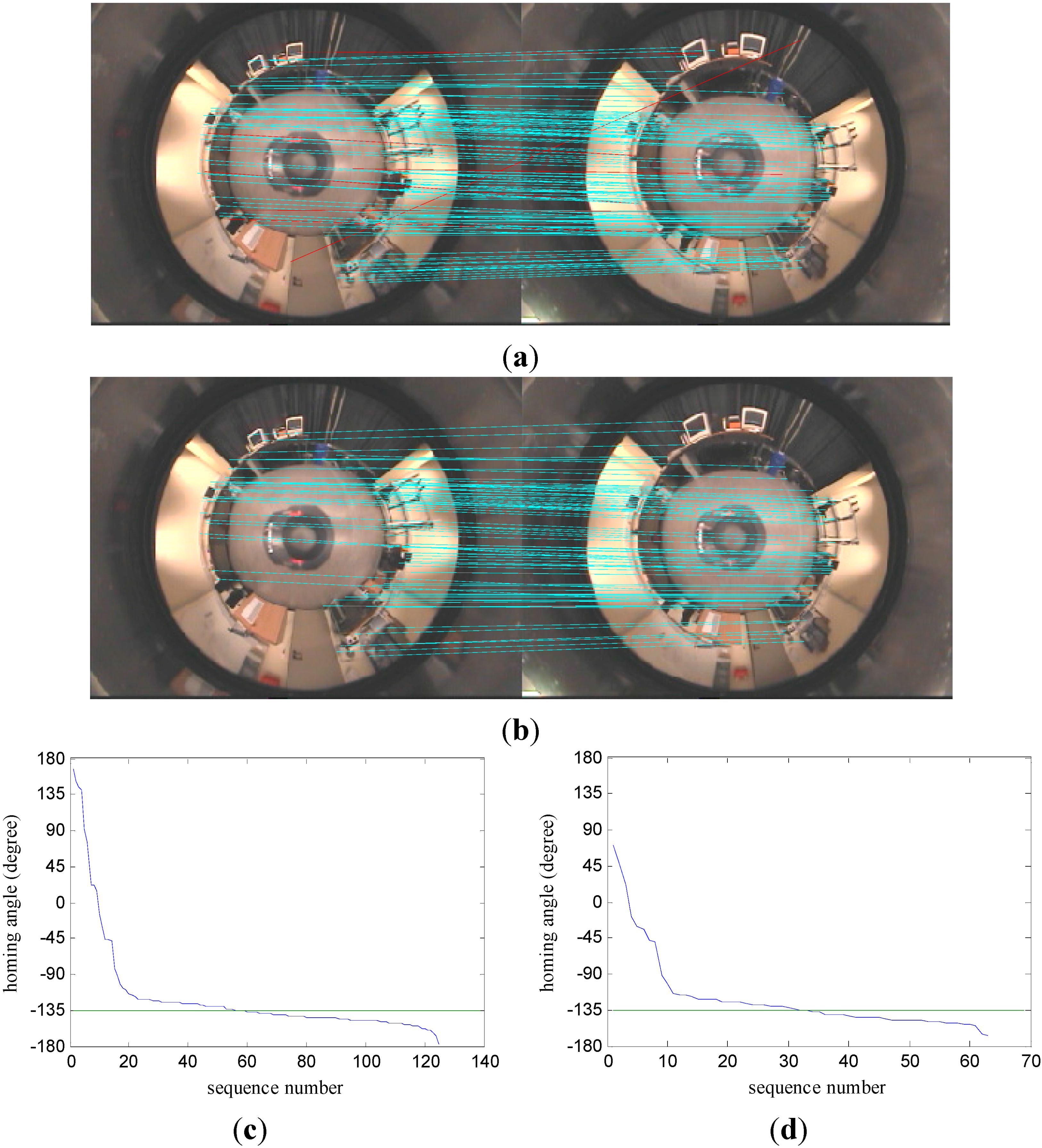
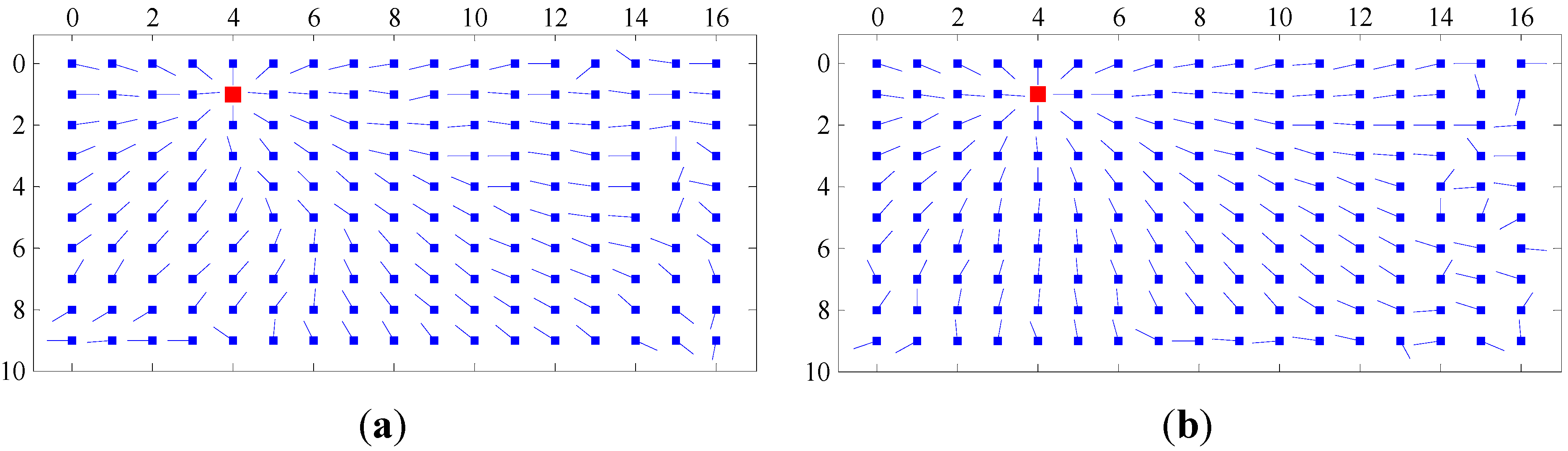
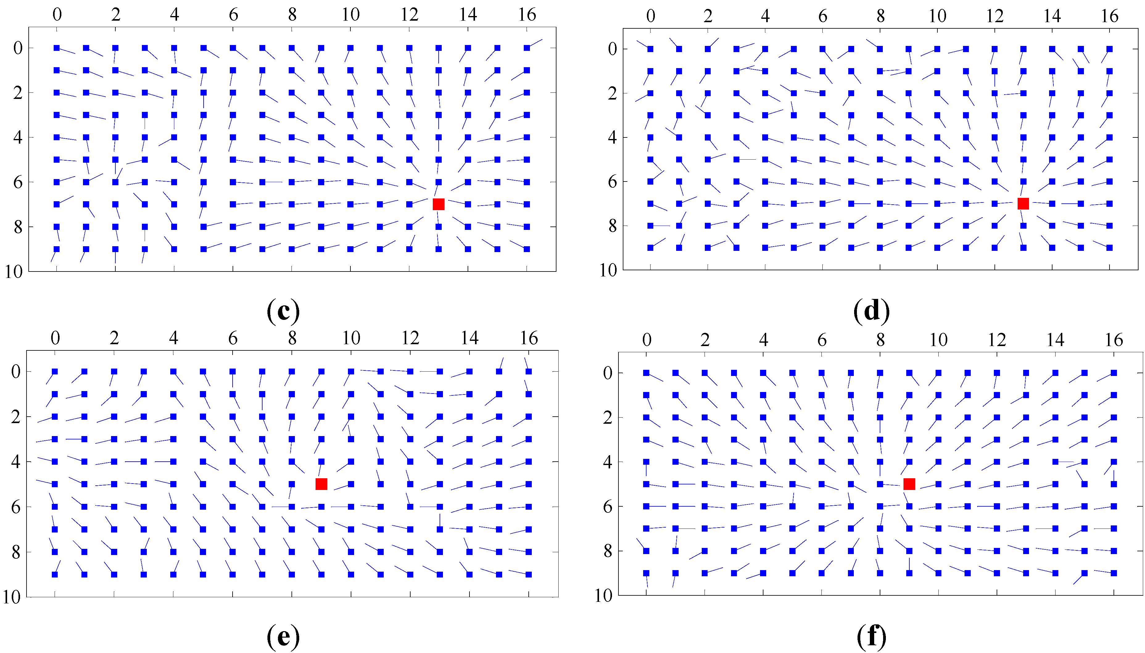
4.4. Homing Experiments on Image Databases


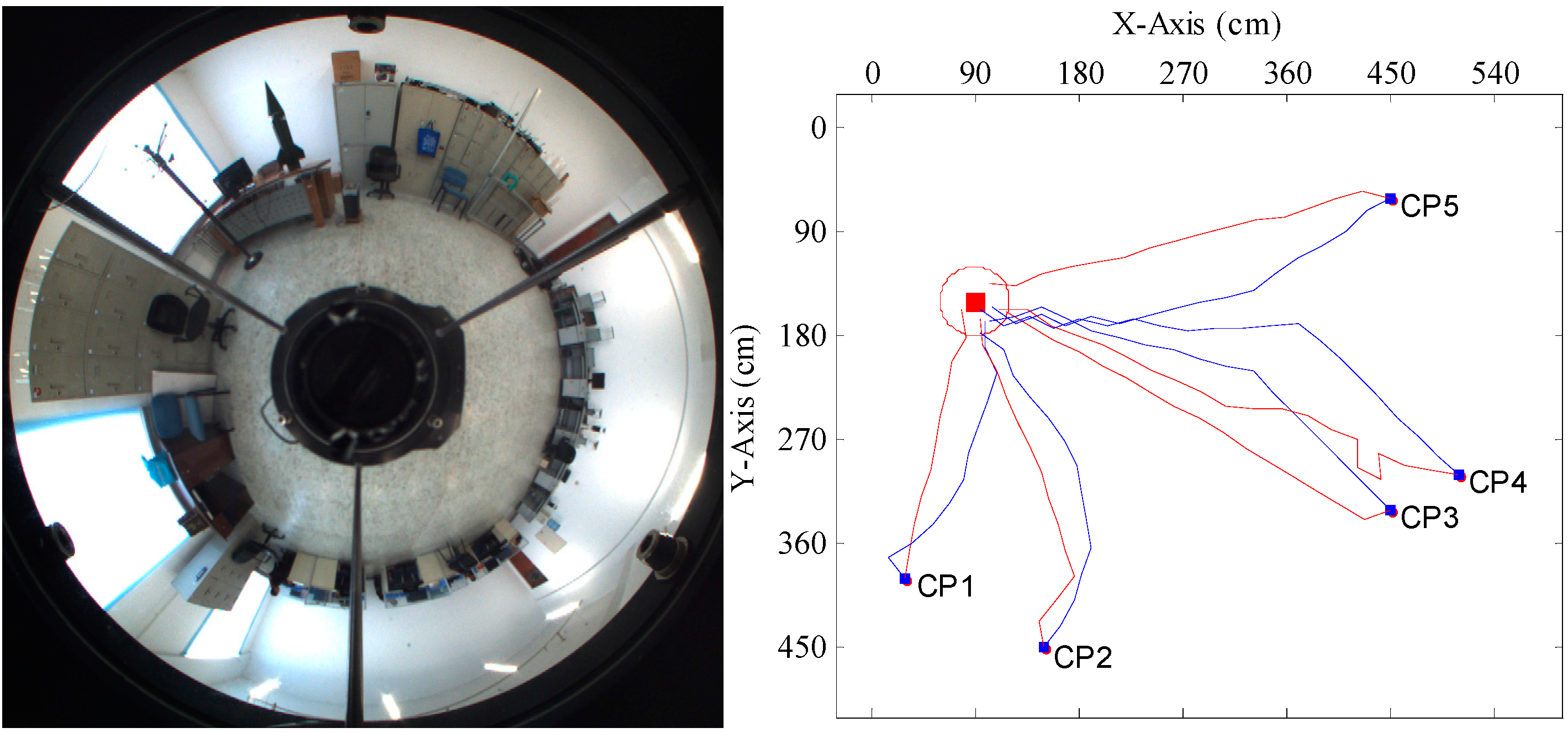
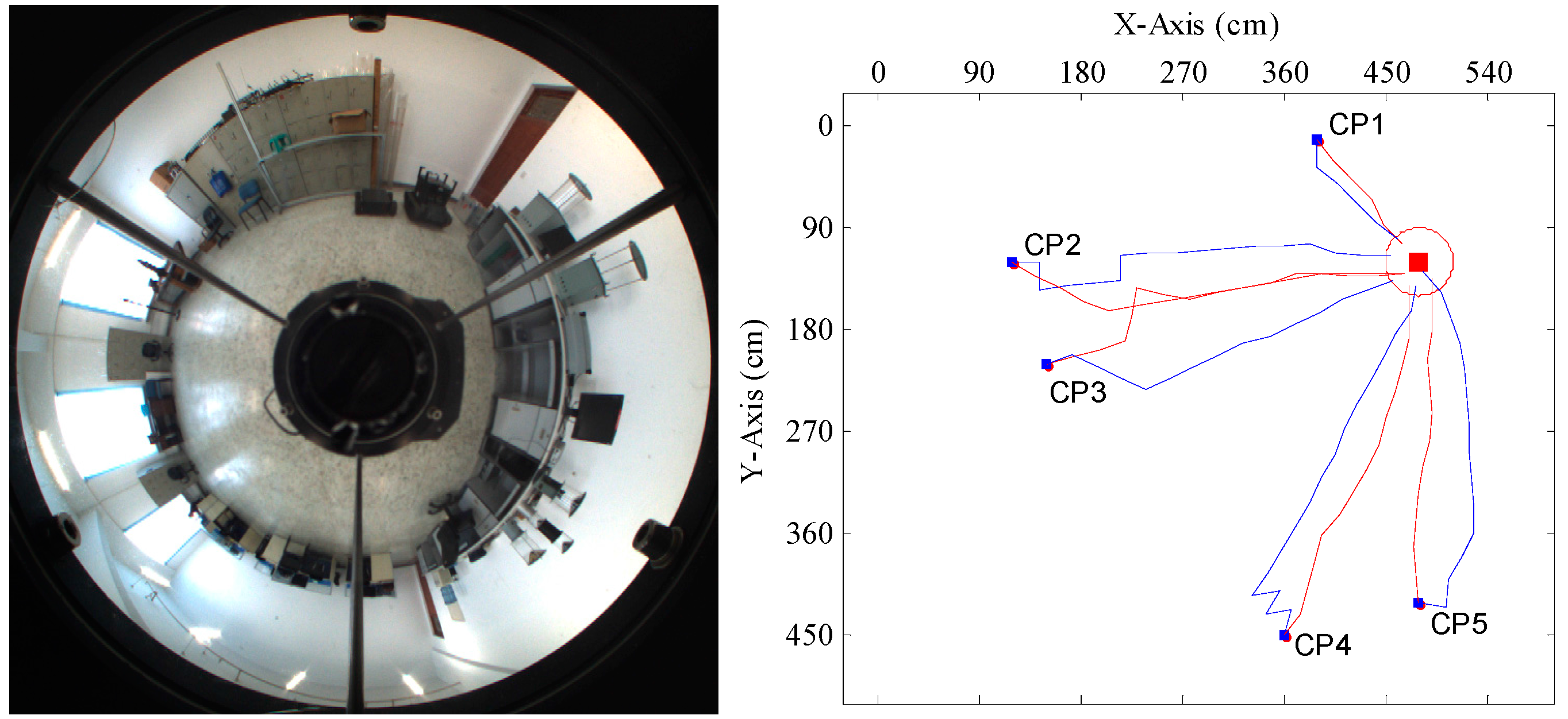
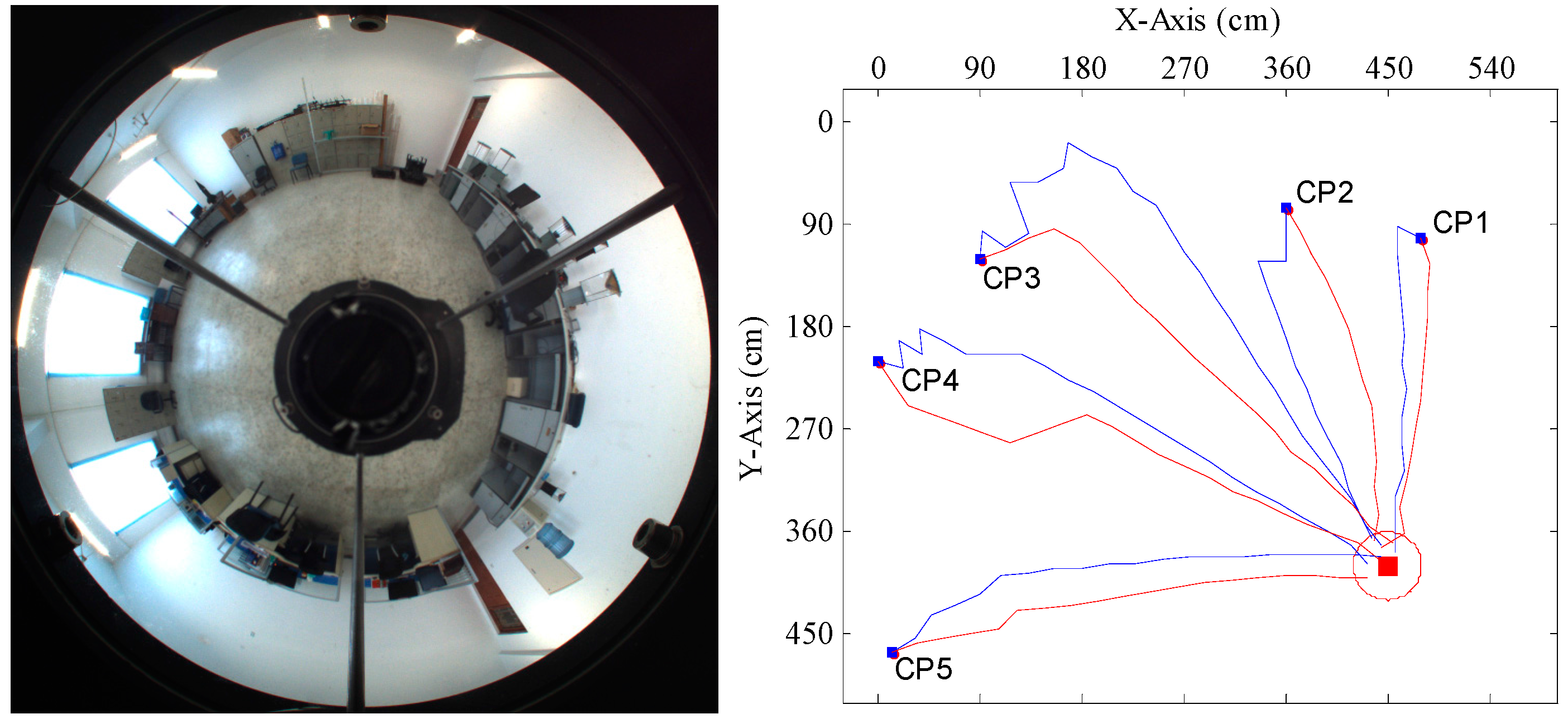
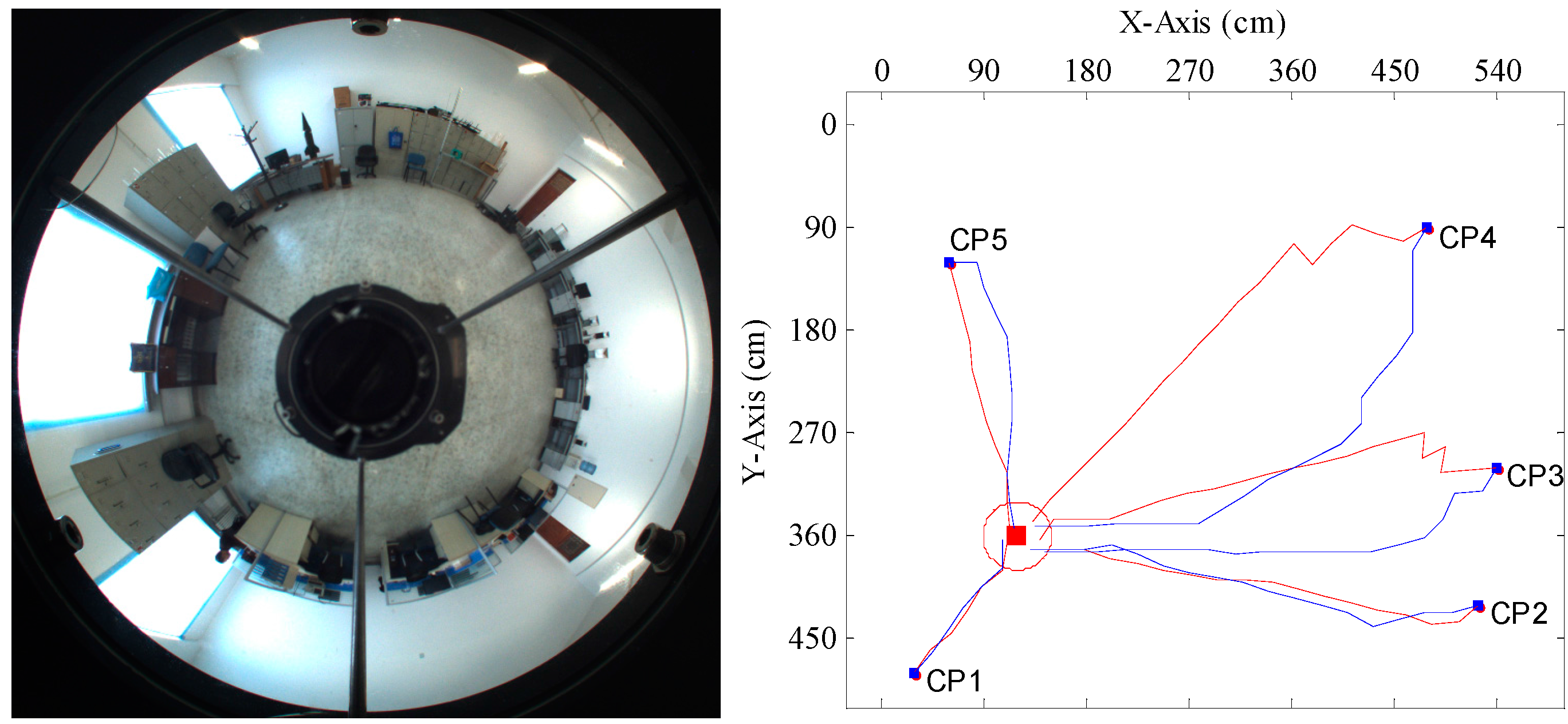
4.5. Homing Trials in a Real Scene

| Method | CP1 | CP2 | CP3 | CP4 | CP5 | |||||
|---|---|---|---|---|---|---|---|---|---|---|
| N | σ | N | σ | N | σ | N | σ | N | σ | |
| Warping | 11 | 24.54 | 13 | 21.12 | 17 | 15.03 | 20 | 19.14 | 16 | 18.78 |
| Proposed | 10 | 6.34 | 13 | 11.57 | 16 | 5.81 | 20 | 15.43 | 15 | 6.47 |

| Method | CP1 | CP2 | CP3 | CP4 | CP5 | |||||
|---|---|---|---|---|---|---|---|---|---|---|
| N | σ | N | σ | N | σ | N | σ | N | σ | |
| Warping | 5 | 9.66 | 16 | 15.23 | 14 | 11.79 | 17 | 19.09 | 14 | 20.19 |
| Proposed | 5 | 6.47 | 15 | 11.42 | 15 | 14.92 | 14 | 9.29 | 12 | 8.31 |
| Method | CP1 | CP2 | CP3 | CP4 | CP5 | |||||
|---|---|---|---|---|---|---|---|---|---|---|
| N | σ | N | σ | N | σ | N | σ | N | σ | |
| Warping | 6 | 8.01 | 17 | 10.65 | 18 | 14.79 | 21 | 23.82 | 11 | 13.89 |
| Proposed | 6 | 8.13 | 17 | 8.07 | 20 | 16.24 | 20 | 11.89 | 10 | 5.10 |

| Method | CP1 | CP2 | CP3 | CP4 | CP5 | |||||
|---|---|---|---|---|---|---|---|---|---|---|
| N | σ | N | σ | N | σ | N | σ | N | σ | |
| Warping | 13 | 15.13 | 14 | 12.93 | 27 | 31.89 | 23 | 15.99 | 19 | 12.14 |
| Proposed | 12 | 9.50 | 13 | 9.89 | 20 | 15.22 | 21 | 11.32 | 18 | 5.29 |
5. Conclusions
Acknowledgments
Author Contributions
Conflicts of Interest
References
- López-Nicolás, G.; Guerrero, J.J.; Sagüés, C. Multiple homographies with omnidirectional vision for robot homing. Robot. Auton. Syst. 2010, 58, 773–783. [Google Scholar] [CrossRef]
- Ohnishi, N.; Imiya, A. Appearance-based navigation and homing for autonomous mobile robot. Image Vis. Comput. 2013, 31, 511–532. [Google Scholar] [CrossRef]
- Aranda, M.; López-Nicolás, G.; Sagüés, C. Angle-based homing from a reference image set using the 1D trifocal tensor. Auton. Robot. 2013, 34, 73–91. [Google Scholar] [CrossRef]
- Labrosse, F. Short and long-range visual navigation using warped panoramic images. Robot. Auton. Syst. 2007, 55, 675–684. [Google Scholar] [CrossRef]
- Baddeley, B.; Graham, P.; Philippides, A.; Husbands, P. Holistic visual encoding of ant-like routes: Navigation without waypoints. Adapt. Behav. 2011, 19, 3–15. [Google Scholar] [CrossRef]
- Yu, S.E.; Lee, C.; Kim, D. Analyzing the effect of landmark vectors in homing navigation. Adapt. Behav. 2012, 20, 337–359. [Google Scholar] [CrossRef]
- Fu, Y.; Hsiang, T.R. A fast robot homing approach using sparse image waypoints. Image Vis. Comput. 2012, 30, 109–121. [Google Scholar] [CrossRef]
- Liu, M.; Pradalier, C.; Pomerleau, F.; Siegwart, R. Scale-only visual homing from an omnidirectional camera. In Proceedings of the IEEE International Conference on Robotics and Automation, St Paul, MN, USA, 14–18 May 2012; pp. 3944–3949.
- Möller, R.; Krzykawski, M.; Gerstmayr-Hillen, L.; Horst, M.; Fleer, D.; de Jong, J. Cleaning robot navigation using panoramic views and particle clouds as landmarks. Robot. Auton. Syst. 2013, 61, 1415–1439. [Google Scholar] [CrossRef]
- Liu, M.; Pradalier, C.; Siegwart, R. Visual homing from scale with an uncalibrated omnidirectional camera. IEEE Trans. Robot. 2013, 29, 1353–1365. [Google Scholar] [CrossRef]
- Guzel, M.S.; Bicker, R. A behaviour-based architecture for mapless navigation using vision. Int. J. Adv. Robot. Syst. 2012, 9, 18:1–18:13. [Google Scholar]
- Qidan, Z.; Xue, L.; Chengtao, C. Feature optimization for long-range visual homing in changing environments. Sensors 2014, 14, 3342–3361. [Google Scholar]
- Möller, R.; Krzykawski, M.; Gerstmayr, L. Three 2D-warping schemes for visual robot navigation. Auton. Robot. 2010, 29, 253–291. [Google Scholar] [CrossRef]
- Zeil, J.; Hofmann, M.I.; Chahl, J.S. Catchment areas of panoramic snapshots in outdoor scenes. J. Opt. Soc. Am. A Opt. Image Sci. Vis. 2003, 20, 450–469. [Google Scholar] [CrossRef] [PubMed]
- Sturzl, W.; Zeil, J. Depth, contrast and view-based homing in outdoor scenes. Biol. Cybern. 2007, 96, 519–531. [Google Scholar] [CrossRef] [PubMed]
- Arena, P.; De Fiore, S.; Fortuna, L.; Nicolosi, L.; Patane, L.; Vagliasindi, G. Visual homing: experimental results on an autonomous robot. In Proceedings of the European Conference on Circuit Theory and Design, Univ Sevilla, Seville, Spain, 26–30 August 2007; pp. 304–307.
- Möller, R. A model of ant navigation based on visual prediction. J. Theor. Biol. 2012, 305, 118–130. [Google Scholar] [CrossRef] [PubMed]
- Churchill, D.; Vardy, A. An orientation invariant visual homing algorithm. J. Intell. Robot. Syst. 2013, 71, 3–29. [Google Scholar] [CrossRef]
- Vardy, A.; Möller, R. Biologically plausible visual homing methods based on optical flow techniques. Connect. Sci. 2005, 17, 47–89. [Google Scholar] [CrossRef]
- Briggs, A.J.; Detweiler, C.; Li, Y.; Mullen, P.C.; Scharstein, D. Matching scale-space features in 1D panoramas. Comput. Vis. Image Underst. 2006, 103, 184–195. [Google Scholar] [CrossRef]
- Loizou, S.G.; Kumar, V. Biologically inspired bearing-only navigation and tracking. In Proceedings of the IEEE Conference on Decision and Control, New Orleans, LA, USA, 12–14 December 2007; pp. 6121–6126.
- Liu, M.; Pradalier, C.; Chen, Q.J.; Siegwart, R. A bearing-only 2D/3D-homing method under a visual servoing framework. In Proceedings of the IEEE International Conference on Robotics and Automation, Anchorage, AK, USA, 3–8 May 2010; pp. 4062–4067.
- Möller, R.; Vardy, A. Local visual homing by matched-filter descent in image distances. Biol. Cybern. 2006, 95, 413–430. [Google Scholar] [CrossRef] [PubMed]
- Möller, R.; Vardy, A.; Kreft, S.; Ruwisch, S. Visual homing in environments with anisotropic landmark distribution. Auton. Robot. 2007, 23, 231–245. [Google Scholar] [CrossRef]
- Lambrinos, D.; Möller, R.; Labhart, T.; Pfeifer, R.; Wehner, R. A mobile robot employing insect strategies for navigation. Robot. Auton. Syst. 2000, 30, 39–64. [Google Scholar] [CrossRef]
- Basten, K.; Mallot, H.A. Simulated visual homing in desert ant natural environments: Efficiency of skyline cues. Biol. Cybern. 2010, 102, 413–425. [Google Scholar] [CrossRef] [PubMed]
- Ramisa, A.; Goldhoom, A.; Aldavert, D.; Toledo, R.; de Mantaras, R.L. Combining invariant features and the ALV homing method for autonomous robot navigation based on panoramas. J. Intell. Robot. Syst. 2011, 64, 625–649. [Google Scholar] [CrossRef]
- Franz, M.O.; Schölkopf, B.; Mallot, H.A.; Bülthoff, H.H. Where did I take that snapshot? Scene-based homing by image matching. Biol. Cybern. 1998, 79, 191–202. [Google Scholar] [CrossRef]
- Sturzl, W.; Mallot, H.A. Efficient visual homing based on Fourier transformed panoramic images. Robot. Auton. Syst. 2006, 54, 300–313. [Google Scholar] [CrossRef]
- Möller, R. Local visual homing by warping of two-dimensional images. Robot. Auton. Syst. 2009, 57, 87–101. [Google Scholar] [CrossRef]
- Lowe, D.G. Distinctive image features from scale invariant keypoints. Int. J. Comput. Vis. 2004, 60, 91–110. [Google Scholar] [CrossRef]
- Fischler, M.A.; Bolles, R.C. Random sample consensus: A paradigm for model fitting with applications to image analysis and automated cartography. Commun. ACM 1981, 24, 381–395. [Google Scholar] [CrossRef]
- Wei, Z.; Xu, W.S.; Yu, Y.L. Area harmony dominating rectification method for SIFT image matching. In Proceedings of the IEEE Conference on Electronic Measurement and Instruments, Xi'an, China, 16–18 August 2007; pp. 935–939.
- Wang, C.; Ma, K.K. Bipartite graph-based mismatch removal for wide-baseline image matching. J. Vis. Commun. Image Represent. 2014, 25, 1416–1424. [Google Scholar] [CrossRef]
- Gillner, S.; Weiß, A.M.; Mallot, H.A. Visual homing in the absence of feature-based landmark information. Cognition 2008, 109, 105–122. [Google Scholar] [CrossRef] [PubMed]
- Panoramic Image Database. Available online: http://www.ti.uni-bielefeld.de/html/research/avardy/index.html (accessed on 22 September 2014).
© 2015 by the authors; licensee MDPI, Basel, Switzerland. This article is an open access article distributed under the terms and conditions of the Creative Commons Attribution license (http://creativecommons.org/licenses/by/4.0/).
Share and Cite
Zhu, Q.; Liu, C.; Cai, C. A Novel Robot Visual Homing Method Based on SIFT Features. Sensors 2015, 15, 26063-26084. https://doi.org/10.3390/s151026063
Zhu Q, Liu C, Cai C. A Novel Robot Visual Homing Method Based on SIFT Features. Sensors. 2015; 15(10):26063-26084. https://doi.org/10.3390/s151026063
Chicago/Turabian StyleZhu, Qidan, Chuanjia Liu, and Chengtao Cai. 2015. "A Novel Robot Visual Homing Method Based on SIFT Features" Sensors 15, no. 10: 26063-26084. https://doi.org/10.3390/s151026063
APA StyleZhu, Q., Liu, C., & Cai, C. (2015). A Novel Robot Visual Homing Method Based on SIFT Features. Sensors, 15(10), 26063-26084. https://doi.org/10.3390/s151026063