
GPS Cycle Slip Detection Considering Satellite Geometry Based on TDCP/INS Integrated Navigation


Abstract
:1. Introduction
2. Cycle Slip Detection Algorithm
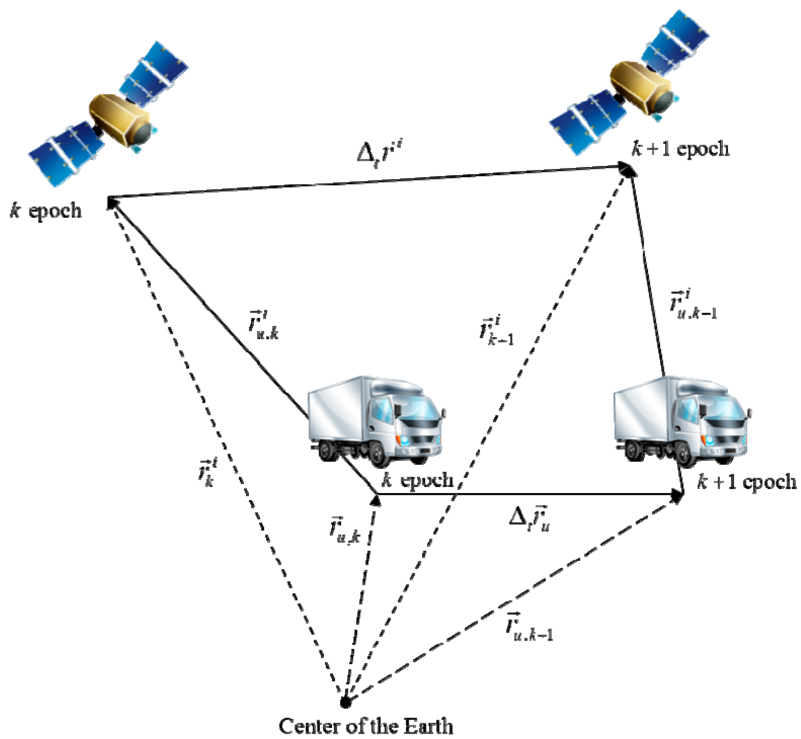
2.1. Monitoring Value for Cycle Slip Detection
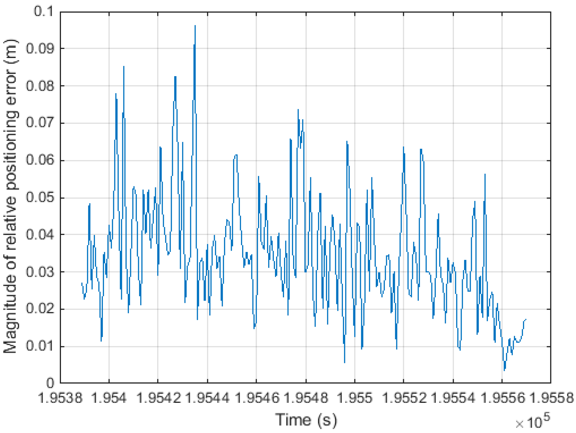
2.1.1. Monitoring Value Error Analysis

2.2. Applying Satellite Geometry to Cycle Slip Detection
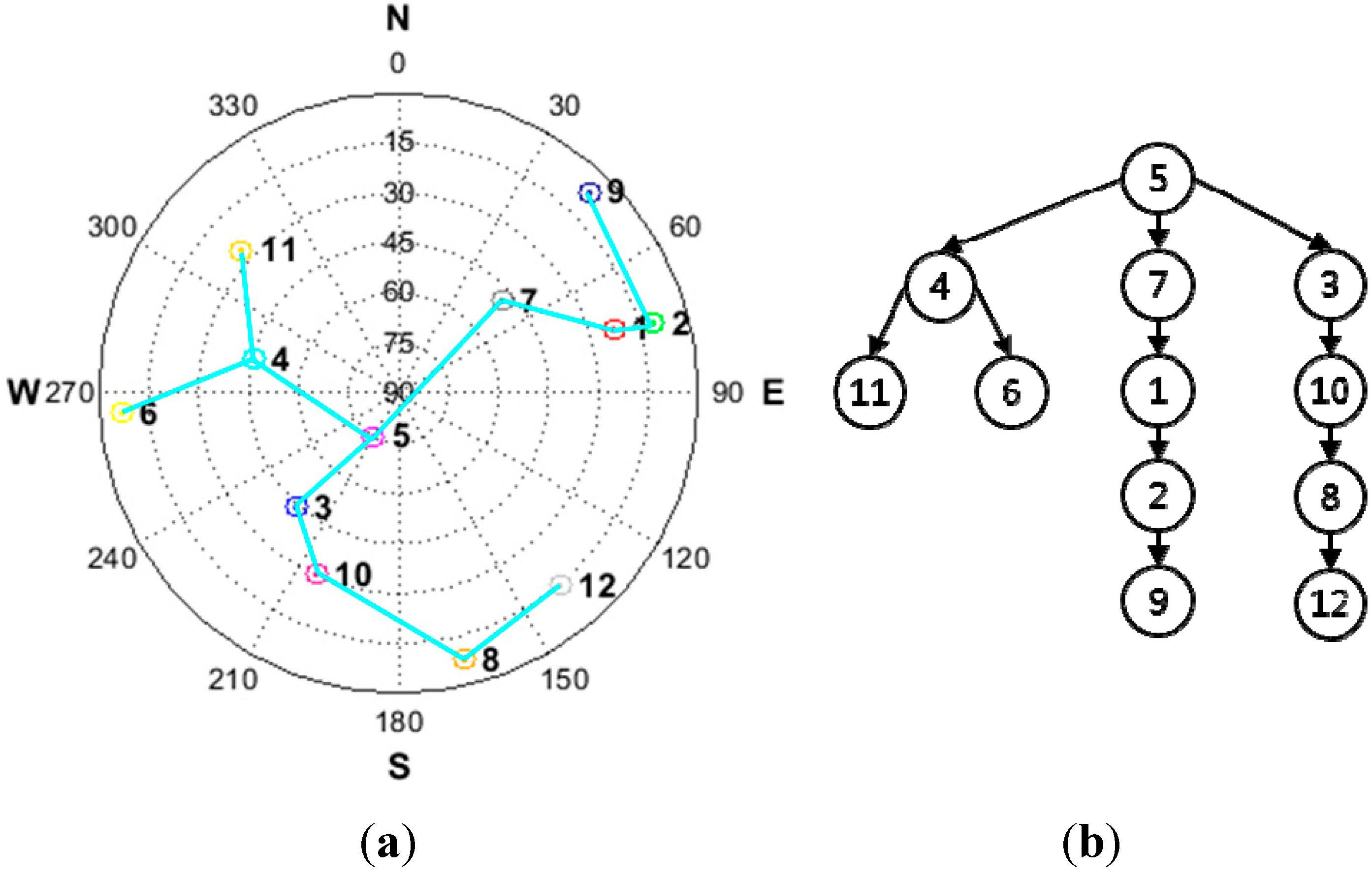
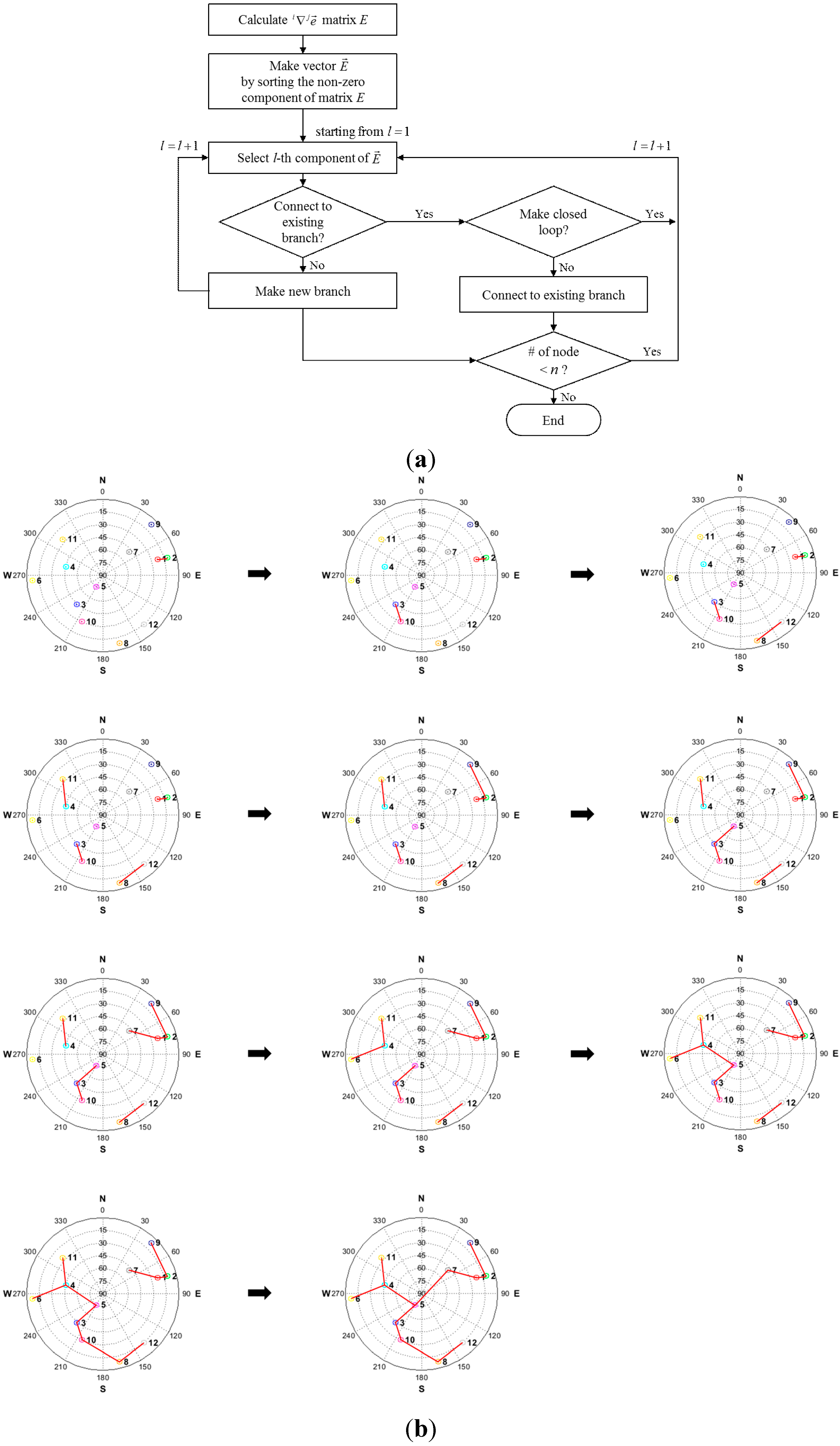
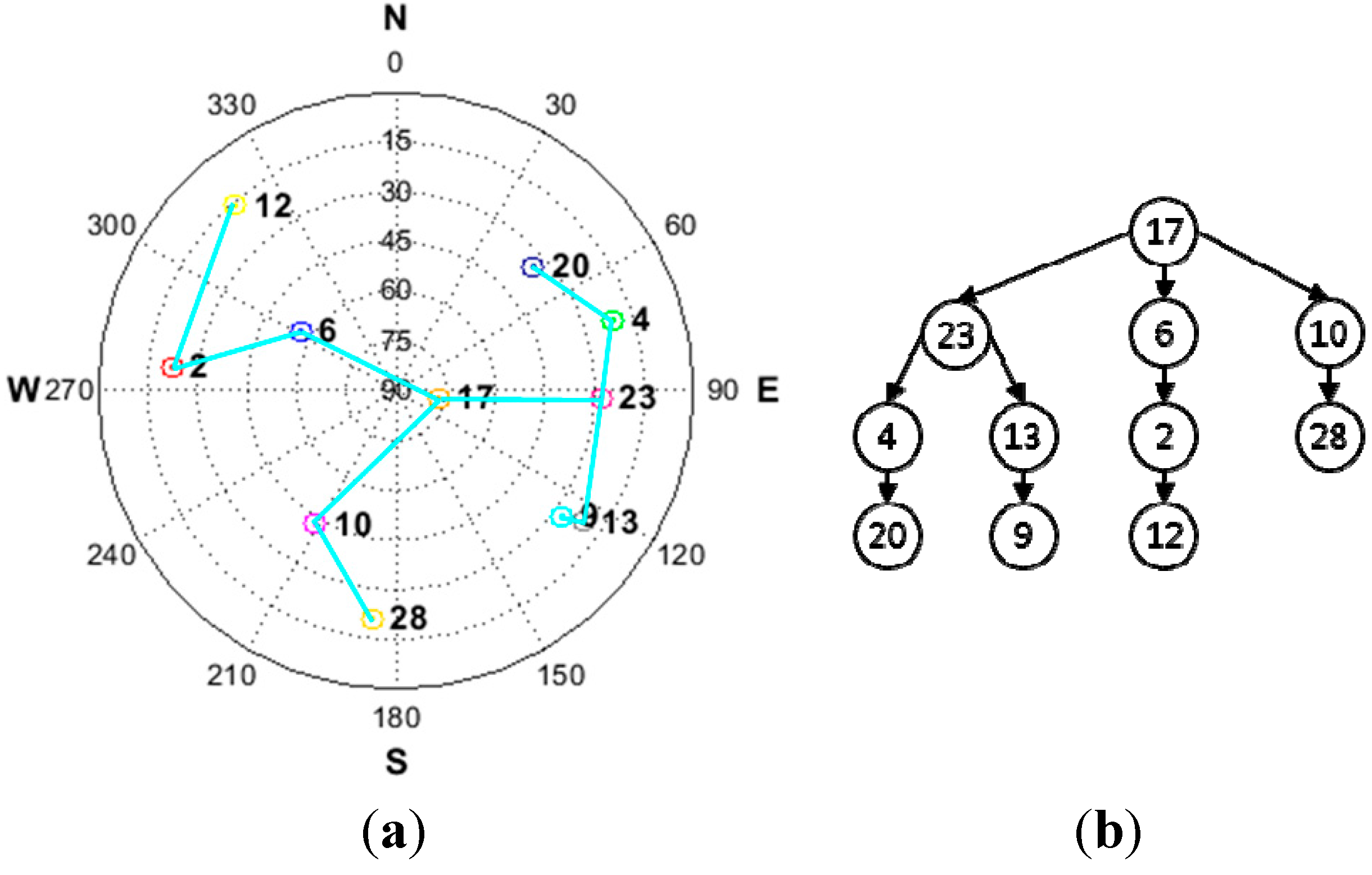
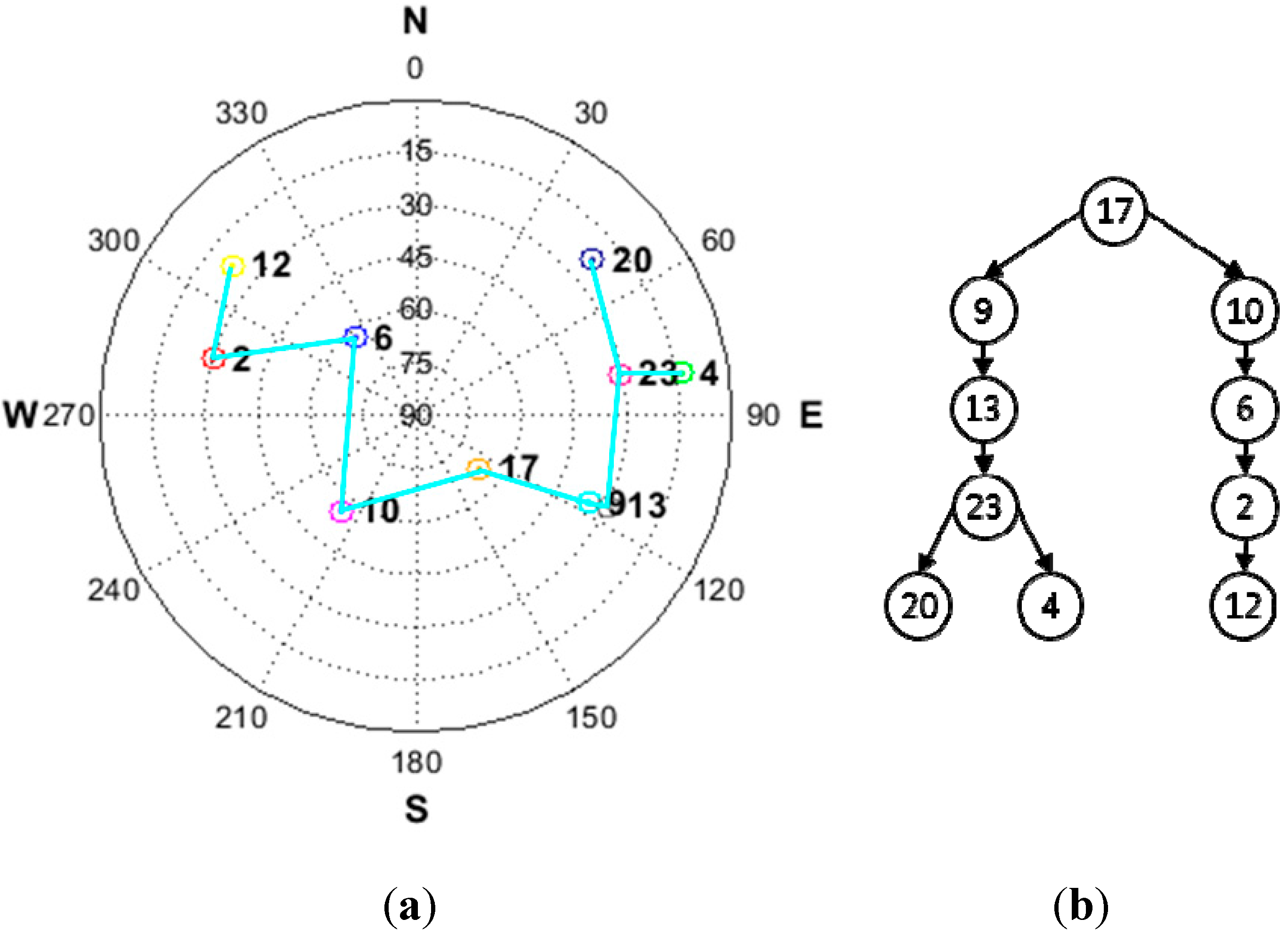
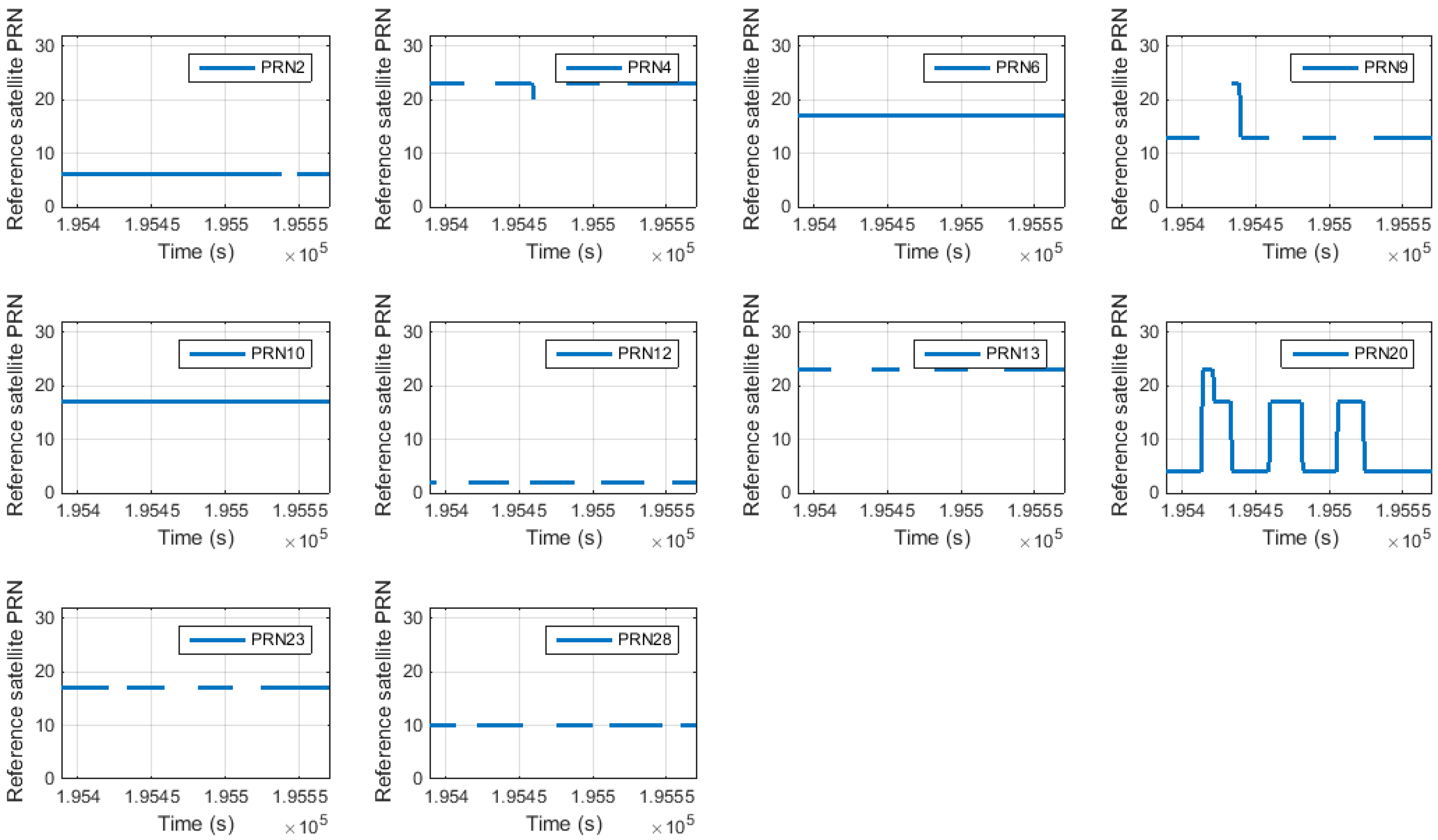
2.2.1. Satellite Pairing

2.2.2. Transformation Matrix for Reconstruction

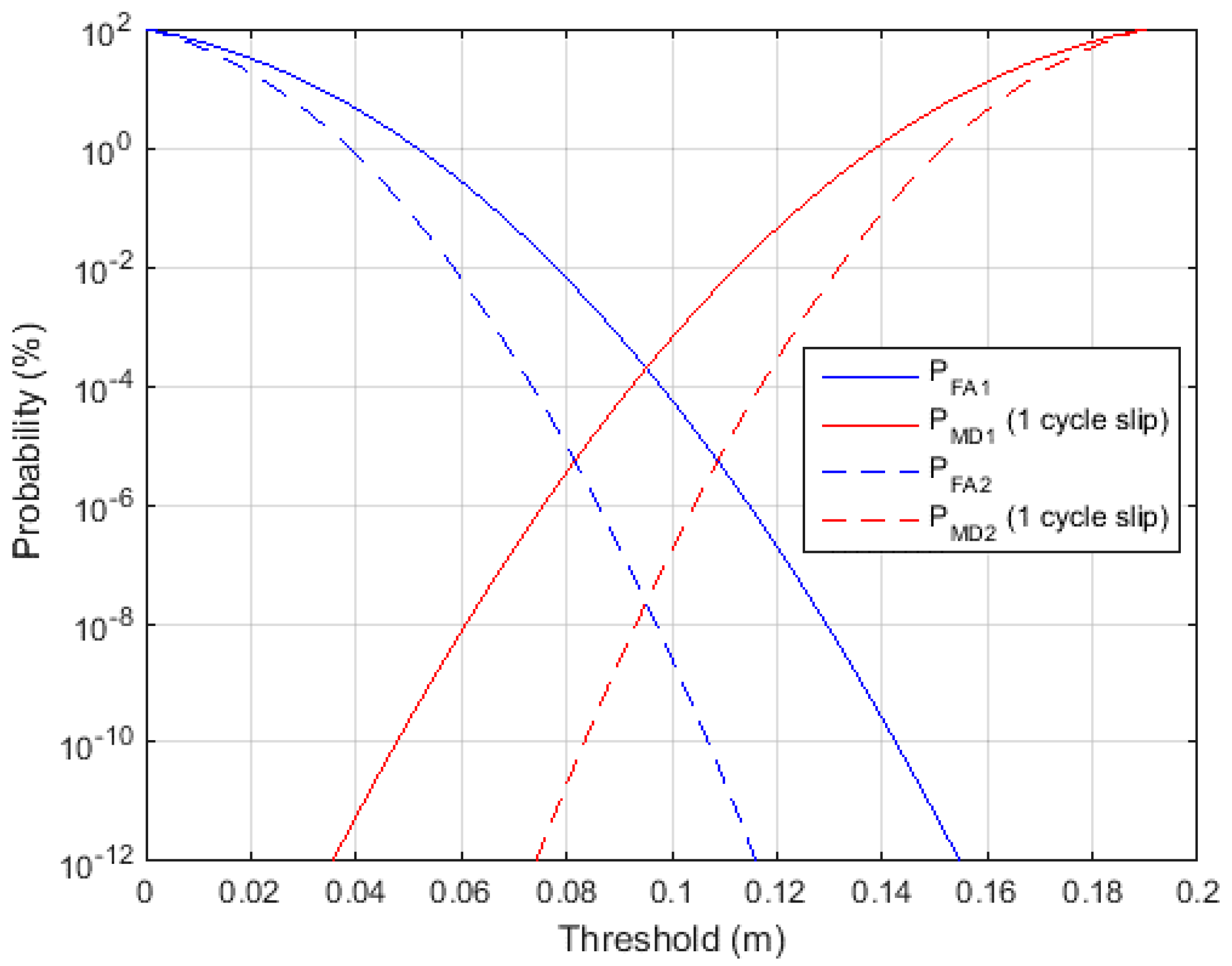
2.3. Cycle Slip Detection Performance Index and Threshold


3. Tightly Coupled TDCP/INS Integration Algorithm

4. Simulation and Experimental Results
4.1. Simulation Results
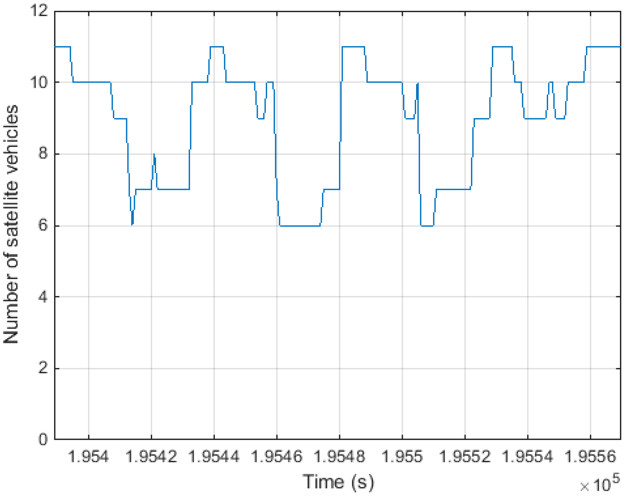
4.1.1. Simulation Environments

| GPS Errors | Generation Strategy |
|---|---|
| Ephemeris error | Neglect |
| Ionospheric delay | Klobuchar model [27] |
| Tropospheric delay | Simplified model [28] |
| Receiver noise | Zero-mean Gaussian noise (σ = 3mm) |
| GPS Errors | Generation Strategy |
|---|---|
| Accelerometer bias | Constant bias (0.1635 m/s2) |
| Gyro bias | Constant bias (1 °/s) |
| Accelerometer noise | Zero-mean Gaussian noise (σ = 0.0333 m/s2) |
| Gyro noise | Zero-mean Gaussian noise (σ = 0.0333 °/s) |
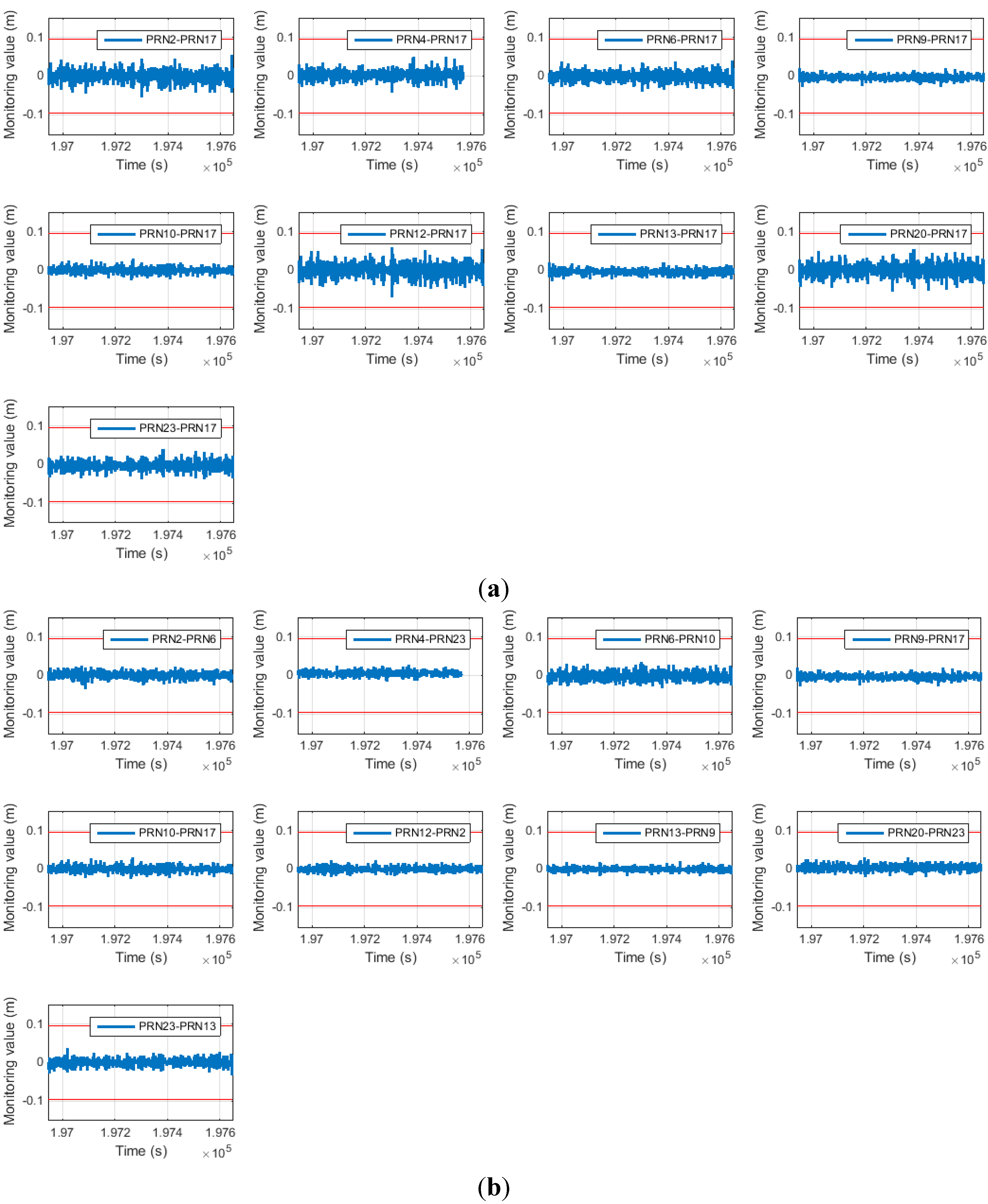
4.1.2. Comparing Monitoring Value Error Performance
| Satellite PRN | σM (General SD) Unit: m | σM (Proposed SD) Unit: m | Error Reduction Unit: % |
|---|---|---|---|
| 2 | 0.0159 | 0.0093 | 41.13 |
| 4 | 0.0131 | 0.0070 | 46.63 |
| 6 | 0.0130 | 0.0121 | 7.03 |
| 9 | 0.0074 | 0.0074 | 0 |
| 10 | 0.0082 | 0.0082 | 0 |
| 12 | 0.0181 | 0.0071 | 60.76 |
| 13 | 0.0081 | 0.0060 | 26.17 |
| 20 | 0.0174 | 0.0083 | 52.15 |
| 23 | 0.0123 | 0.0095 | 23.02 |
| Satellite PRN | PFA (General SD) | PFA (Proposed SD) |
|---|---|---|
| 2 | 2.9127 × 10⁻⁵ | 3.700 × 10⁻¹⁹ |
| 4 | 1.5366 × 10⁻¹² | 0 |
| 6 | 3.1072 × 10⁻⁶ | 3.0773 × 10⁻⁶ |
| 9 | 0 | 0 |
| 10 | 1.8400 × 10⁻¹⁸ | 1.8400 × 10⁻¹⁸ |
| 12 | 3.7533 × 10⁻⁴ | 0 |
| 13 | 0 | 0 |
| 20 | 8.1364 × 10⁻⁵ | 0 |
| 23 | 6.6705 × 10⁻¹¹ | 9.0578 × 10⁻¹² |
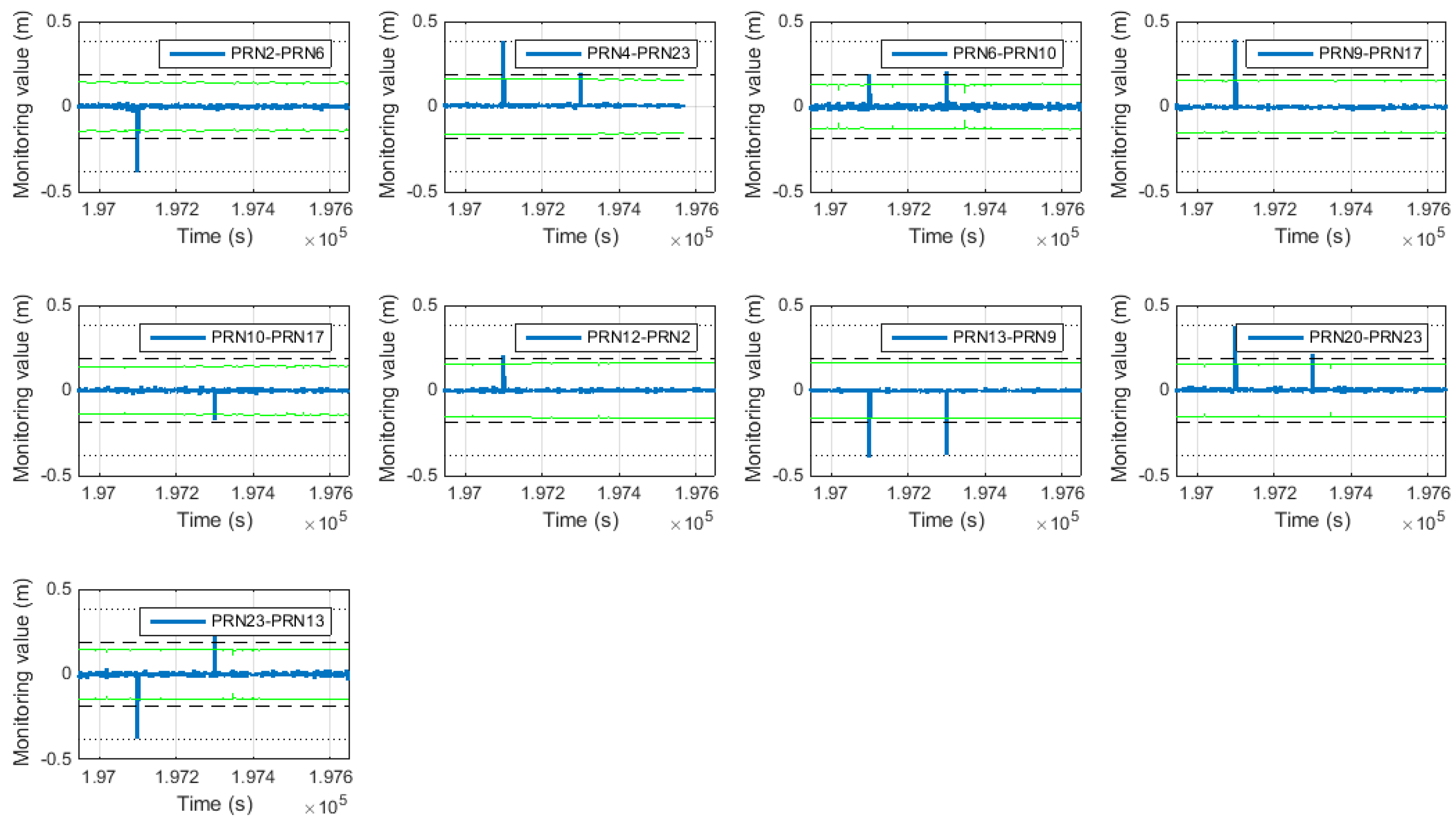
4.1.3. Cycle Slip Occurrence Simulation
| Time Unit: s | PRN | |||||||||
|---|---|---|---|---|---|---|---|---|---|---|
| 2 | 4 | 6 | 9 | 10 | 12 | 13 | 17 | 20 | 23 | |
| 197,100 | −1 | 1 | 2 | −2 | ||||||
| 197,300 | 1 | −1 | −2 | 1 | ||||||
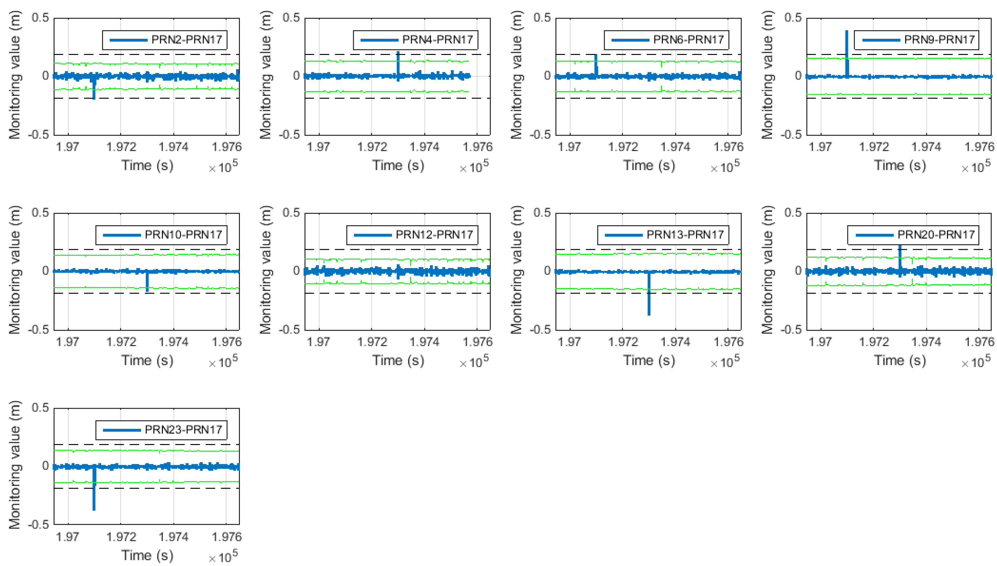
| Time Unit: s | PRN | ||||||||
|---|---|---|---|---|---|---|---|---|---|
| 2–17 | 4–17 | 6–17 | 9–17 | 10–17 | 12–17 | 13–17 | 20–17 | 23–17 | |
| 197,100 | −1 | 1 | 2 | −2 | |||||
| 197,300 | 1 | −1 | −2 | 1 | |||||
| Time Unit: s | PRN | |||||||||
|---|---|---|---|---|---|---|---|---|---|---|
| 2–6 | 4–23 | 6–10 | 9–17 | 10–17 | 12–2 | 13–9 | 20–23 | 23–13 | ||
| 197,100 | −2 | 2 | 1 | 2 | 1 | −2 | 2 | −2 | ||
| 197,300 | 1 | 1 | −1 | −2 | 1 | 2 | ||||
4.2. Experimental Results
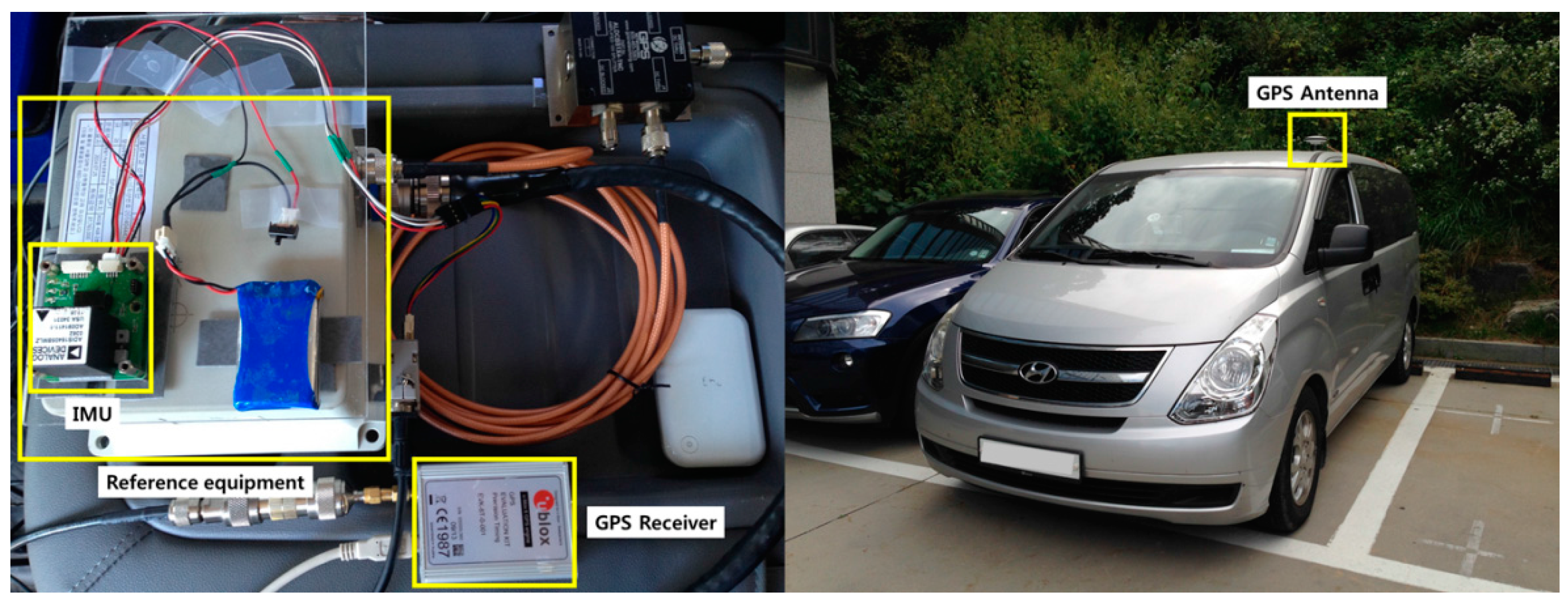
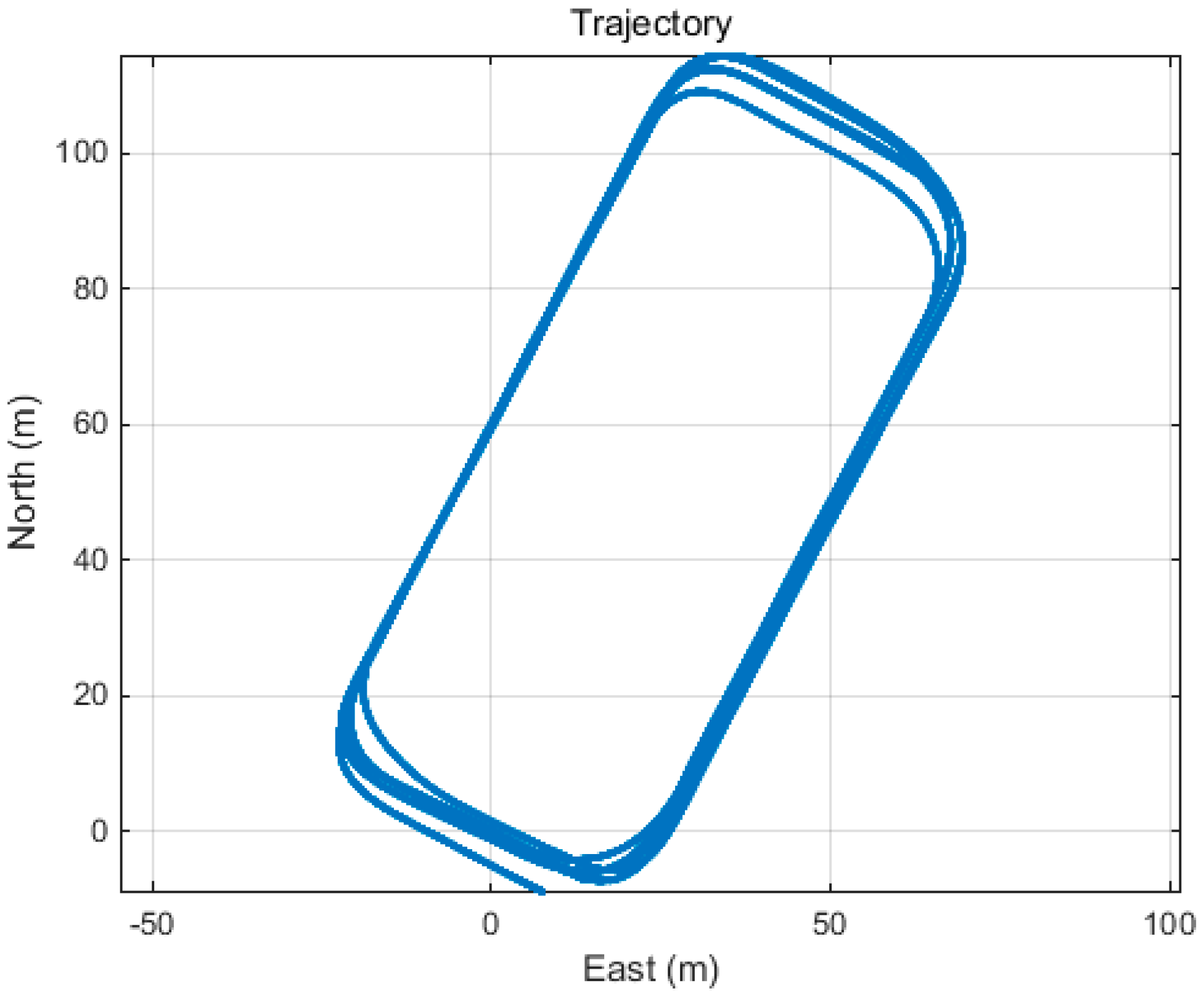
4.2.1. Experimental Environments

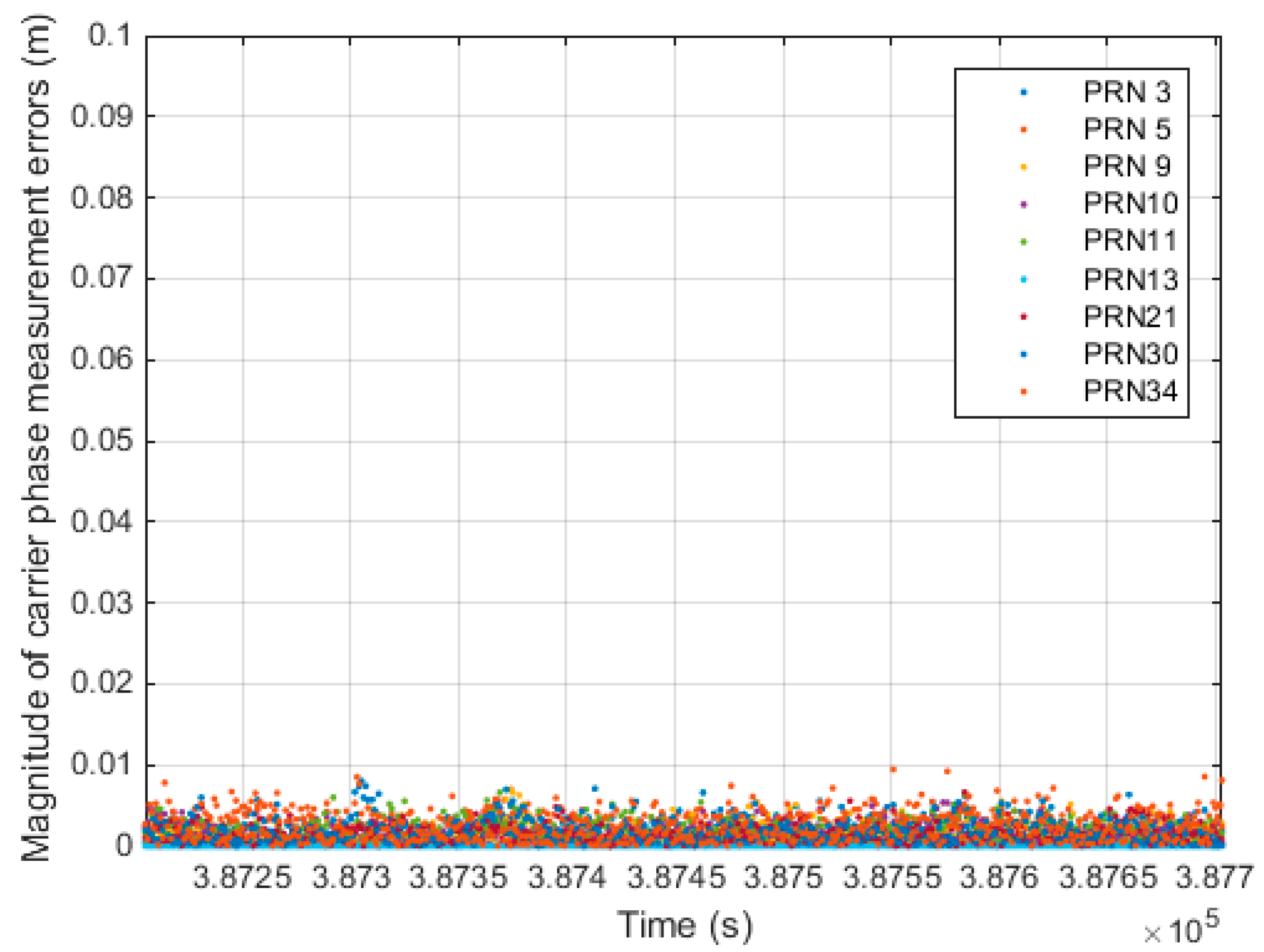
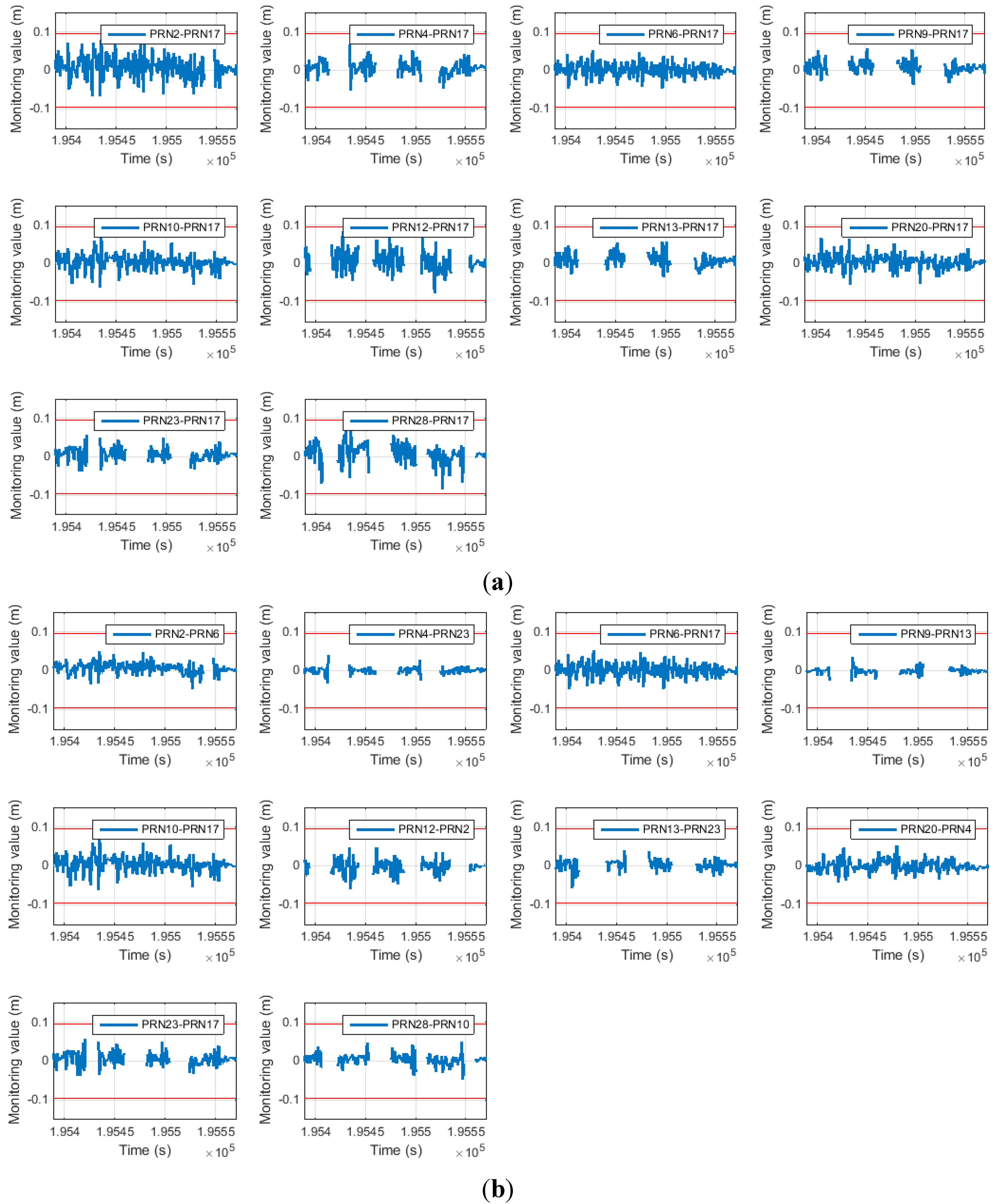
4.2.2. Analysis of Error Sources of Monitoring Value
4.2.3. Comparing Monitoring Value Error Performance
| Satellite PRN | σM (General SD) Unit: m | σM (Proposed SD) Unit: m | Error Reduction Unit: % |
|---|---|---|---|
| 2 | 0.0303 | 0.0153 | 49.67 |
| 4 | 0.0194 | 0.0094 | 51.71 |
| 6 | 0.0187 | 0.0187 | 0 |
| 9 | 0.0173 | 0.0088 | 49.29 |
| 10 | 0.0210 | 0.0210 | 0 |
| 12 | 0.0293 | 0.0191 | 34.87 |
| 13 | 0.0183 | 0.0148 | 19.01 |
| 20 | 0.0193 | 0.0158 | 18.25 |
| 23 | 0.0179 | 0.0179 | 0 |
| 28 | 0.0278 | 0.0155 | 44.37 |
| Satellite PRN | PFA (General SD) | PFA (Proposed SD) |
|---|---|---|
| 2 | 2.1643 × 10⁻² | 2.4368 × 10⁻¹⁴ |
| 4 | 4.5633 × 10⁻⁶ | 0 |
| 6 | 5.4371 × 10⁻⁷ | 5.4371 × 10⁻⁷ |
| 9 | 6.3644 × 10⁻⁸ | 2.4400 × 10⁻¹⁸ |
| 10 | 7.2717 × 10⁻⁶ | 7.2717 × 10⁻⁶ |
| 12 | 2.0212 × 10⁻² | 2.8827 × 10⁻¹⁰ |
| 13 | 2.8758 × 10⁻⁷ | 4.8800 × 10⁻¹⁸ |
| 20 | 1.3231 × 10⁻⁶ | 3.2823 × 10⁻⁷ |
| 23 | 6.5343 × 10⁻⁹ | 6.5343 × 10⁻⁹ |
| 28 | 1.1157 × 10⁻³ | 2.4400 × 10⁻¹⁸ |
4.2.4. Cycle Slip Occurrence Simulation
| Time Unit: s | PRN | ||||||||||
|---|---|---|---|---|---|---|---|---|---|---|---|
| 2 | 4 | 6 | 9 | 10 | 12 | 13 | 17 | 20 | 23 | 28 | |
| 195,441 | 1 | −1 | −1 | −2 | |||||||
| 195,475 | 1 | −3 | −1 | 1 | |||||||
| Time Unit: s | PRN | |||||||||
|---|---|---|---|---|---|---|---|---|---|---|
| 2–17 | 4–17 | 6–17 | 9–17 | 10–17 | 12–17 | 13–17 | 20–17 | 23–17 | 28–17 | |
| 195,441 | 1 | −1 | −1 | −2 | ||||||
| 195,475 | 1 | −3 | −1 | 1 | ||||||
| Time Unit: s | PRN | |||||||||
|---|---|---|---|---|---|---|---|---|---|---|
| 2–6 | 4–23 | 6–17 | 9–13 | 10–17 | 12–2 | 13–23 | 20–4 | 23–17 | 28–10 | |
| 195,441 | 1 | −1 | −2 | −1 | ||||||
| 195,475 | −2 | −2 | −1 | 1 | ||||||
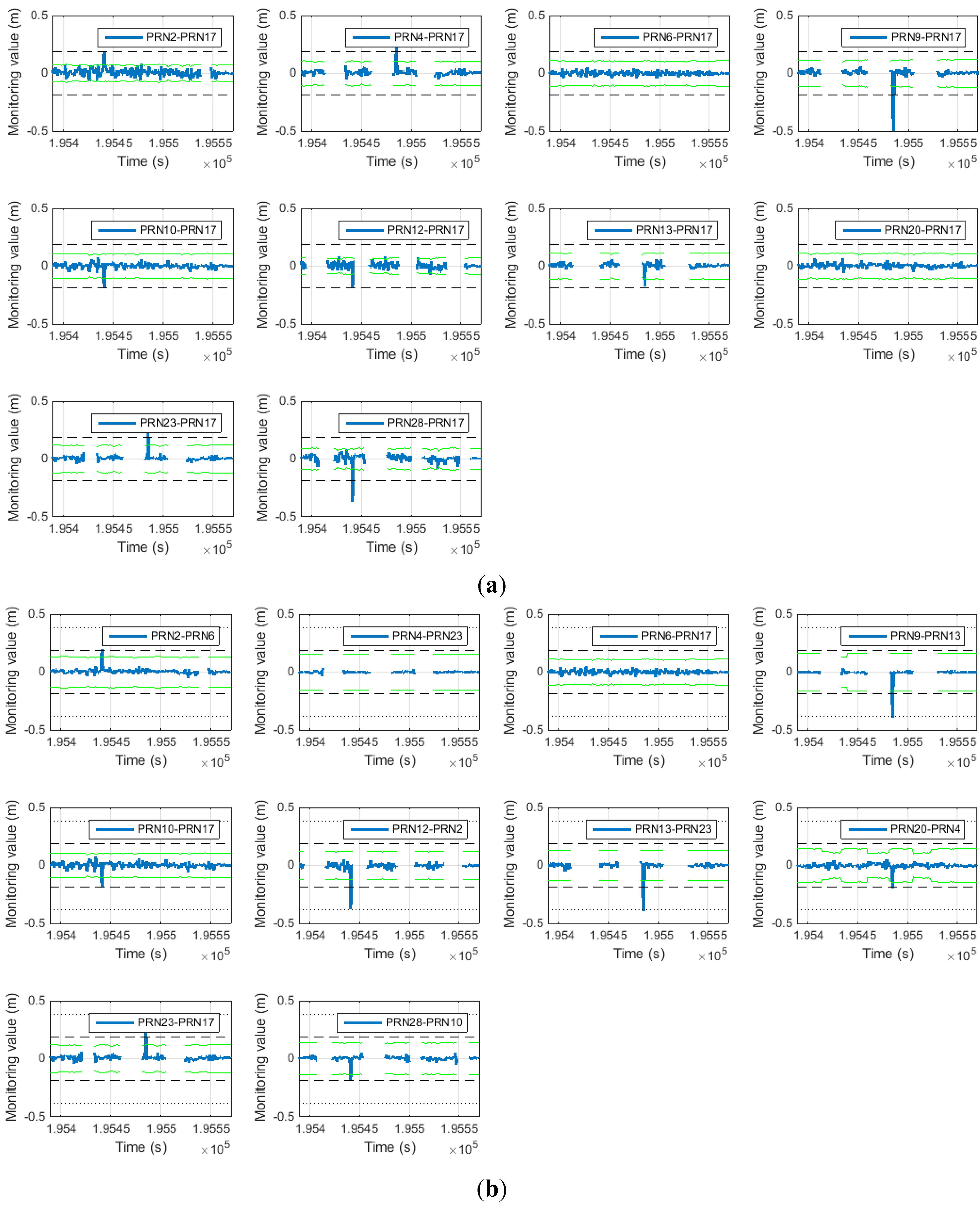
| Method | PRN | |||||||||
|---|---|---|---|---|---|---|---|---|---|---|
| 2 | 4 | 6 | 9 | 10 | 12 | 13 | 20 | 23 | 28 | |
| General SD | 7 | 0 | 0 | 0 | 0 | 5 | 0 | 0 | 0 | 2 |
| Proposed SD | 0 | 0 | 0 | 0 | 0 | 0 | 0 | 0 | 0 | 0 |
4.2.5. Computational Load Analysis
| Computation Time Unit: s | Increase Rate Unit: % | |
|---|---|---|
| General SD | Proposed SD | |
| 30.5 | 32 | 0.05 |
4.3. Summary of Simulation and Experimental Results
5. Conclusions
Acknowledgments
Author Contributions
Conflicts of Interest
References
- Xu, G. GPS: Theory, Algorithms, and Applications, 2nd ed.; Springer: Berlin, Germany; New York, NY, USA, 2007. [Google Scholar]
- Bisnath, S.B. Efficient, automated cycle-slip correction of dual-frequency Kinematic GPS data. In Proceedings of the 13th International Technical Meeting of the Satellite Division of the Institute of Navigation (ION GPS 2000), Salt Lake City, UT, USA, 19–22 September 2000.
- Blewitt, G. An automatic editing algorithm for GPS data. Geophys. Res. Lett. 1990, 17, 199–202. [Google Scholar] [CrossRef]
- Gao, Y.; McLellan, J.F. An analysis of GPS positioning accuracy and reliability with dual-frequency data. In Proceedings of the 9th International Technical Meeting of the Satellite Division of the Institute of Navigation (ION GPS 1996), Kansas City, MO, USA, 17–20 September 1996.
- Gao, L.; Zuofa, L. Cycle slip detection and ambiguity resolution algorithms for dual-frequency GPS data processing. Mar. Geod. 1999, 22, 169–181. [Google Scholar]
- Banville, S.; Langley, R.B. Mitigating the impact of ionospheric cycle slips in GNSS observations. J. Geod. 2013, 87, 179–193. [Google Scholar] [CrossRef]
- Cai, C.; Liu, Z.; Xia, P.; Dai, W. Cycle slip detection and repair for undifferenced GPS observations under high ionospheric activity. GPS Solut. 2013, 17, 247–260. [Google Scholar] [CrossRef]
- Liu, Z. A new automated cycle slip detection and repair method for a single dual-frequency GPS receiver. J. Geod. 2011, 85, 171–183. [Google Scholar] [CrossRef]
- Zhang, X.; Guo, F.; Zhou, P. Improved precise point positioning in the presence of ionospheric scintillation. GPS Solut. 2014, 18, 51–60. [Google Scholar] [CrossRef]
- Ren, Z.; Li, L.; Zhong, J.; Zhao, M.; Shen, Y. A real-time cycle-slip detection and repair method for single frequency GPS receiver. Int. Proc. Comput. Sci. Inf. Technol. 2011, 17, 224–230. [Google Scholar]
- Cederholm, J.P.; Plausinaitis, D. Cycle slip detection in single frequency GPS carrier phase observations using expected doppler shift. Nord. J. Surv. Real Estate Res. 2014, 10, 63–79. [Google Scholar]
- Altmayer, C. Enhancing the integrity of integrated GPS/INS systems by cycle slip detection and correction. In Proceedings of the IEEE Intelligent Vehicles Symposium, Dearborn, MI, USA, 3–5 October 2000; pp. 174–179.
- Colombo, O.L.; Bhapkar, U.V.; Evans, A.G. Inertial-aided cycle-slip detection/correction for precise, long-baseline kinematic GPS. In Proceedings of the 12th International Technical Meeting of the Satellite Division of The Institute of Navigation (ION GPS), Nashville, TN, USA, 14–17 September 1999.
- Takasu, T.; Yasuda, A. Cycle slip detection and fixing by MEMS-IMU/GPS integration for mobile environment RTK-GPS. In Proceedings of the 21st International Technical Meeting of the Satellite Division of the Institute of Navigation (ION GNSS 2008), Savannah, GA, USA, 16–19 September 2008; pp. 64–71.
- Du, S. An inertial aided cycle slip detection and identification method for integrated PPP GPS/MEMS IMU system. In Proceedings of the 24th International Technical Meeting of the Satellite Division of the Institute of Navigation (ION GNSS 2011), Portland, OR, USA, 20–23 September 2001.
- Du, S.; Gao, Y. Inertial aided cycle slip detection and identification for integrated PPP GPS and INS. Sensors 2012, 12, 14344–14362. [Google Scholar] [CrossRef] [PubMed]
- A Matlab Class to Represent the Tree Data Structure. Available online: http://tinevez.github.io/matlab-tree/ (accessed on 8 July 2014).
- Park, B. A Study on Reducing Temporal and Spatial Decorrelation Effect in Gnss Augmentation System: Consideration of the Correction Message Standardization. Ph.D. Thesis, Seoul National University, Department of Mechanical and Aerospace Engineering, Seoul, Korea, 2007. [Google Scholar]
- Song, J.; Kim, Y.; Yun, H.; Park, B.; Kee, C. Predictions of allowable sensor error limit for cycle-slip detection. Trans. Jpn. Soc. Aeronaut. Space Sci. 2014, 57, 169–178. [Google Scholar] [CrossRef]
- Soon, B.K.; Scheding, S.; Lee, H.K.; Durrant-Whyte, H. An approach to aid INS using time-differenced GPS carrier phase (TDCP) measurements. GPS Solut. 2008, 12, 261–271. [Google Scholar] [CrossRef]
- Farrell, J.A.; Barth, M. The Global Positioning Systems & Inertial Navigation; McGraw-Hill: New York, NY, USA, 1999. [Google Scholar]
- Titterton, D.; Weston, J.L. Strapdown Inertial Navigation Technology; IET: Stevenage, UK, 2004. [Google Scholar]
- Rhee, I.; Abdel-Hafez, M.F.; Speyer, J.L. Observability of an integrated GPS/INS during maneuvers. IEEE Trans Aerosp. Electron. Syst. 2004, 40, 526–535. [Google Scholar] [CrossRef]
- Brown, R.G.; Hwang, P.Y. Introduction to random signals and applied Kalman filtering: With matlab exercises and solutions. In Introduction to Random Signals and Applied Kalman Filtering: With MATLAB Exercises and Solutions; Wiley: New York, NY, USA, 1997. [Google Scholar]
- Wendel, J.; Meister, O.; Monikes, R.; Trommer, G. Time-differenced carrier phase measurements for tightly coupled GPS/INS integration. In Proceedings of IEEE/ION PLANS 2006, San Diego, CA, USA, 25–27 April 2006; pp. 54–60.
- Analog Devices. Available online: http://www.analog.com/en/index.html (accessed on 19 November 2013).
- Interface Control Documents of GPS. Available online: http://www.gps.gov/technical/icwg/ICD-GPS-200C.pdf (accessed on 15 December 2014).
- Parkinson, B.W.; Spilker, J.J. Progress in Astronautics and Aeronautics: Global Positioning System: Theory and Applications; AIAA: Reston, VA, USA, 1996. [Google Scholar]
© 2015 by the authors; licensee MDPI, Basel, Switzerland. This article is an open access article distributed under the terms and conditions of the Creative Commons Attribution license (http://creativecommons.org/licenses/by/4.0/).
Share and Cite
Kim, Y.; Song, J.; Kee, C.; Park, B. GPS Cycle Slip Detection Considering Satellite Geometry Based on TDCP/INS Integrated Navigation. Sensors 2015, 15, 25336-25365. https://doi.org/10.3390/s151025336
Kim Y, Song J, Kee C, Park B. GPS Cycle Slip Detection Considering Satellite Geometry Based on TDCP/INS Integrated Navigation. Sensors. 2015; 15(10):25336-25365. https://doi.org/10.3390/s151025336
Chicago/Turabian StyleKim, Younsil, Junesol Song, Changdon Kee, and Byungwoon Park. 2015. "GPS Cycle Slip Detection Considering Satellite Geometry Based on TDCP/INS Integrated Navigation" Sensors 15, no. 10: 25336-25365. https://doi.org/10.3390/s151025336
APA StyleKim, Y., Song, J., Kee, C., & Park, B. (2015). GPS Cycle Slip Detection Considering Satellite Geometry Based on TDCP/INS Integrated Navigation. Sensors, 15(10), 25336-25365. https://doi.org/10.3390/s151025336