Enhancing Indoor Inertial Pedestrian Navigation Using a Shoe-Worn Marker

Abstract
: We propose a novel hybrid inertial sensors-based indoor pedestrian dead reckoning system, aided by computer vision-derived position measurements. In contrast to prior vision-based or vision-aided solutions, where environmental markers were used—either deployed in known positions or extracted directly from it—we use a shoe-fixed marker, which serves as positional reference to an opposite shoe-mounted camera during foot swing, making our system self-contained. Position measurements can be therefore more reliably fed to a complementary unscented Kalman filter, enhancing the accuracy of the estimated travelled path for 78%, compared to using solely zero velocities as pseudo-measurements.1. Introduction
Indoor pedestrian positioning, a prominent example of where Global Navigation Satellite System (GNSS) solutions come up short in terms of performance [1], is a fast growing segment with great potential. This kind of positioning could prove itself to be as useful for the general public (e.g., context-aware applications in airports, shopping malls, libraries, museums, subways, etc.) as for professional users (e.g., helping firefighters and first responders to navigate in low visibility conditions).
Various indoor pedestrian positioning methods have been proposed through the years. Most of the approaches rely either on a modified environment (e.g., radio beacons or fixed visual markers), or some a priori knowledge about it (e.g., radio fingerprinting). In emergency, life-critical scenarios, where time and reliability are of utmost importance, such solutions could be easily stretched beyond their limits. Beauregard [2] has listed a number of demanding, for many technologies prohibitive technical requirements in these worst case scenarios, and also pointed out the time-consuming deployment and calibration of UWB beacon-based positioning systems. Poor visibility and unfavorable lighting conditions can also render unreliable other substantially different approaches, such as a fiducials-free computer vision-based SLAM positioning system—possibly resulting even in completely false position estimation [3]. Rantakokko et al. [4] observed that a robust and accurate first responder positioning system for urban operations requires the use of a multi-sensor approach.
2. Related Work
With the help of modern self-contained inertial sensors the aforementioned shortcomings could be overcome to a certain degree at least. However, the hard to ignore issue of low cost Inertial Measurement Unit (IMU)-based personal navigation systems lays in the inaccuracy of their microelectromechanical system (MEMS)-type sensors. Even with theoretically perfect initial alignment, accurate position tracking can only be successfully performed for a few seconds using commercial grade inertial sensing alone [5], due to cubic-in-time positional error growth caused by angle rates and accelerations integration inherent to the Strapdown Inertial Navigation System (SDINS) algorithm.
To limit the error growth characteristics of low-cost IMU-based pedestrian Inertial Navigation System (INS), also known as Pedestrian Dead Reckoning (PDR), an inherent property of the human gait has been widely exploited—the fact that cyclically one foot at a time stays still on the ground for a short period of time (stance phase) while the opposite one is moving (swing phase) [6]. By taking advantage of this property positional error growth can be decoupled from time, making it linearly proportional to the number of steps taken. Many approaches have been tried in this direction to date, differing by algorithms used, sensors choice and their placement. Foxlin's [7] NavShoe concept represents a substantial upgrade to foot-mounted IMU-based PDRs by introducing the addition of zero velocity updates (ZUPT) as pseudo-measurements to an extended Kalman filter (EKF) during stance phase. Introducing ZUPTs as measurements into the EKF, instead of simply resetting velocity in the SDINS algorithm to zero, brings the substantial advantage of a retroactive correction of the state vector. More recently, the ZUPT approach was used by Alvarez et al. [8] in a waist-worn inertial personal navigation system that can be precise enough for some applications.
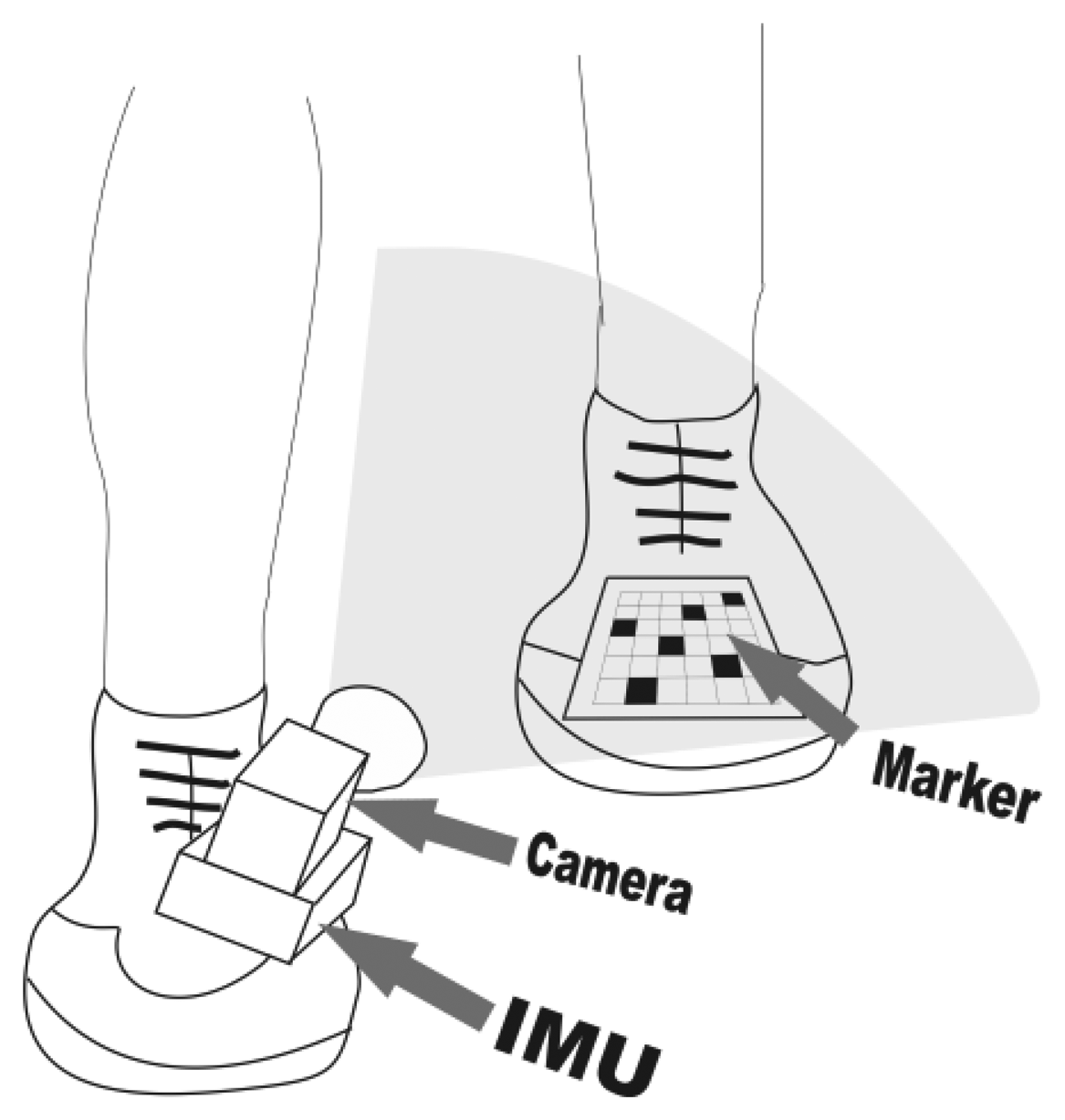
Considerable research has been carried out recently in the hybrid indoor positioning field. Having in mind that most of the presented hybrid approaches are not self-contained or rely on environmental features [9] and that a lot of research has been done in heading estimation improvement for PDR, we sought to engage an innovative way to somehow enhance the original ZUPT approach, especially in difficult, typical first-responder scenarios. The result is our low-cost, proof-of-concept hybrid PDR depicted in Figure 1. Computer vision was chosen as the aiding modality because of its complementarity to inertial sensing as Corke et al. pointed out in [10], while the desire to simultaneously decrease the dependence of the system on environmental features led us to think in the direction of a wearable marker. To the best of our knowledge, no general pedestrian navigation platform, that would allow a seamless blending of visual sensory information, is available at the moment. The modular multi-sensor pedestrian location and navigation platform with integrated data timestamping that Morrison et al. describe in [11] seems very close to this aim, but it does not support video input in its present iteration.
Our approach is similar to the one proposed by Do and Suh with their Gait Analysis System [12] for the fact that it uses a shoe-mounted IMU with a rigidly connected camera. The crucial difference comes in the placement of the visual marker. We opted for a shoe-fixed marker on the opposite foot, serving as a positional reference to the IMU-camera-compass (IMUCC) unit, mounted onto the other shoe. Using a self-attached visual marker as a positional reference for a combined IMUCC unit is a novel approach, since visual markers are usually pre-deployed into the environment.
We therefore propose a novel, self-contained machine vision-aided hybrid PDR aiming to improve foot trajectory estimation in an IMU-based PDR system with ZUPTs. The idea is to minimize foot trajectory error during the swing phase, particularly during slow or disturbed walking, when the swing phase, and thus the error integration time, may last longer. We achieve our goal by taking advantage of a novel visual marker-based setup, where traditional environmental markers are being replaced by a user-worn marker, fixed on the user's shoe, while an IMUCC unit is placed on the opposite one. From the time it enters in the camera's field of view, the marker's pose with respect to the camera can be determined by means of an augmented reality (AR) machine vision algorithm and from then on it can serve as a positional reference to the IMU, since there is a fixed, known spatial relationship between the camera coordinate frame and the IMU coordinate frame. Position measurements can be therefore fed to a complementary unscented Kalman filter (UKF), operating in a unit quaternion space in feedback configuration.
3. System Description
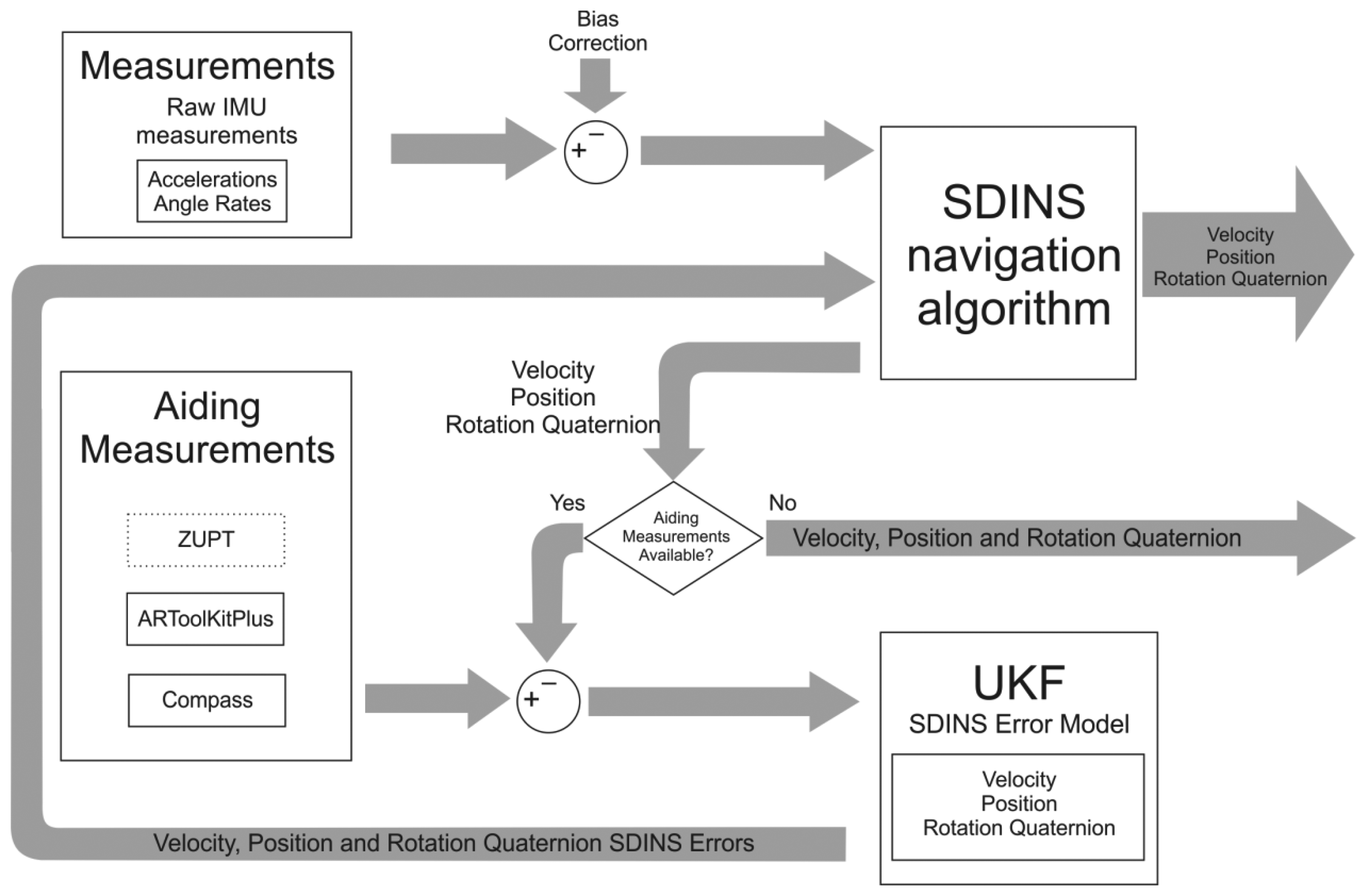
In this section a description of the proposed algorithm will be given. Its schematic representation is shown in Figure 2. Emphasis will be put on aiding measurements and filtering algorithms, whereas the SDINS navigation algorithm in quaternion approach will be treated in the Appendix section at the end of this article.
3.1. Coordinate Systems and Notation
We make use of the following Cartesian, orthogonal coordinate reference systems (frames) throughout the article:
Inertial (i-frame) is the inertial frame, fixed with respect to the stars with the origin in the center of the Earth. All inertial measurements are done with respect to this frame.
Earth (e-frame) is the Earth centered and fixed frame. This frame is of limited use in our case, but of great importance using higher accuracy IMUs in long distance and high dynamics outdoor missions.
Local NED (n-frame) is the local level frame at the SDINS computed position, following the NED (north-east-down) notation.
Navigation (nav-frame) is the local level frame at the first SDINS computed position. In our case, using a low-cost IMU, not capable of Earth-rate sensing, in low dynamics conditions for short periods of time, we neglect Earth's curvature and rotation, making possible to assume the alignment of the nav-frame and n-frame. We use the NED notation for this frame. Camera pose is being calculated with respect to this frame.
IMU (b-frame) is the coordinate frame of the body—in our case the frame of the IMU, which is attached to the shoe. All the inertial measurements are being measured in this frame.
Camera (cam-frame) is the coordinate system of the camera, which is rigidly connected to the IMU unit. The z axis is pointing along the optical axis, starting from the optical center of the camera, its x axis perpendicular to the z axis to the right.
Reference Marker (mref-frame) is the coordinate system of the first recognized marker during the swing phase, which serves as a reference to the subsequent ARToolKitPlus measurements that occur later during the current swing phase.
Marker (m-frame) is the marker coordinate frame. It is fixed onto the user's opposite shoe with the z axis pointing out from the marker and the x axis pointing perpendicular to the z axis to the left.
Platform (p-frame) is the SDINS software frame in which the transformed inertial quantities (accelerations and angular rates) are being solved. In the ideal case the p-frame and n-frame would be parallel, but because of the errors, inherent to inertial sensors, a discrepancy arise. The p-frame axes configuration copies that of the n-frame.
All frames are right-handed, the third axes are thus defined with the first two. In this article superscript is used to denote the coordinate system in which a variable is represented. Bold text is used for vector and matrix variables.
3.2. Visual Position Estimation Using a Shoe-Mounted Marker
The main idea behind our approach was motivated by the fact that SDINS positional uncertainty grows cubically over time. Developing a method to somehow anchor subsequent foot position measurements during swing phase, when SDINS calculations keep losing accuracy, to a prior point in time, when accuracy was greater, was our goal. The use of a shoe-worn marker would allow us to perform positional measurements with accuracy that is substantially decoupled from time, similarly to using an outdoor operating GNSS receiver. The cubical position error growth of the inertial-only SDINS solution during the swing phase should therefore become limited to the sum of the positional error, which occurred up to the time of the reference marker image acquisition and the inherent ARToolKitPlus [13] positional measurement error. Using visual position estimation, an enhanced navigation solution is expected, when longer SDINS integration times occur (i.e., during slow walk), compared to a SDINS algorithm using only ZUPT pseudo-measurements.
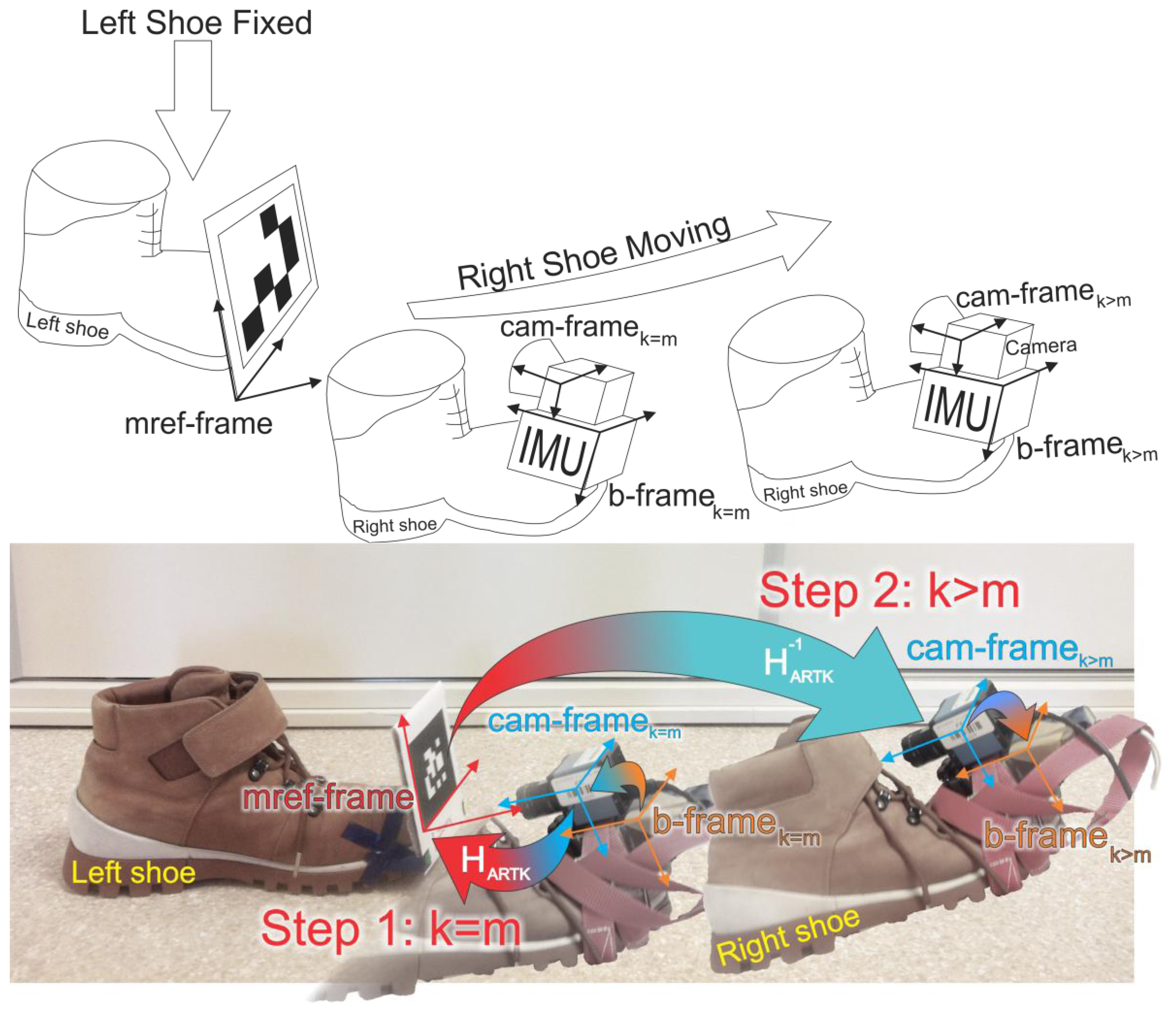
The coordinate systems transformations involved, leading to the actual positional measurement being fed to the UKF, can be thought of as a two-step process (Figure 3):
When the marker is first recognized in an image during the swing phase, its 3D pose is calculated with the aid of the IMU frame calculated pose in the nav-frame, the known IMU-Camera lever arm and the current ARToolKitPlus measurement of the pose of the marker in the cam-frame. We call this resulting frame the reference marker coordinate frame (mref-frame).
From now on the system's computational workflow reverses with respect to the first step. The inverse of the ARToolkitPlus homogeneous matrix is used to perform the transform from the previously calculated mref-frame, expressed in the nav-frame, to the cam-frame and again the known IMU-Camera lever arm transformations are used at the end for calculating the actual homogeneous matrix, describing the pose of the IMU frame in the navigation frame.
The visual marker-based relative 3D positional measurement architecture that we are using relies on the well-known ARToolKitPlus AR framework, which is based on the pose estimation algorithm developed by Schweighofer and Pinz [14]. Before an image can be efficiently used as a measurement, the camera unit has to be calibrated to compensate for optical distortions caused by the lens. With the aid of the Camera Calibration Toolbox for MATLAB [15] and a printed checkerboard pattern we have determined the intrinsic parameters of the camera-lens combination and rectified the images before they were fed to the ARToolKitPlus for image processing.
A common characteristic of optical tracking AR systems with fiducial markers are their viewing angle W-shaped rotation error functions [16,17]. With this in mind we tried to mount the marker in a way that it would remain outside of lower accuracy regions throughout the whole swing phase, because not only position, but the whole pose information (i.e., including orientation) was used later in calculations. When fixing the marker onto the shoe, we therefore rotated the marker for a few degrees towards the camera around its yaw axis and slightly increased its pitch, compared to a marker facing directly into the walking direction.
Our camera is rigidly connected to the IMU. Using the calibration algorithm developed by Hol et al. [18], high quality estimates of the relative orientation between the camera frame and the IMU frame could be determined. However, we chose to follow a more straightforward, yet effective approach: to a first approximation, in our paper we assume that the camera axes are either completely parallel or perpendicular to the IMU axes. Translation offsets between the center of the IMU and the sensor of the camera were accurately measured with the aid of a Vernier caliper. Knowing both rotational and translational relationships between the b-frame and cam-frame, homogeneous matrix transforms needed to convert back and forth between the two coordinate systems can be determined.
3.3. Data Synchronization
Having three separate measurement data streams of mutually dependent quantities, one for visual marker pose measurements, one for inertial measurements and one for magnetic compass heading measurements, gives rise to the data synchronization issue. The most accurate and straightforward solution in our case would be to use a hardware-based time synchronization mechanism for the three streams, similarly to [18]. Not having such a system at hand, we opted for a more Ad-Hoc approach since all computations are made off-line. We logged inertial serial data sentences at 156 Hz, video frames were taken at a fixed rate of 15 Hz and magnetic compass readings at 20 Hz. While recording all data streams (inertial, video and compass) simultaneously we completed a quick rotation of the combined IMUCC unit, making sure the marker does not leave the camera's field of view during the move. We then applied our SDINS algorithm to the recorded inertial data, extracted the computed IMU orientations and transformed them into camera Roll-Pitch-Yaw (RPY) orientations. Since visual marker trackers give the most accurate rotation estimation results for roll rotation (around the z axis of the cam-frame) [17], we had accomplished the time-synchronization procedure with regard to this rotation. For synchronizing the compass data stream we took advantage of the roll readings in the compass output sentences. At this point we had three different data streams representing the same quantity (IMUCC unit roll), one lagging another for an unknown amount of time. We then had to resample the data sets to the same frequency—we chose to resample the less-frequently sampled camera orientation and compass roll data streams to the same frequency as the IMU data to prevent precision reduction of the final synchronization result. We used quadratic instead of linear interpolation to achieve a slightly smoother resampled curve. The final step of the data synchronization procedure was to determine the lag among data streams by comparing the derivatives of the orientation curves extracted from all three modalities.
3.4. Filtering Algorithms
3.4.1. The Error State Vector
Complementary filtering involves system error estimation through system error modeling. Therefore, the states used in our complementary filter architecture are SDINS velocity and position errors in the n-frame and quaternion attitude error between the p-frame and n-frame. All states used in a Kalman filter are considered to be white-noise driven signals. Any time-correlated driving noise should be properly shaped. In most cases, a first-order Gauss-Markov process model is accurate enough for modeling such errors. The state vector is then augmented with additional states to accommodate these additional colored noise states. To use this approach is particularly important in long lasting missions using sensors with non-negligible sensor drift, where the filter is augmented with accelerometer and gyro bias states. However, because the noise power spectral density (PSD) curve of the IMU outputs showed negligible drifts for the duration of our proof-of-concept experiments, we considered accelerometer and gyro biases as zero mean white noises in our article for simplicity and clarity reasons.
Therefore, considering velocity, position and attitude as the main quantities of interest in a navigation solution and sensor biases as time uncorrelated states, we can define the following error state vector for our complementary UKF:
As it can be observed above, the filter error state vector is composed of a translational part (Δvn and Δvnav) and a rotational part ( ). Representing the rotational part of the filter with quaternions means that common vector space UKF cannot be used for propagating the whole state vector in time, because of the unit quaternion departure from the unit sphere due to the addition and multiplication operation in the weighted mean procedure. We therefore chose to combine two separate versions of unscented transform (UT) operating on a common state vector for error state propagation, a translational UT in vector space for velocity and position error propagation, and a rotational UT in unit quaternion space for attitude error states propagation.
3.4.2. Translational UKF in Vector Space
The unscented Kalman filter constitutes an alternative to the extended Kalman filter, which is a suboptimal implementation of the recursive Bayesian estimation framework applied to Gaussian random variables [19]. Developed for nonlinear process and measurement models in estimation and control problems, it is based on the principle that it is easier to approximate a Gaussian distribution than it is to approximate an arbitrary nonlinear function, making cumbersome Jacobian or Hessian calculations, which are the base for derivative-based filters like it is the EKF, superfluous. In the UKF, sample points (also called sigma points) are propagated through a nonlinear system, but, unlike in particle filters, a minimal set of sample points is deterministically chosen to capture the posterior mean and covariance of a random variable up to the 2nd order.
A complementary filter operates on the navigation errors in the error state space, recursively estimating them, making it possible to correct navigation states in the total state space SDINS. We have not employed any small angle assumption in the development of the algorithm. A complementary UKF in a unit quaternion space was developed for the rotational (unit quaternion) part of the state vector propagation, while a vector space complementary UKF was used for the Euclidean vector space part of the state vector. Hereafter in this chapter we will describe the fundamental algorithm of the latter.
Considering the following discrete-time process governed by the nonlinear stochastic difference equation:
3.4.3. Rotational UKF in a Unit Quaternion Space
In contrast to vector quantities, rotations lie on a nonlinear manifold and quaternions, used in our system to represent them, are constrained to a unit radius hypersphere in a four-dimensional Euclidean space (a 3-sphere). This is the reason why quaternions are not closed for addition and scalar multiplication (operations that constitute the core of the weighted sum calculations in an UKF) and consequently why using unscented filtering directly with a unit quaternion attitude parametrization generally yields a non-unit quaternion estimate [21].
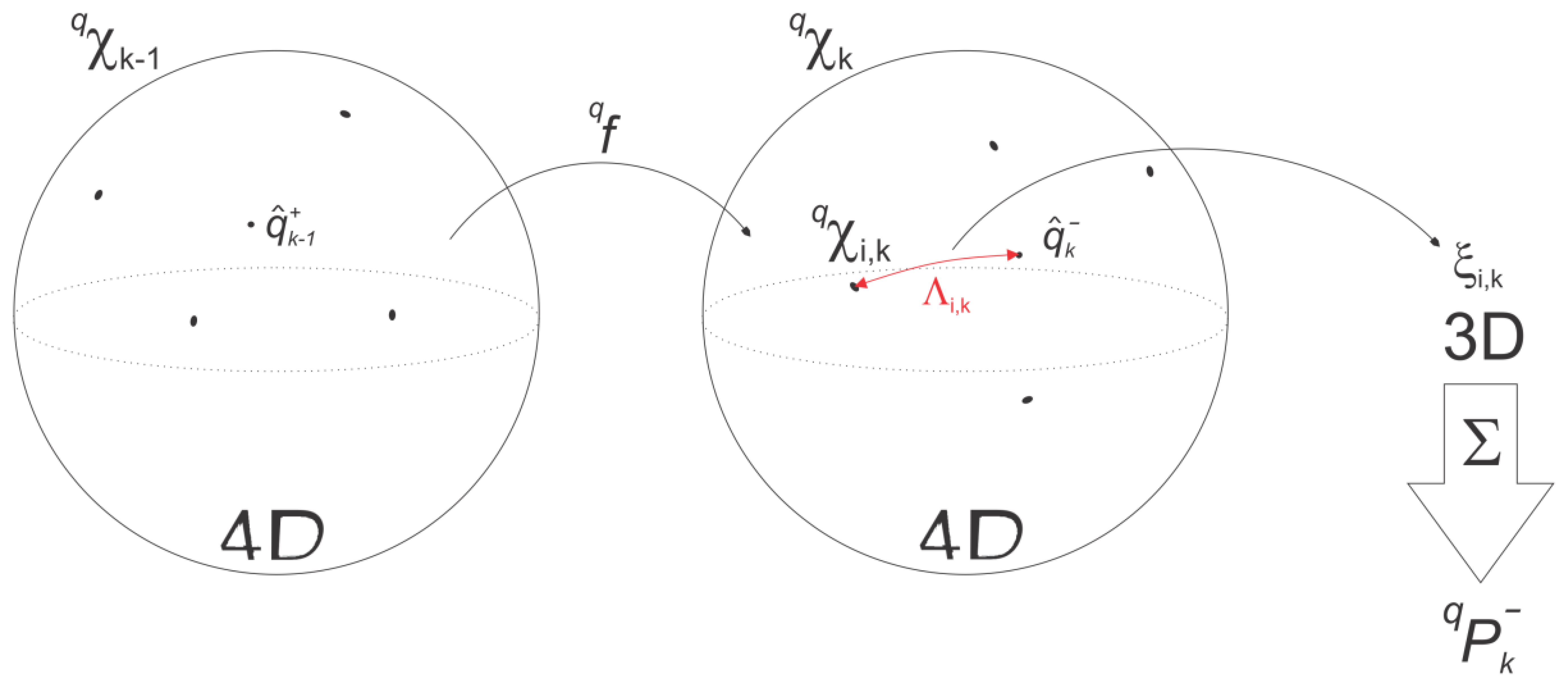
The original vector space UKF algorithm has thus to be modified accordingly to ensure that during the weighted sum of the unscented transform, the quaternion does not depart from the unit sphere. This was achieved with the help of the rotation vector attitude representation for sigma point rotation vector generation, followed by a quaternion-based weighted mean computation based on the quaternion distance metric formulated in [22] (Figure 4). A more in-depth description of the rotational filter algorithm is given below.
We chose to treat the quaternion noise (the equivalent to wk−1 in the vector space UKF, where the superscript + denotes the post-update process noise estimate when gyro bias error is being considered) as a rotation vector, because this way the transformed sigma points are more narrowly scattered around the current estimate compared to the alternative noise representation as a vector part of the quaternion [23]:
Dealing with a combined translation-rotational UKF, we would like to emphasize that (2n + 1) sigma points have to be generated for the combined filter, meaning that using the rotation vector representation for rotational sigma point generation, 19 sigma points have to be generated (n = 9). This set of transformed quaternions is then propagated forward in time through the rotational part of the process model qf yielding the new set qχk:
The predicted mean quaternion part of the error state vector ( ) is then determined as the barycentric mean with renormalization:
The associated predicted rotational covariance is computed by first finding the distance Λi between the single sigma quaternion and the predicted mean quaternion:
Each quaternion distance Λi,k is then converted to the equivalent distance rotation vector ξi,k with the following equation:
Propagating the quaternion sigma points through the measurement model:
3.4.4. Measurement Modes
Since we are using three different measurement modalities, namely ZUPT, visual position measurement (ARTK) and heading measurement (Figure 2), our system has to deal with three distinct measurement modes, each with a different observation matrix H. In the ZUPT pseudo-measurement mode (we make use of the “pseudo” prefix throughout the article because these observations are not actual measurements, but the assumed zero velocities) the observation matrix selects the velocity states, in the ARTK position measurement the H matrix selects the three position states, while in the case of a heading measurement the four orientation quaternion states are selected from the filter error state vector, which are consequently converted to a rotation vector during the UKF sigma points calculations. This back and forth conversion between the nine and ten states is required because of the covariance computation within the rotational part of the filter [24].
The measurement switching module sets the ARTK measurement mode each time the marker is recognized in the image and a position measurement is therefore available, while an effective and straightforward gyro signals thresholding technique similar to Foxlin's approach in [7] is used to enable the ZUPT pseudo-measurement mode. Foxlin's one-heading-measurement-per-step approach was used for heading measurement update—we performed it once per step to limit the effects of the colored environmental magnetic noise, at the time of the first ZUPT pseudo-measurement in the detected stance phase, because at that time the compass measurement should have been stabilized already. In the measurement update stage of the filter ZUPT mode was set to higher priority than the ARTK mode, because of the lower uncertainty of its pseudo-measurements, while the time update-only stage was performed during the swing phase without any external observations, to update the states error covariance in the UKF due to inertial sensor errors.
Dealing with complementary filter architecture, we have to stress the fact that the measurements zk involved in the update stage of the filter are actually difference quantities δzk, i.e., errors between the measurements and the respective estimated total states. Since linear velocities belong to the Euclidean vector space, arithmetic subtraction can be performed to get the actual measurement δvZk fed to the filter when performing in the ZUPT pseudo-measurement mode:
In heading measurement mode we are dealing with rotation measurements represented by unit quaternions, which are not mathematically closed for subtraction. We thus opted for the following quaternion multiplication approach to get the heading error measurement to be fed to the UKF in a complementary configuration. Heading was first extracted from the SDINS attitude quaternion by converting it to the rotation matrix notation, then subtracted from the compass heading measurement and the result converted to a difference rotation quaternion δqzk,which represents the measured difference rotation quaternion to be fed to the UKF:
It has to be noted that heading measurements are presented as attitude measurements to the UKF in the heading measurement mode, therefore the generally nonlinear measurement transfer model h is represented by a linear matrix transform HeadingH, which directly mirrors the measurements to the respective quaternion attitude states. Consequently, distance vectors ξi,k belonging to the quaternion sigma point set qχi,k, belong to the propagated set qγi,k as well. We take advantage of this property in the cross correlation matrix calculations below.
In the ARTK measurement mode the difference δrzk between the IMU's ARTK measured position and the SDINS estimated position of the IMU sensor is being fed to the UKF:
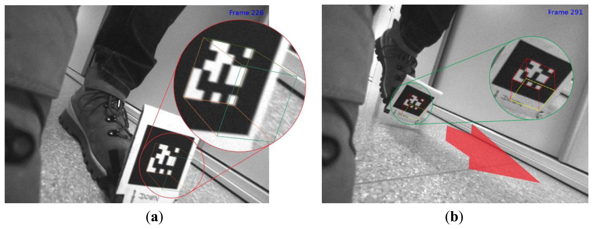
Regarding the ARTK measurement mode, a few words need to be devoted to its triggering. First of all, only pose measurements with high confidence are taken into account in the UKF, since frames (measurements) with lower ARToolkitPlus confidence tended to produce poor 3D cube overlays (Figure 5a), which meant 3D marker pose estimations were inaccurately determined for some reason. Since low confidence ARToolKitPlus measurements occurred rarely, simply discarding those measurements proved to be an effective strategy to cope with this phenomenon. Secondly, ARTK measurement mode has to be triggered only when the marker-equipped foot is stationary on the floor to allow precise 3D pose measurement of the reference marker coordinate frame and also of all successive camera coordinate frames during the swing phase of the IMUCC-equipped foot. However, marker pose measurements are often available during the stance phase, just before heading and subsequent ZUPT measurement mode triggering occur (Figure 5b). To effectively reject these inadequate measurements, velocity thresholding was implemented, i.e., if the calculated velocity of the IMUCC unit fell below a certain value, then the ARTK triggering signal was not passed through to enable the ARTK measurement mode in the UKF. To allow ARTK positional measurements during midair interrupted swings, when the foot would almost hover over the floor, some other kind of triggering strategy has to be employed, e.g., SDINS height triggering or using a shoe with an integrated ground contact sole switch.
3.4.5. Kalman Gain and Measurement Update Equations
The UKF gain Kk is obtained with:
The cross correlation matrix for the rotational part of the filter cannot be calculated using quaternion subtraction. Hence, the rotation vector is used as the distance measure again:
We can define the error state vector and covariance as:
Since we are dealing with a complementary filter architecture, SDINS states have to be updated by the error state vector . We refresh the SDINS states after a measurement update stage occurs, as described below, leaving the error states of the complementary filter in a zero error state:
We accomplish the update for the predicted vector part of the SDINS state vector with:
4. Experimental Results
The following hardware is used in our proof-of-concept PDR system:
low-cost Analog Devices ADIS 16354AMLZ IMU
3-axis tilt-compensated magnetic compass Ocean Server OS-5000
grayscale video camera The Imaging Source DMK 41 AF02 with a Computar 3.5–8 mm 1:1.4 1/3″ CS lens
All data preprocessing and computations are performed offline with main algorithms running in MATLAB Simulink environment. Experiments were conducted to evaluate the methods we proposed. The intrinsic parameters of the camera-lens combination and the turn-on biases of the inertial sensors were determined as described in Sections 3.1 and 3.2, respectively. MATLAB Simulink was used to perform offline computations.
Accelerometer and gyro triads error covariance matrices (cov(∇) and cov(ε), respectively) were determined by logging several minutes of IMU data, while leaving the IMUCC unit at rest:
Since visual marker pose estimation accuracy is proportional to the marker physical size, we opted for a relatively big (79.3 mm wide), but still feasible marker, for our proof-of-concept PDR system.
The following parameters were used in our experimental setup:
4.1. Preliminary Experiment with Marker Fixed on the Floor
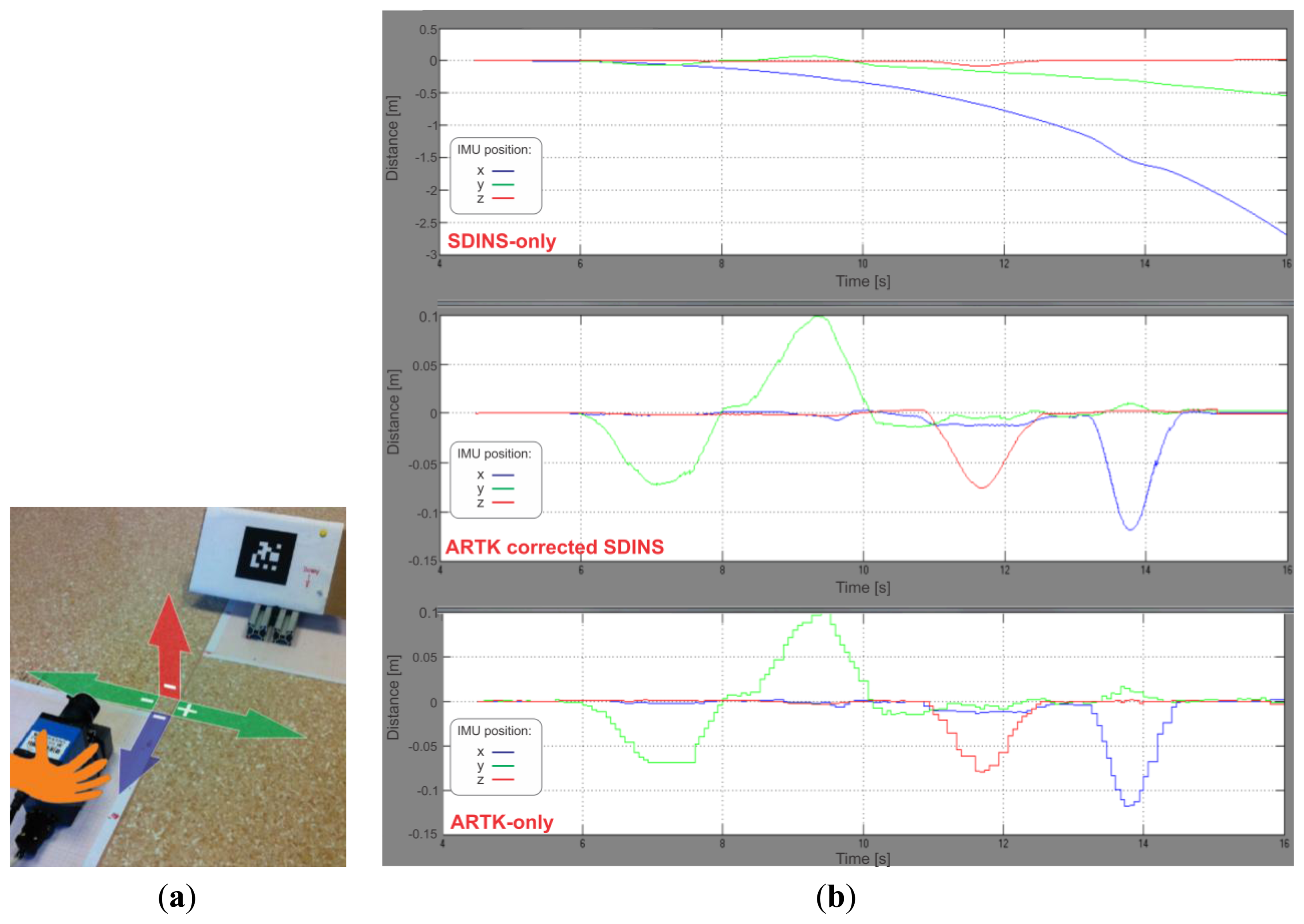
Not having a 3D position measurement device at hand, we first decided to check the behaviour of our system by executing a round trip sequence (i.e., always returning to the starting point) of movements—left, right, up and backward—with the IMU-camera unit in hand, while having the marker in a fixed, tilted position on the floor (Figure 6a). The expected result was a smooth (due to the high rate SDINS calculations) and drift-free (due to the drift-free visual measurements) positional trajectory. We focus here on the positional part of the navigation solution since user position is of greater importance than velocity and orientation in a pedestrian navigation system. Figure 6b shows the results of this 11 seconds-lasting experiment. The upper graph depicts the results of the SDINS-only solution, the graph in the middle shows the final result, obtained with our UKF visual sensor fusion technique, while the graph at the bottom represents the positional ARToolKitPlus measurements expressed in the reference navigation frame with the IMU-camera offsets taken into account. As it can be observed from the graphs, x position coordinate (yellow curve) drifted for almost 3 m, while y position coordinate (violet) drifted for approximately 0.5 m in the SDINS-only graph due to inaccurate gravity vector subtraction—compared to the other two graphs, which are drift-free.
4.2. Slow Walking Experiment
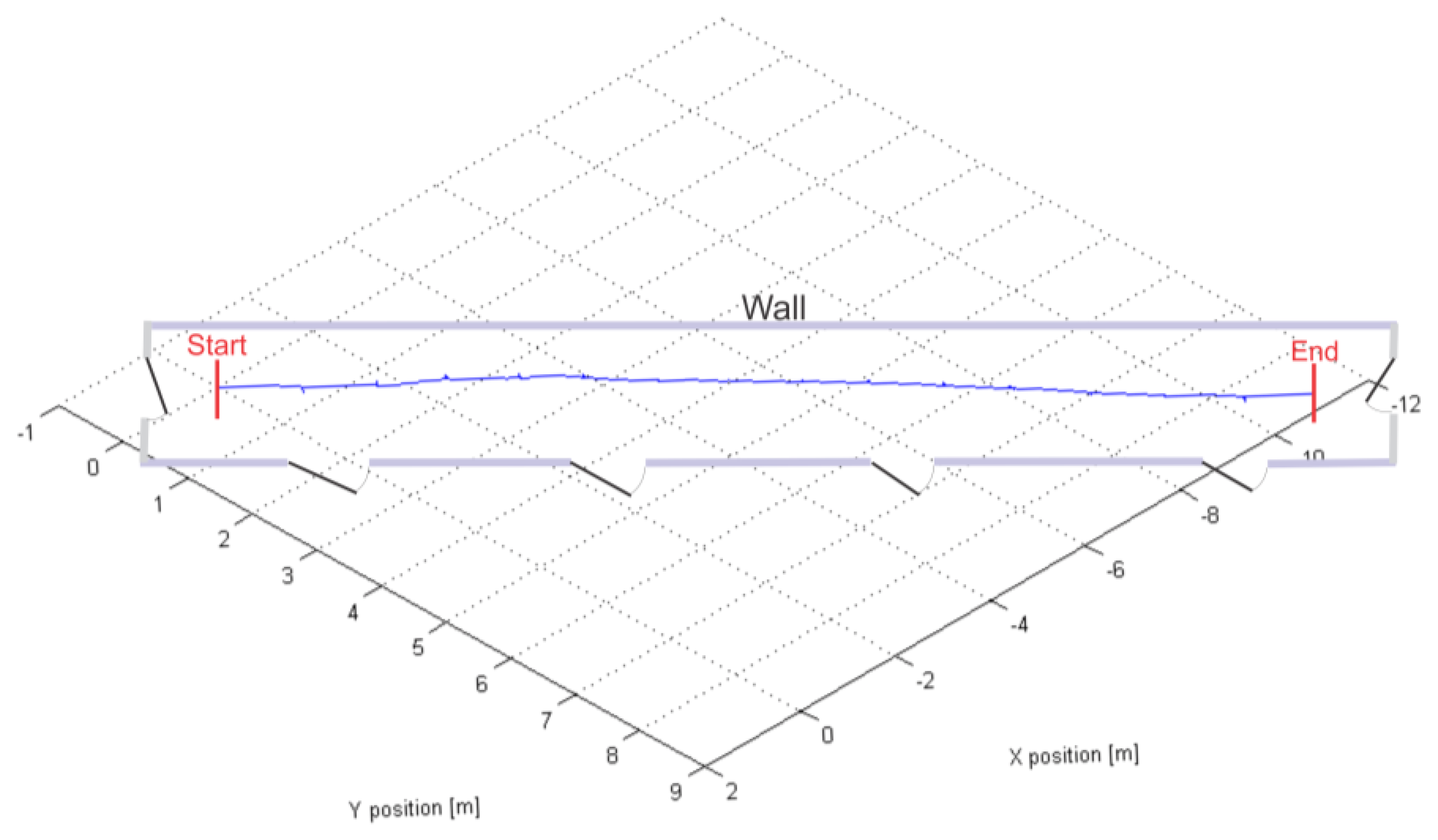
Having checked that the system improves the SDINS-only solution when being used for prolonged periods, we wanted to try it in a real slow walking scenario, to assess the amount of positional error correction during slow paced pedestrian navigation. This second experiment was performed walking slowly down the corridor of our lab, travelling with the IMUCC-equipped foot for 14.09 m in 44 s.
After having preprocessed all the data, ZUPT triggering parameters were set by trial and error:
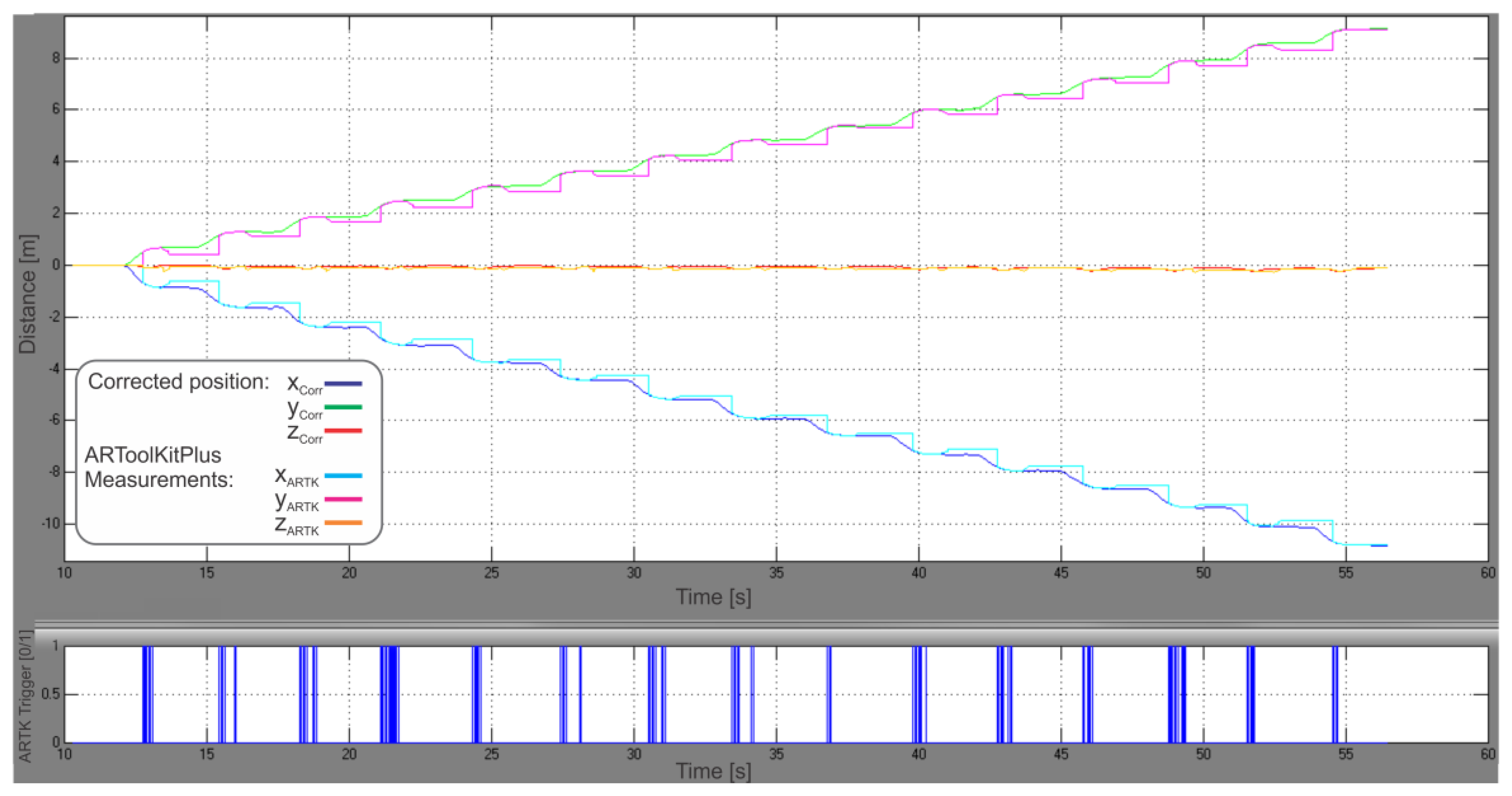
Figure 7 shows the positional graph of our hybrid PDR system with ARTK measurement mode enabled, calculated for the center of the IMU frame in the navigation frame. Fifteen steps done with the IMUCC-equipped foot can be recognized in the upper graph. The x and y position coordinates have a 90° clockwise rotated “V”-letter shape due to the IMUCC significant initial yaw in our experiment, imposed by the desired facing direction of the camera. The z coordinates are negative due to the NED convention employed for the nav-frame. ARTK position measurements were fed to the UKF at the moments, represented by blue spikes in the graph below in Figure 7. The final calculated point in 3D space is 14.15 m distant from the starting point, resulting in a 6 cm (0.43%) travelled distance error. Figure 8 shows the reconstructed experimental slow walk in a 2D top view representation.
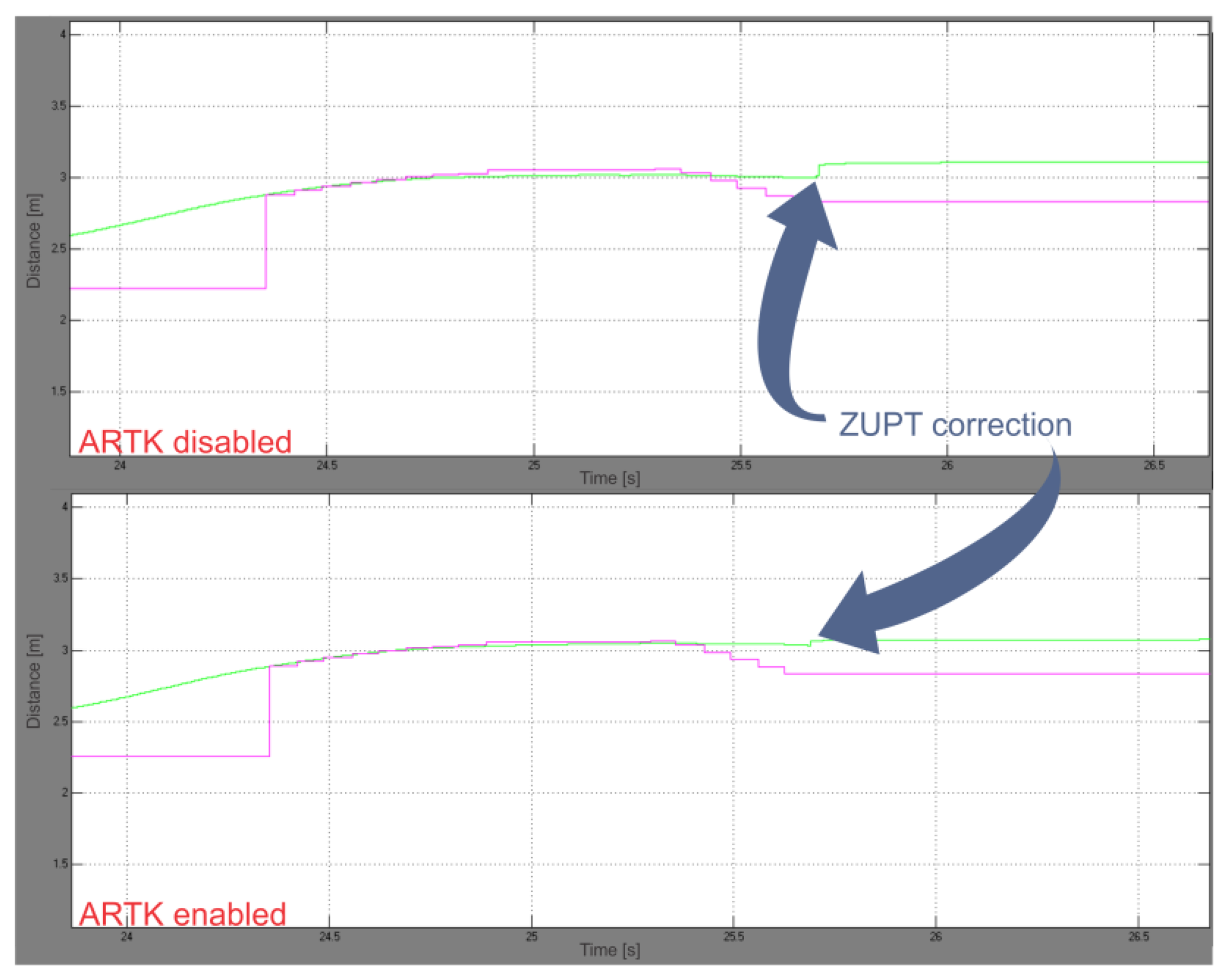
We repeated the calculations on the earlier acquired experimental data with ARTK measurement mode disabled, without altering all the remaining parameters, to be able to compare our proposed solution to a state-of-the-art PDR. A comparison of both positional graphs showed a reduction in ZUPT position corrections in the ARTK-enabled graph (Figure 9).
The upper graph in Figure 10 shows the IMU-frame orientation during the slow walking experiment, while the graph below in Figure 10 depicts the rotational corrections, made by the rotational part of the UKF. Velocity error values, observed for each step at the beginning of the stance phase, just before ZUPT triggering occur, are presented in Table 1. Significant improvement in velocity norm error reduction (25% by comparing the means) is evident from Table 2, where corresponding statistical data is shown.
The final calculated point in 3D space for the ARTK-disabled SDINS system, therefore aided by ZUPT and compass measurements only, is 14.36 m distant from the starting point, resulting in a 27 cm (1.92%) travelled distance error. Comparing it to the 6 cm error with ARTK mode enabled, an 78% increase in accuracy can be observed in our slow walking experiment with our proposed hybrid PDR system.
5. Discussion
A significant improvement (25%) in velocity estimation has been observed during the experiments through beginning-of-stance-phase data analysis (Figure 9), where smaller ZUPT position corrections were observed in the ARTK-enabled graph, which meant greater velocity vector accuracy was achieved during vision-aided navigation. The improvement in velocity vector estimation is the result of a more efficient gravity vector subtraction, i.e., better IMU-frame orientation estimation made possible by ARTK visual position measurements through the correlations developed in the UKF error states covariance matrix. The operational correctness of the rotational part of the filter can be observed also through the last two graphs on Figure 6b, where a great improvement in curve smoothness can be noted in the UKF graph compared to the sole ARToolKitPlus measurements, due to the IMU high sample rate and proper orientation states correction performed by the rotational part of the UKF.
We would like to stress the fact that navigation accuracy improvement is expected to be inversely proportional to the pace of the user and that we have chosen to test our system in a slow pace walk because it would represent a plausible, real-use scenario in which a substantial improvement in navigation accuracy would arise. Conversely, in a normal or fast pace walking, less or even no improvement is expected, due to the shorter SDINS integration time during swing phase. Moreover, using the same visual setup, image blurring would also occur due to the higher camera travel speed, making marker pose estimation less accurate. The mentioned effects of walking speed on accuracy improvement could therefore constitute the subject of further experimental investigation.
Besides walking speed, there is another limitation of our system—the fact that our visual aiding algorithm is based on the assumption of a stationary marker during stance phase of the marker-equipped foot. In fact, any movement of the marker would compromise the visual pose measurement of the marker and consequently the calculated pose of the camera. By examining the video acquired during our experimental walking, we could confirm that we succeeded in achieving no visible marker motion during the experiments in our controlled laboratory environment. However, if intended to be brought to practical use, the system should incorporate some kind of marker movement detection or limitation at least.
6. Conclusions
A proof-of-concept hybrid, inertial sensors-based indoor PDR system, aided by a novel position measurement technique, relying on a shoe-attached marker, has been proposed in this paper. Using a visual marker in this novel way was expected to enhance the navigation solution of an inertial-only PDR, while retaining independence from environmental markers or features, making the proposed approach potentially interesting, especially for first responders' tasks. However, additional sensors could be added to our system in cases when other sensory modalities would be available.
Since a comparison to other indoor pedestrian navigation systems, relying on external aids (e.g., environmental markers, radio fingerprinting, etc.) or environmental assumptions (straight walls, flat floor, ramps, etc.) would not be fair, we compared our system to an inertial PDR aided by ZUPT pseudo-measurements only, where an 78% reduction in error of calculated travelled distance has been shown during an indoor slow walking scenario in the experimental section, while a positioning improvement of 2.7 m was achieved in the axis with major positional error after just 11 s during the preliminary experiment using a marker placed on the floor. All the improvements have been achieved despite no modifications to the environment were made, no a priori knowledge about the environment was presupposed and with the only assumption being that about the marker being stationary during the stance phase of the marker-equipped foot.
Being proof-of-concept, our proposed hybrid PDR cannot be directly used in practice. However, in this paper we have shown that if brought to real-time operation and to a practically acceptable size and weight, the use of a hybrid PDR, aided by visual positional measurements, relying on a shoe-worn marker, can represent a viable solution for improving indoor PDR navigation for first responders in the first place.
Acknowledgments
This research has been co-financed by the European Union—European Social Fund and Slovenian research agency—ARRS, under grants P2-0095, P2-0098 and J2-4284.
Conflict of Interest
The authors declare no conflict of interest.
Appendix: SDINS in Quaternion Approach
The SDINS is the main navigation algorithm in our system, based on IMU outputs. The SDINS algorithm takes IMU-measured accelerations (specific forces) ab=[ax, ay, az] and angular rates in the b-frame with respect to the i-frame and outputs the navigation data (velocity vp, position rp and attitude ) in the p-frame, given the initial velocity, position and attitude. For attitude representation different parametrization options exist—Euler angles, DCM (Direction Cosine Matrix), modified Rodrigues parameters, quaternions and rotation vectors. We have chosen the quaternion approach since it is stated to be computationally effective and avoids singularity problems [25]. We define the SDINS equations in continuous total state space as:
In Equation (A.1) we intentionally ignored the Coriolis and Earth curvature effect part in velocity computation since we use a consumer grade IMU in low dynamics conditions over limited distances making these effects drop below the IMU noise level.
Before using the IMU ab and measurements, raw accelerometer and gyro data have to undergo some preprocessing to assess the turn-on biases. We used mean raw accelerometer data, collected during a stationary stage to calculate roll and pitch and perform leveling—determining the direction cosine matrix DCMinit, describing the initial IMU attitude with respect to the navigation frame through gravity acceleration vector rotation:
Generally, Earth rate is used to derive gyros' turn-on biases, but using a low-cost category IMU this term can be ignored and applying simple mean removal leads to turn-on bias-free data, which can be directly used for navigation.
References
- Curran, K.; Furey, E.; Lunney, T.; Santos, J.; Woods, D.; McCaughey, A. An evaluation of indoor location determination technologies. J. Locat. Based Serv. 2011, 5, 61–78. [Google Scholar]
- Beauregard, S. Omnidirectional Pedestrian Navigation for First Responders. Proceedings of the 4th Workshop on Positioning, Navigation and Communication, WPNC ′07, Hannover, Germany, 22 March 2007; pp. 33–36.
- Ojeda, L.; Borenstein, J.; Gerhart, G.R.; Gage, D.W.; Shoemaker, C.M. Non-GPS navigation with the personal dead-reckoning system. Proc. SPIE 2007, 6561. [Google Scholar] [CrossRef]
- Rantakokko, J.; Händel, P.; Fredholm, M.; Marsten-Eklöf, F. User Requirements for Localization and Tracking Technology: A Survey of Mission-Specific Needs and Constraints. Proceedings of the International Conference on Indoor Positioning and Indoor Navigation (IPIN 2010), Zürich, Switzerland, 15–17 September 2010; pp. 1–9.
- Foxlin, E. Motion Tracking Requirements and Technologies. In Handbook of Virtual Environment Technology; Lawrence Erlbaum: Hillsdale, NJ, USA, 2002; Chapter 7; pp. 163–210. [Google Scholar]
- Rose, J.; Gibson, Gamble J. Human Walking; Lippincott Williams & Wilkins: Philadelphia, PA, USA, 1981; p. 26. [Google Scholar]
- Foxlin, E. Pedestrian tracking with shoe-mounted inertial sensors. IEEE Comput. Graph. Appl. 2005, 25, 38–46. [Google Scholar]
- Alvarez, J.C.; Alvarez, D.; López, A.; González, R.C. Pedestrian navigation based on a waist-worn inertial sensor. Sensors 2012, 12, 10536–10549. [Google Scholar]
- Liu, H.; Darabi, H.; Banerjee, P.; Liu, J. Survey of wireless indoor positioning techniques and systems. IEEE Trans. Syst. Man Cybern. C 2007, 37, 1067–1080. [Google Scholar]
- Corke, P.; Lobo, J.; Dias, J. An introduction to inertial and visual sensing. Int. J. Rob. Res. 2007, 26, 519–535. [Google Scholar]
- Morrison, A.; Renaudin, V.; Bancroft, J.B.; Lachapelle, G. Design and testing of a multi-sensor pedestrian location and navigation platform. Sensors 2012, 12, 3720–3738. [Google Scholar]
- Do, T.N.; Suh, Y.S. Gait analysis using floor markers and inertial sensors. Sensors 2012, 12, 1594–1611. [Google Scholar]
- Wagner, D.; Schmalstieg, D. ARToolKitPlus for Pose Tracking on Mobile Devices. Proceedings of the 12th Computer Vision Winter Workshop (CVWW′07), St. Lambrecht, Austria, 6–8 February 2007.
- Schweighofer, G.; Pinz, A. Robust pose estimation from a planar target. IEEE Trans. Pat. Anal. Mach. Int. 2006, 28, 2024–2030. [Google Scholar]
- Bouguet, J.-Y. Camera Calibration Toolbox for Matlab, 2010. Available online: http://www.vision.caltech.edu/bouguetj/calib_doc/download/index.html (accessed on 11 July 2011).
- Abawi, D.F.; Bienwald, J.; Dörner, R. Accuracy in Optical Tracking with Fiducial Markers: An Accuracy Function for ARToolKit. Proceedings of the International Symposium on Mixed and Augmented Reality, ISMAR, Washington, DC, USA, 2–5 November 2004; pp. 260–261.
- Pentenrieder, K.; Meier, P.; Klinker, G. Analysis of Tracking Accuracy for Single-Camera Square-Marker-Based Tracking. Proceeding of the Third Workshop on Virtual and Augmented Reality of the GI-Fachgruppe AR/VR, Koblenz, Germany, 26 September 2006.
- Hol, J.D.; Schön, T.B.; Gustafsson, F. A New Algorithm for Calibrating a Combined Camera and IMU Sensor Unit. Proceedings of the International Conference on Control, Automation, Robotics and Vision, ICARCV, Hanoi, Vietnam, 17–20 December 2008.
- Van der Merwe, R.; Wan, E.; Julier, S. Sigma-Point Kalman Filters for Nonlinear Estimation and Sensor-Fusion: Applications to Integrated Navigation. Proceedings of the AIAA Guidance, Navigation, and Control Conference and Exhibit, Providence, RI, USA, 16–19 August 2004.
- Wan, E.A.; van der Merwe, R. The Unscented Kalman Filter. In Kalman Filtering and Neural Networks; John Wiley & Sons, Inc.: New York, NY, USA, 2002; pp. 221–280. [Google Scholar]
- John, L.; Crassidis, F.L.M. Unscented filtering for spacecraft attitude estimation. J. Guid. Control Dyn. 2003, 26, 536–542. [Google Scholar]
- Gramkow, C. On averaging rotations. Int. J. Comput. Vision 2001, 42, 7–16. [Google Scholar]
- Cheon, Y.-J.; Kim, J.-H. Unscented Filtering in a Unit Quaternion Space for Spacecraft Attitude Estimation. Proceedings of the IEEE International Symposium on Industrial Electronics, ISIE 2007, Vigo, Spain, 4–7 June 2007; pp. 66–71.
- Kraft, E. A Quaternion-Based Unscented Kalman Filter for Orientation Tracking. Proceedings of the Sixth International Conference of Information Fusion, Cairns, Queensland, Australia, 8–11 July 2003; pp. 47–54.
- Chou, J. Quaternion kinematic and dynamic differential equations. IEEE Trans. Robot. Autom. 1992, 8, 53–64. [Google Scholar]


| Step # | Velocity Vector Norm Error (m/s) with ARTK Disabled | Velocity Vector Norm Error (m/s) with ARTK Enabled |
|---|---|---|
| 1 | 0.1144 | 0.0294 |
| 2 | 0.0872 | 0.0892 |
| 3 | 0.0980 | 0.0608 |
| 4 | 0.0325 | 0.0769 |
| 5 | 0.1293 | 0.0642 |
| 6 | 0.0736 | 0.0283 |
| 7 | 0.0533 | 0.0442 |
| 8 | 0.0713 | 0.0623 |
| 9 | 0.0914 | 0.0747 |
| 10 | 0.0793 | 0.0670 |
| 11 | 0.1030 | 0.0826 |
| 12 | 0.0463 | 0.0195 |
| 13 | 0.0617 | 0.0725 |
| 14 | 0.0294 | 0.0270 |
| 15 | 0.0604 | 0.0533 |
| ARTK Disabled | ARTK Enabled | |
|---|---|---|
| Mean of velocity vector norm error (m/s) | 0.0754 | 0.0568 |
| Standard deviation of velocity vector norm error (m/s) | 0.0291 | 0.0222 |
| Minimum value of velocity vector norm error (m/s) | 0.0294 | 0.0195 |
| Maximum value of velocity vector norm error (m/s) | 0.1293 | 0.0892 |
© 2013 by the authors; licensee MDPI, Basel, Switzerland. This article is an open access article distributed under the terms and conditions of the Creative Commons Attribution license (http://creativecommons.org/licenses/by/3.0/).
Share and Cite
Placer, M.; Kovačič, S. Enhancing Indoor Inertial Pedestrian Navigation Using a Shoe-Worn Marker. Sensors 2013, 13, 9836-9859. https://doi.org/10.3390/s130809836
Placer M, Kovačič S. Enhancing Indoor Inertial Pedestrian Navigation Using a Shoe-Worn Marker. Sensors. 2013; 13(8):9836-9859. https://doi.org/10.3390/s130809836
Chicago/Turabian StylePlacer, Mitja, and Stanislav Kovačič. 2013. "Enhancing Indoor Inertial Pedestrian Navigation Using a Shoe-Worn Marker" Sensors 13, no. 8: 9836-9859. https://doi.org/10.3390/s130809836
APA StylePlacer, M., & Kovačič, S. (2013). Enhancing Indoor Inertial Pedestrian Navigation Using a Shoe-Worn Marker. Sensors, 13(8), 9836-9859. https://doi.org/10.3390/s130809836