Evaluation of Piecewise Polynomial Equations for Two Types of Thermocouples


Abstract
: Thermocouples are the most frequently used sensors for temperature measurement because of their wide applicability, long-term stability and high reliability. However, one of the major utilization problems is the linearization of the transfer relation between temperature and output voltage of thermocouples. The linear calibration equation and its modules could be improved by using regression analysis to help solve this problem. In this study, two types of thermocouple and five temperature ranges were selected to evaluate the fitting agreement of different-order polynomial equations. Two quantitative criteria, the average of the absolute error values |e|ave and the standard deviation of calibration equation estd, were used to evaluate the accuracy and precision of these calibrations equations. The optimal order of polynomial equations differed with the temperature range. The accuracy and precision of the calibration equation could be improved significantly with an adequate higher degree polynomial equation. The technique could be applied with hardware modules to serve as an intelligent sensor for temperature measurement.1. Introduction
Temperature measurement is basic and important work in a variety of industries. Electrical temperature sensors included resistive temperature detectors, thermistors and thermocouples [1,2]. Because of their multiple advantages of low cost, robustness and easily standardization, thermocouples are the most frequently used sensors for temperature measurement. They can measure a wide range of temperatures and have long-term stability and high reliability [3,4]. However, the major problems of this sensor for signals conditioning are the cold junction compensation and linearization of the transfer relationship between temperature and output voltage [2,3].
Output voltage tables for various types of thermocouples list the output voltage corresponding to different temperatures [5]. The reference junction is fixed at 0 °C. The relation between output voltage and temperature is established as a higher order polynomial equation for each type thermocouple [1,3]. For T-type thermocouples, the relation equation is an 8th order polynomial equation for the temperature range from 0–400 °C. For practical applications, this calibration equation is expressed as an inverse equation. Temperature is recognized as the dependent variable and the output voltage serves as the independent variable.
Because these calibration equations are higher order polynomial equations, Sarma and Boruan [6] suggested that the whole temperature range can be divided into smaller ranges, with lower degree polynomial calibrations being used for each range [4], but the literature contains no reports of any applications of this method.
Hardware modules have been designed to linearize the non-linear signals with hardware linearization [7]. The curve of nonlinear signals was divided into several pieces. The relationship between input and output was assumed to be a linear equation. The thermocouple input signal for each piece was filtered, isolated, amplified and converted to an analog voltage output by a linear equation [6].
The theory of the calibration with piecewise linear regression has been discussed [8]. Several self-compensation methods were proposed to build reconfigurable measurement systems for designing intelligent sensors [9]. The thermistor output from 0 °C to 100 °C was selected to compare errors of the measurement system. However, the piecewise linear interpolation method had the largest errors for these methods.
Some generalized software techniques for linearisation transducers had been used for thermocouples [10,11]. However, their performances have seldom been reported. An increase in table size of the thermocouple output voltage could improve the accuracy, but is impractical for an electrical thermometer. More electronic circuits for linearization could enhance the accuracy. However, these circuits are affected by ambient temperature, electromagnetic, and radiofrequency interference [10,11]. A log-amplifier based circuit for linearizing thermocouple signals was described [12]. Three types of thermocouples were selected to compare simulation results. The maximum percentage nonlinearity error before and after linearization were reduced significantly. To design a higher precision industrial temperature measurement system, Sarma et al. [13] linearized the amplified thermo-emf of a K-type thermocouple with the least squares polynomial fitting technique. Four temperature ranges were selected. The parameters for linear and polynomial equations were estimated for receiving signals gained by the amplifier and the accuracy was better with polynomial equations than linear fitting.
Sarma and Boruan [6] developed a measurement system for a K-type thermocouple with analog-to-digital converter, amplifier reference junction and computer. The measurement temperature range was 0 °C to 200 °C. Two calibration equations, a 9th order polynomial and a linear model, were proposed by a least squares method. The accuracy was within ±0.08 °C at 100.2 °C standard temperature. The authors suggested that the precision could be improved with a higher order regression equation, but did not report their adequate regression model. Danisman et al. [14] designed a high precision temperature measurement system based on an artificial neural network for three types of thermocouples. A neural linearizer was used to compute the temperature from the output voltage of the thermocouples.
For determining the optimal order of polynomial equations for temperature measurement, data fitting ability and prediction performance are both important [15]. A higher order polynomial equation has higher values for the coefficient of determination (R2). However, the standard values of estimation could be increased with the loss of data freedom. A higher degree polynomial equation may be over-fitted and the predicted ability thus decreased [16]. Resistance-temperature calibration equations for a negative temperature coefficient (NTC) thermistor have been evaluated with a modern regression technique to show the importance of an adequate calibration equation [16]. The division of the whole measurement range into smaller temperature ranges was proposed [6]. These calibration equations could be transformed with the use of software and incorporated into an intelligent sensor.
In the previous studies, the curves of the relationship of temperature and output voltage were divided into many pieces. Each piece of these curves was assumed as a linear relationship, however, the residual plots of each piece still indicated nonlinear results [4,7,13]. The linear equation should not be the only choice for establishing of calibration equations. Least squares-based parabolic regression had been reported to determine the parameters of the calibration equation [17]. As the piece relationship between temperature and output voltage of a thermistor was assessed with the 4th order polynomial equation, the accuracy and precision could be improved significantly [16].
In this study, the data of output voltage for two types of thermocouple were used from the US National Institute of Standards and Technology (NIST) standard. Five temperature ranges were selected to evaluate their calibration polynomial equations, called piecewise polynomial equations. The parameters for these equations were estimated by the least squares technique. The fitting performance of these equations was evaluated by several statistical methods.
2. Calibration Equations
2.1. Calibration Equations
The inverse calibration equation was used to describe the relationship between temperature (T) and output voltage of thermocouples (mv). Because the output voltage at 0 °C for thermocouples is zero, the intercept is excluded in a polynomial equation:
2.2. Temperature-Voltage Data of Thermocouples
Table data for thermocouples [5] were selected to evaluate the fitting ability of the calibration in this study.
2.2.1. Type of Thermocouples: T-Type and J-Type
Two-types of thermocouples were selected in this study for their popularity in industry. The method developed in this study could be used for other thermocouples. The J-type thermocouple is commonly used for higher temperature ranges. In this study, the type of thermocouple was selected to evaluate the improved performance by piecewise polynomial equation.
2.2.2. Piecewise Range of Temperature
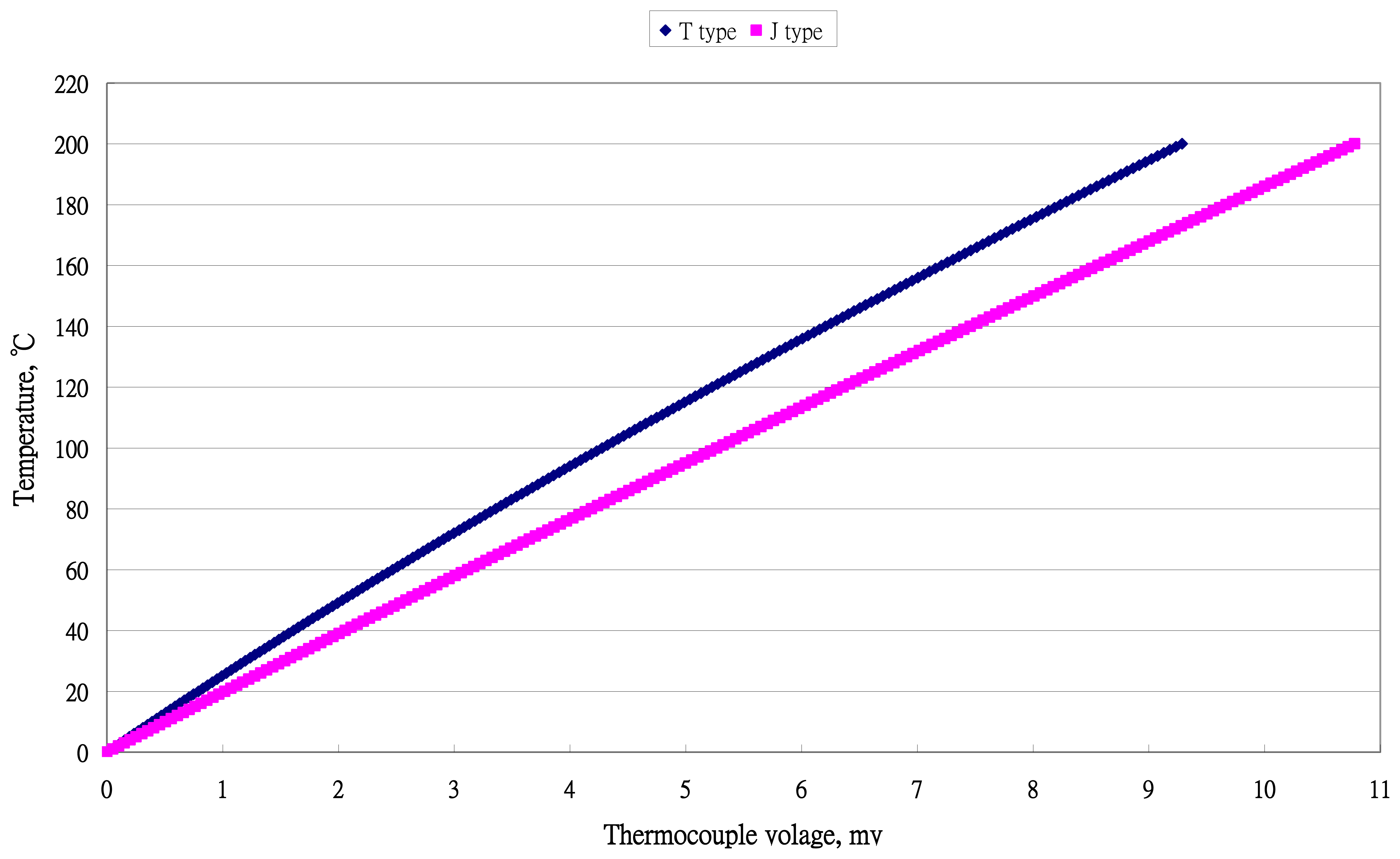
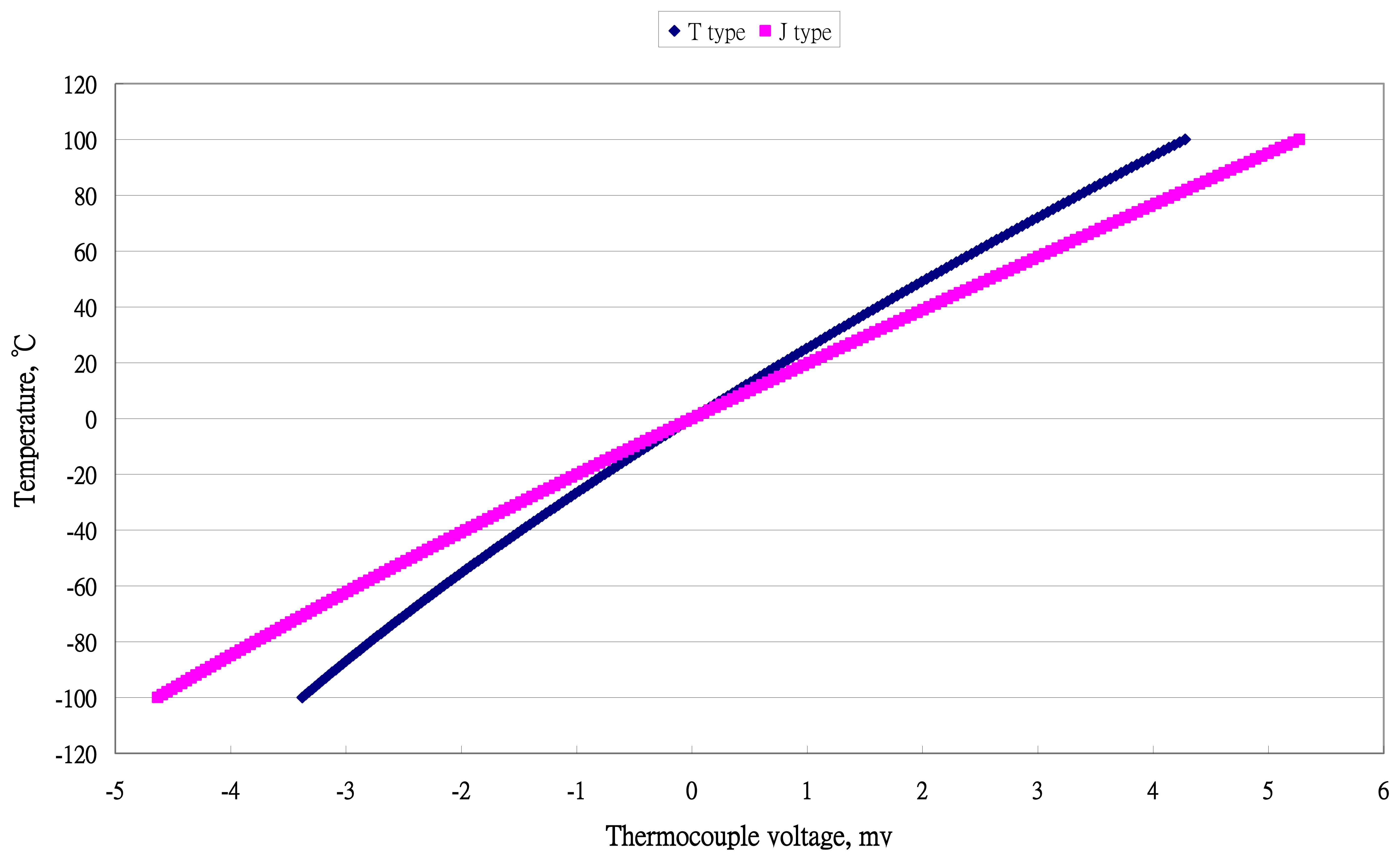
There were five ranges (a) 0∼100 °C; (b) 0∼200 °C; (c) −50∼50 °C; (d) −100∼0 °C; and (e) −100∼100 °C. They are the ranges for most living systems, included human beings. The distribution of temperature data for temperature versus voltage for two types of thermocouples are presented in Figures 1 and 2.
2.3. Data Analysis
Microsoft Excel 2003 was used to estimate the parameters of the different order polynomial equations. The t value of the highest order parameter was used to evaluate the optimal order of polynomial equations. If the order of polynomial equation is underestimated, the estimated parameters and variance will have a fixed bias. If the order of polynomial equation is overestimated, the variance increases and the bias of the prediction ability will inflate [6,15]. Residual plots were used as the qualitative criterion to evaluate the adequateness of models [15]. If the model is adequate for expressing the relationship between independent and dependent variables, the error distribution in residual plots is represented as horizontal bands. If the model is not adequate, the residual plots show a clear systematic pattern. The error was defined as follows:
Three statistics, emax, emin and |e|ave were used as quantitative criteria. The emax is the maximum ei value, emin is the minimum ei value and |e|ave is the average of the absolute errors:
The other criterion for uncertainty comparing of calibration equations is precision. The precision performance could be calculated from the standard deviation of the calibration equation [18]:
3. Evaluation of Calibration Equations of Thermocouples
3.1. T-Type Thermocouple
The estimated parameters of calibration equations for five temperature ranges are listed in Table 1. The quantitative criteria for these calibration equations are listed in Tables 2 and 3.
3.1.1. Range 0∼100 °C
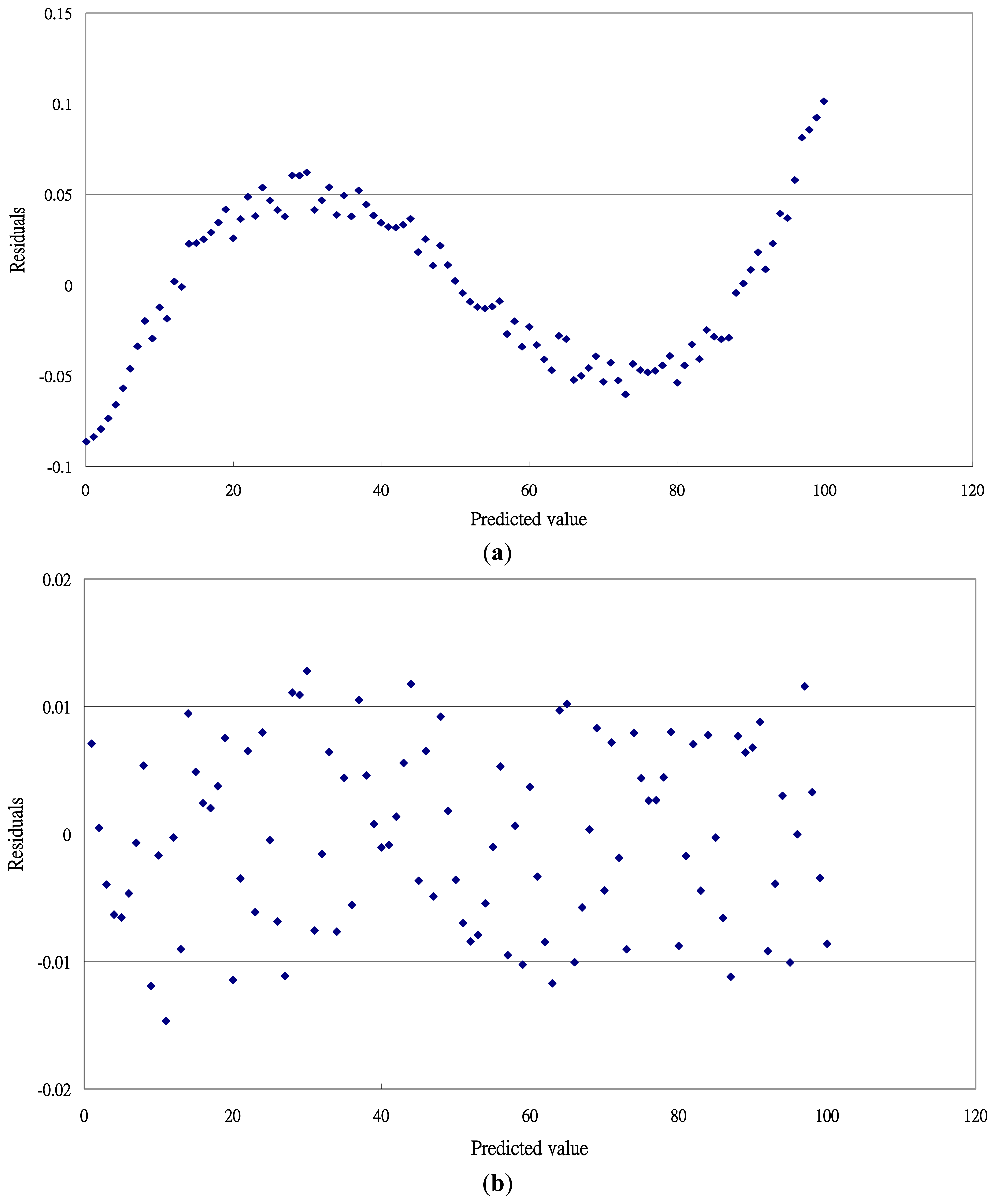
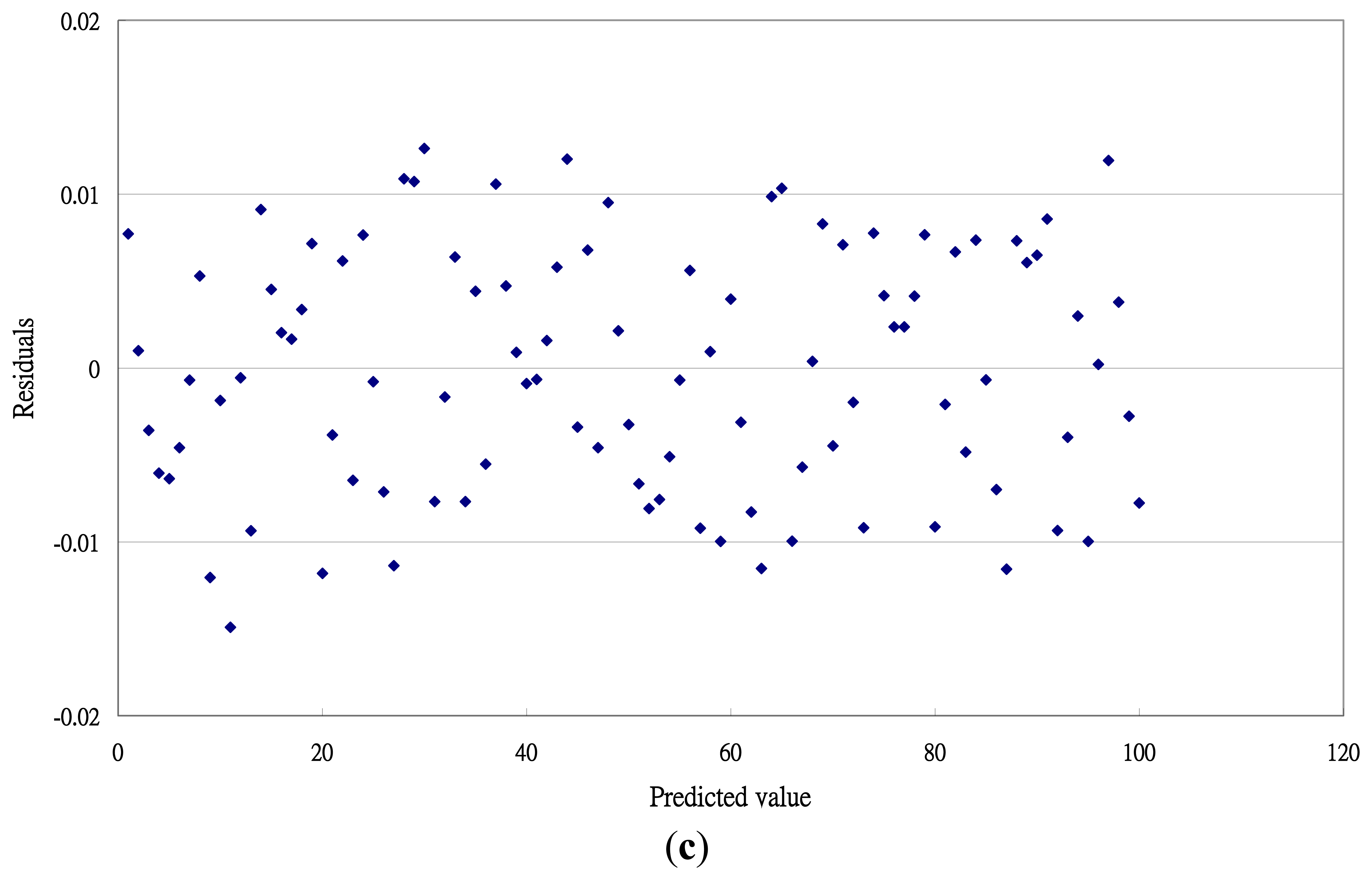
The 2nd order polynomial equation produced a clear systematic pattern of residual plots (Figure 3a). The 3rd and 4th order polynomial equations produced a random distribution on residual plots (Figure 3b and c). Thus, the 2nd polynomial equation was not adequate because of systematic errors were found over the temperature ranges.
The |e|ave value represents the accuracy of the calibration equation. From Table 2, the 2nd order polynomial equation had the largest value for emax, emin and |e|ave. The |e|ave values for the 3rd and 4th order polynomial equations did not differ substantially: 0.00681306 and 0.00676768, respectively.
The estd value represents precision of the calibration equation. The estd values for the 2nd, 3rd and 4th order polynomial equations were 0.05325660, 0.00840050 and 0.00824098, respectively (Table 3). The reduction in estd values between 2nd and 3rd order polynomial equation was about 1/6.5 but that between 3rd and 4th order polynomial equations was not substantial. The increase in the 4th order (c4x4) of the calibration equation had only a marginal effect on improving performance. The adequate calibration equation for the T-type thermocouple for temperature 0 to 100 °C is as follows:
3.1.2. Range 0∼200 °C
The 2nd and 3rd order polynomial equations produced a systematic residual pattern and 4th and 5th order polynomial equations revealed a uniform distribution. All residual figures were showed in Supplement Figures A.
The |e|ave values for the 2nd, 3rd, 4th and 5th order polynomial equations were 0.36507503, 0.03911083, 0.00718054 and 0.00680437, respectively (Table 2). Therefore, the 4th and 5th degree equations had the best accuracy.
The estd values for the above four equations were 0.41512994, 0.04580101, 0.00940073 and 0.00860020, respectively (Table 3). Comparing 3rd degree equation with 4th degree equation, the reduction in estd value between 3rd and 4th order equation was approximately 1/5. Comparing with the 4th order equation, the contribution of the 5th order equation was substantial. The reduction in precision was limited. Therefore, the adequate equation for the T-type thermocouple for temperature 0 to 200 °C is as follows:
3.1.3. Range −50∼50 °C
This temperature range included the activity environment for the most biological system. The residual plots of the 2nd, 3rd and 4th order calibration equations are presented in Supplement Figure B. Only the 4th order equation showed a random distribution in residual plot. The 4th order polynomial had the smallest |e|ave and estd values (Tables 2 and 3). The following equation was considered as adequate:
3.1.4. Range −100∼0 °C
Only the 4th order polynomial equation had a uniform distribution on residual plots (data not shown) and the smallest value of |e|ave and estd (Tables 2 and 3). This following equation was considered adequate:
3.1.5. Range −100∼100 °C
The shape of the data distribution between temperature and thermocouple output voltage is a nonlinear curve. Only a higher order polynomial equation could produce a uniform distribution on residual plot (data not shown). The adequate calibration equation was a 6th order polynomial equation and showed as follows:
The |e|ave value represents the accuracy and the estd value was used to assess the precision of these equations. By the selection of the adequate polynomial calibration equations, the |e|ave was < 0.009 °C and the estd value was < 0.012 °C for the T-type thermocouple.
3.2. J-Type Thermocouple
The estimated parameters for calibration equations for five temperature ranges are listed in Table 4 and the quantitative criteria are listed in Tables 5 and 6.
All datasets for different temperature ranges were evaluated by regression analysis. The residual plots were used to evaluate the adequateness of models. The |e|ave and estd values were used to assess accuracy and precision. The adequate equations for different temperature ranges are listed as follows:
- (1)
1.0∼100 °C
- (2)
0∼200 °C
- (3)
−50∼50 °C
- (4)
−100∼0 °C
- (5)
−100∼100 °C
With the selection of the adequate polynomial calibration equations, the |e|ave was <0.005 °C and The estd value was <0.008 °C for the J-type thermocouple. The |e|ave value presented the accuracy and the estd value showed the precision of these equations. These numeric values indicated the performance improvement for this type thermocouple using in the special temperature range.
Now, the development of microprocessor systems is rapid and the price is dwindling. The nonlinear characteristics of sensing element could be improved by software package techniques. The calculation of the higher order polynomial equation could be treated as rapidly and accurately as linear equations. In this study, the orders of their polynomial equations for adequate calibration equations were lower than that of the NIST Standards. The accuracy and precision of these equations were improved significantly compared to that of a linear equation. They could be adapted to microprocessor systems to enhance the measurement performance of different types of thermocouples. The suggestion of the application of these polynomial calibration equations are as follows:
The analog mv output of the thermocouple is amplified to voltage.
The voltage signal is digitized by A/D converter.
The function of the A/D converter is controlled by a microcomputer.
The software for these calibrations is embedded in the flash ROM of the microcomputer.
The true temperature then is computed by its adequate polynomial calibration equation.
The true temperature could be display in a LCD or send to a PC via RS232 for data display or send to temperature controller.
4. Conclusions
Thermocouples are the most frequently used sensors for temperature measurement. However, linearizing the transfer relationship between temperature and output voltage is one of their major problems. In this study, two types of thermocouple with five temperature ranges were selected to evaluate the fitting agreement of different order polynomial equations to help solve this problem. The estimated parameters were established by regression analysis techniques. Two quantitative criteria, |e|ave and estd were used to evaluate the accuracy and precision of these calibrations equations. Residual plots were applied to justify the adequateness of these models.
The adequate order of polynomial calibration equation was affected by the temperature range. The 3rd order polynomial equation was adequate for the 0 to 100 °C temperature range and the higher 6th order polynomial equation was adequate for the −100 °C to 100 °C range.
The |e|ave value represents the accuracy of these equations. The estd value was used to assess the precision of equations. With the adequate polynomial calibration equation, the |e|ave was <0.009 °C for the T-type thermocouple and <0.005 °C for the J-type thermocouple. The numeric value of estd was <0.012 °C for the T-type thermocouple and <0.008 °C for the J-type thermocouple.
These polynomial calibration equations are easy to be written as software and be incorporated into an IC circuit as calculated equations. The measured thermocouple output could be transformed into the temperature easily and accurately. The technique could be applied with hard modules to serve as intelligent sensors. The regression analysis technique and criteria for comparison used in this study could be applied to evaluate adequate calibration equations for other thermocouples with different temperature ranges. The piecewise polynomial equation could be established to meet the requirement temperature range for practical applications.
Acknowledgments
The authors would like to thank the National Science Council of the Republic of China for financially supporting this research under Contract No. 98-2313-B-005-032-MY3.
Conflicts of Interest
The authors declare no conflict of interest.
References
- Nicholas, J.V.; White, D.R. Traceable Temperatures; John Wiley & Sons, Inc.: New York, NY, USA, 1994. [Google Scholar]
- Childs, P.R.N.; Greenwood, J.R.; Long, C.A. Review of temperature measurement. Rev. Sci. Instrum. 2000, 71, 2959–2978. [Google Scholar]
- Kerlin, T.W.; Joshson, M. Practical Thermocouple Thermometry, 2nd ed.; ISA Publisher: New York, NY, USA, 2012. [Google Scholar]
- Yilmaz, N.; Gill, W.; Donaldson, A.B.; Lucero, R.E. Problems encountered in fluctuating flame temperature measurements by thermocouple. Sensors 2008, 8, 7882–7893. [Google Scholar]
- National Institute of Standards and Testing. Available online: http://srdata.nist.gov/its90/main/ (accessed on 5 December 2013).
- Sarma, U.; Boruah, P.K. Design and development of a high precision thermocouple based smart industrial thermometer with on line linearisation and data logging feature. Measurement 2010, 43, 1589–1594. [Google Scholar]
- Ayman, A.A.; Ei-Lail, A.S.A. A novel circuit for thermocouple signals linearization using AD converter. IJITCS 2013, 3, 56–60. [Google Scholar]
- Ndlovu, P.; Preater, J. Calibration using a piecewise simple linear regression model. Commun. Stat. Theory Method. 2001, 20, 229–242. [Google Scholar]
- Rivera-Mejia, J.; Carrillo-Romero, M.; Herrera-Ruiz, G. Self-compensation to build reconfigurable measurement systems. IEEE Instrum. Meas. Mag. 2013, 16, 10–19. [Google Scholar]
- Patranabis, D.; Ghosh, D.; Bakshi, C. Linearizing transducer characteristics. IEEE Instrum. Meas. Mag. 1988, 37, 66–69. [Google Scholar]
- Ghosh, D.; Patranabis, D. Linearizing of transducers through a generalized software technique. J. Phys. E Meas. Sci. Technol. 1991, 2, 102–105. [Google Scholar]
- Mondal, N.; Abudhahir, A.; Jana, S.K.; Munshi, S.; Bhattacharya, D.P. A log amplifier based linearization scheme for thermocouples. Sens. Transd. 2009, 100, 1–10. [Google Scholar]
- Sarma, U.; Chakraborty, D.; Boruah, P.K. Design of a smart and high precision industrial temperature measurement and monitoring system using K-type thermocouple and SPI-compatible temperature sensor. Sens. Transd. 2009, 102, 1–9. [Google Scholar]
- Danisman, K.; Dalkiran, I.; Celebi, F.V. Design of a high precision temperature measurement system based on artificial neural network for different thermocouple types. Measurement 2006, 39, 696–700. [Google Scholar]
- Myers, R.H. Classical and Modern Regression with Application, 2nd ed.; PWS and Kent Publisher: Boston, MA, USA, 1986. [Google Scholar]
- Chen, C. Evaluation of resistance-temperature calibration equations for NTC thermistors. Measurement 2009, 42, 1103–1111. [Google Scholar]
- Mallick, P.; Nayak, C.; Behera, T.B. Least Square Based Parabolic Regression to Determine Calibration Constant in Measurement. Proceedings of the 5th International Conference on Industrial and Information Systems, Mangalore, India, 29 July–1 August 2010; pp. 334–338.
- Eurachem. EURACHEM/CITAC Guide Quantifying Uncertainty in Analytical Measurement, 3rd ed.; Eurachem: Uppsala, Sweden, 2012. [Google Scholar]


| Equation | bi | 0–100°C | 0–200°C | −50–50°C | −100–0°C | −100–100°C |
|---|---|---|---|---|---|---|
| 2nd order | b1 | 25.67471979 | 25.07879340 | 26.00810515 | −25.22117110 | 26.44647267 |
| b2 | −0.54576494 | −0.39314346 | −0.74516432 | −1.26190490 | −0.78530785 | |
| 3rd order | b1 | 25.86464325 | 25.76378439 | 25.85804386 | −25.90849949 | 25.91435043 |
| b2 | −0.69457635 | −0.64264925 | −0.75808252 | −0.59839052 | −0.83435521 | |
| b3 | 0.026133029 | 0.020317674 | 0.066304477 | −0.14489758 | 0.061098417 | |
| 4th order | b1 | 25.84962602 | 25.09020576 | 25.84551540 | −25.77505075 | 25.81912460 |
| b2 | −0.673394463 | −0.73340079 | −0.70994624 | −0.830585167 | −0.74867280 | |
| b2 | 0.017448349 | 0.037584526 | 0.074689216 | −0.026571395 | 0.077691433 | |
| b4 | −1.082962 × 10⁻³ | −9.9772501 × 10⁻⁴ | −0.018167033 | −0.018427604 | −8.8817640 × 10⁻³ | |
| 5th order | b1 | 25.88262726 | 25.86505358 | |||
| b2 | −0.71357086 | −0.73577069 | ||||
| b2 | 0.031114204 | 0.062941133 | ||||
| b4 | −1.5600801 × 10⁻⁴ | −0.010532441 | ||||
| b5 | 3.7937780 × 10⁻⁵ | 9.7149801 × 10⁻⁴ | ||||
| 6th order | b1 | 25.85453185 | ||||
| b2 | −0.72787713 | |||||
| b2 | 0.067478989 | |||||
| b4 | −0.012651926 | |||||
| b5 | 6.0999501 × 10⁻⁴ | |||||
| b6 | −1.3091201 × 10⁻⁴ |
| Equation | Criteria | 0–100°C | 0–200°C | −50–50°C | −100–0°C | −100–100°C |
|---|---|---|---|---|---|---|
| 2nd order | emin | −0.07447137 | 0.49823066 | 0.225686384 | −0.36968565 | −1.67100581 |
| emax | 0.13074332 | 0.98345135 | 0.13642422 | 0.18487408 | 1.21440524 | |
| |e|ave | 0.04592460 | 0.36507503 | 0.06717221 | 0.12630630 | 0.48771413 | |
| 3th order | emin | −0.02072832 | 0.13412573 | 0.06409870 | −0.04361028 | −0.55185176 |
| emax | 0.01471193 | 0.07282170 | 0.04472070 | 0.03208275 | 0.285123028 | |
| |e|ave | 0.00681306 | 0.03911083 | 0.02223685 | 0.01384381 | 0.150423885 | |
| 4th order | emin | −0.01753270 | 0.03052425 | 0.02023304 | −0.01507971 | −0.07094427 |
| emax | 0.01501541 | 0.19169659 | 0.02069277 | 0.01633248 | 0.11870578 | |
| |e|ave | 0.00676768 | 0.00718054 | 0.00763593 | 0.00663725 | 0.027618094 | |
| 5th order | emin | 0.02534386 | −0.027957131 | |||
| emax | 0.01656904 | 0.03741114 | ||||
| |e|ave | 0.00680437 | 0.01217997 | ||||
| 6th order | emin | -0.02814230 | ||||
| emax | 0.02771649 | |||||
| |e|ave | 0.00986177 |
| Equation | 0–100°C | 0–200°C | −50–50°C | −100–0°C | −100–100°C |
|---|---|---|---|---|---|
| 2nd order | 0.05325659 | 0.41512994 | 0.079658494 | 0.14552443 | 0.57348457 |
| 3rd order | 0.00840050 | 0.04580101 | 0.026619274 | 0.01675441 | 0.18449760 |
| 4th order | 0.00824098 | 0.00940073 | 0.009181103 | 0.00794493 | 0.03658164 |
| 5th order | 0.00860020 | 0.01527604 | |||
| 6th order | 0.01228220 |
| Equation | bi | 0–100°C | 0–200°C | −50–50°C | −100–0°C | −100–100°C |
|---|---|---|---|---|---|---|
| 2nd order | b1 | 19.71440273 | 19.45794480 | 19.92321865 | 19.53896507 | 20.15400867 |
| b2 | −0.14280031 | −0.08790950 | −0.24205613 | −0.42806222 | −0.25366061 | |
| 3rd order | b1 | 19.82859586 | 19.76305984 | 19.84718826 | 19.91333650 | 19.85023043 |
| b2 | −0.21497883 | −0.18247776 | −0.24479520 | −0.16293062 | −0.26518721 | |
| b3 | 0.01024941 | 0.006582481 | 0.019753541 | 0.042391433 | 0.02046607 | |
| 4th order | b1 | 19.84344081 | 19.82989561 | 19.84610586 | 19.83020340 | 19.82940836 |
| b2 | −0.23187152 | −0.21979759 | −0.23898495 | −0.26902673 | −0.23785577 | |
| b3 | 0.01584881 | 0.012647965 | 0.020179476 | 2.9937101 × 10⁻³ | 0.02258792 | |
| b4 | −5.6514610 × 10⁻⁴ | −3.0010410 × 10⁻³ | −1.2941520 × 10⁻³ | −4.5105150 × 10⁻³ | −1.5837460 × 10⁻³ | |
| 5th order | b1 | 19.85185466 | 19.84739765 | |||
| b2 | −0.22599582 | −0.23586796 | ||||
| b3 | 0.030341877 | 0.019194036 | ||||
| b4 | −2.5509630 × 10⁻³ | −1.7327180 × 10⁻³ | ||||
| b5 | 6.2928705 × 10⁻⁴ | 1.2591410 × 10⁻⁴ | ||||
| 6th order | b1 | 19.84959392 | ||||
| b2 | −0.23844914 | |||||
| b3 | 0.018639399 | |||||
| b4 | −1.4776299 × 10⁻³ | |||||
| b5 | 1.5145010 × 10⁻⁴ | |||||
| b6 | −1.2754301 × 10⁻⁵ |
| Equation | Criteria | 0–100°C | 0–200°C | −50–50°C | −100–0°C | −100–100°C |
|---|---|---|---|---|---|---|
| 2nd order | emin | 0.05557809 | 0.24933012 | 0.13616157 | −0.28775249 | −1.18173165 |
| emax | 0.08928586 | 0.47674018 | 0.11595334 | 0.14466809 | 0.85074564 | |
| |e|ave | 0.03400235 | 0.18601820 | 0.04196053 | 0.09499065 | 0.33772693 | |
| 3rd order | emin | 0.01317127 | 0.068261782 | 0.02101240 | −0.04169692 | −0.30645416 |
| emax | 0.01187325 | 0.046436731 | 0.01547939 | 0.02779399 | 0.14204194 | |
| |e|ave | 0.00481871 | 0.021161537 | 0.00574589 | 0.01190433 | 0.07435890 | |
| 4th order | emin | 0.01009384 | 0.013460643 | 0.01074795 | −0.01449671 | -0.06051327 |
| emax | 0.00925146 | 0.013254812 | 0.00786120 | 0.01273097 | 0.03879727 | |
| |e|ave | 0.00429203 | 0.004711247 | 0.00438609 | 0.00532295 | 0.01359488 | |
| 5th order | emin | −0.01239944 | −0.02524355 | |||
| emax | 0.01075262 | 0.01869201 | ||||
| |e|ave | 0.00507465 | 0.00580843 | ||||
| 6th order | emin | −0.01393513 | ||||
| emax | 0.01228582 | |||||
| |e|ave | 0.00482716 |
| Equation | 0–100°C | 0–200°C | −50–50°C | −100–0°C | −100–100°C |
|---|---|---|---|---|---|
| 2nd order | 0.03903280 | 0.21139799 | 0.049680 | 0.10986868 | 0.39874169 |
| 3rd order | 0.00585086 | 0.02519590 | 0.007350308 | 0.01429016 | 0.09409667 |
| 4th order | 0.00522916 | 0.00582213 | 0.005281434 | 0.00641780 | 0.016754189 |
| 5th order | 0.00537354 | 0.00612658 | 0.00723238 | ||
| 6th order | 0.00581152 |
© 2013 by the authors; licensee MDPI, Basel, Switzerland. This article is an open access article distributed under the terms and conditions of the Creative Commons Attribution license (http://creativecommons.org/licenses/by/3.0/).
Share and Cite
Chen, A.; Chen, C. Evaluation of Piecewise Polynomial Equations for Two Types of Thermocouples. Sensors 2013, 13, 17084-17097. https://doi.org/10.3390/s131217084
Chen A, Chen C. Evaluation of Piecewise Polynomial Equations for Two Types of Thermocouples. Sensors. 2013; 13(12):17084-17097. https://doi.org/10.3390/s131217084
Chicago/Turabian StyleChen, Andrew, and Chiachung Chen. 2013. "Evaluation of Piecewise Polynomial Equations for Two Types of Thermocouples" Sensors 13, no. 12: 17084-17097. https://doi.org/10.3390/s131217084
APA StyleChen, A., & Chen, C. (2013). Evaluation of Piecewise Polynomial Equations for Two Types of Thermocouples. Sensors, 13(12), 17084-17097. https://doi.org/10.3390/s131217084