Improving the Responses of Several Accelerometers Used in a Car Under Performance Tests by Using Kalman Filtering

Abstract

In this paper a Kalman filter is used to cancel noise and interference contained in two accelerometers embedded in a car under performance tests. Here, the frequency bands of the signals of interest and their noise (deterministic as well as stochastic) are not strongly mixed with each other but it is very difficult to diminish the noise by using the classical approach to filtering. This reason, among others, justifies the necessity of the application of optimal filtering; and the Kalman filtering application allowed us to obtain optimal results (in the minimum mean-square sense) and signal-to-noise ratio improvements higher than 30 dB were achieved. The experimental results demonstrate the importance of using both analog signal conditioning and digital signal processing when dealing with signals corrupted by noise.

Introduction

Nowadays the automobile is one of our main means of transportation. We make extensive use of it for several purposes throughout our entire lives. So, all the efforts that we currently make oriented to improve its performance and our road safety are few. In this sense a significant part of the increasing developments in microelectronics, sensors, instrumentation, optimal feedback control, etc., has been focused on building cars able to make intelligent driving decisions. For this reason a method for the optimal estimation of several variables of a car under performance tests is used in this paper.

The present paper can be seen as a second part of [1], where a recursive least-squares algorithm (RLS) was used as an adaptive filtering tool to cancel the noise presented in the response of an accelerometer. Here, however, a Kalman filter [2,3,4,5,6,7,8,9] is used for the same purpose and it shows the following additional advantages, among others:

(i)

It is used as an optimal multivariable filter,

(ii)

We do not make use of any noise source for noise canceling purposes,

(iii)

The Kalman filter provides estimates than can be used for advanced feedback control.

In reference [1], a RLS adaptive filter to cancel unknown interference contained in a primary signal was used, with the cancellation being optimized in the minimum mean-square sense of the a priori estimation error between the desired response and the output of the transversal filter used [2].

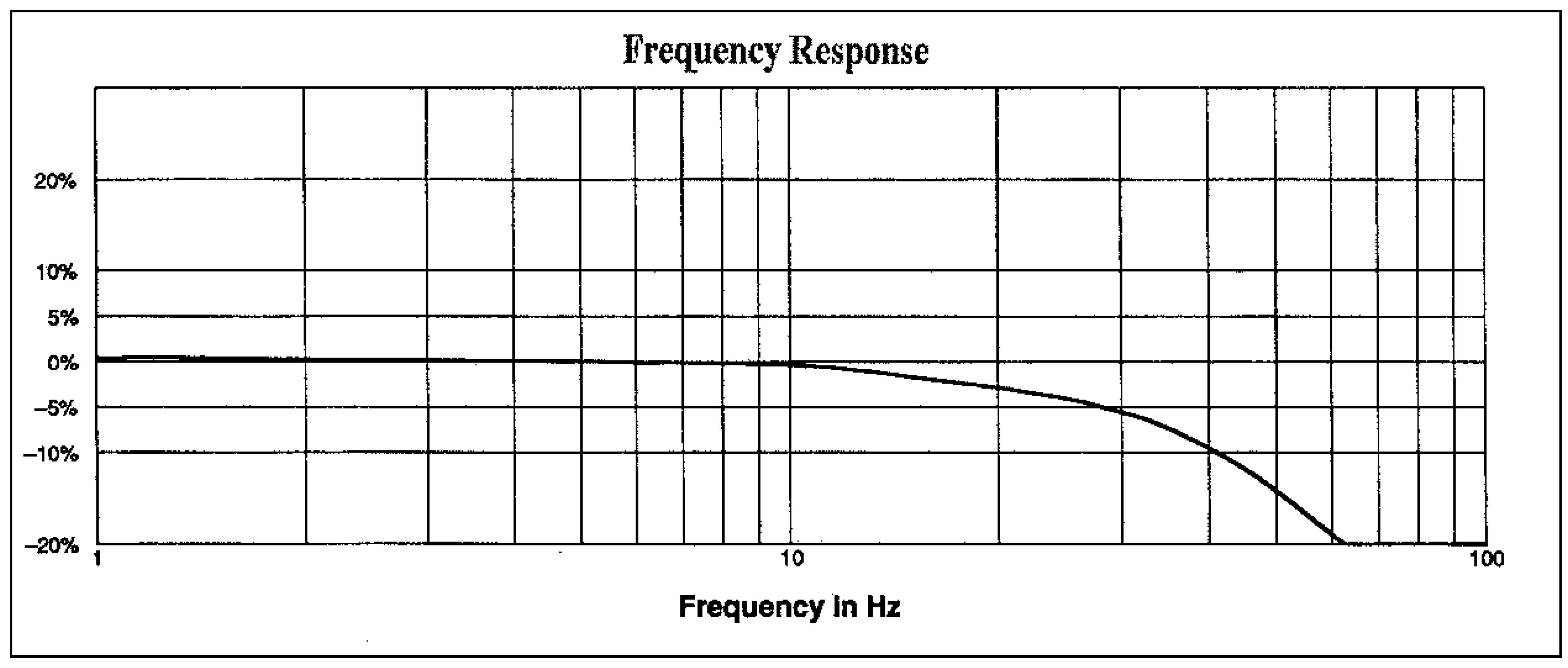
In [1] a reference noise signal was employed as the input to the adaptive filter. This reference signal was derived from a high-pass filter with its –3 dB cut-off frequency at 5 Hz placed at the output of the primary signal. The reference signal (noise source) was taken in such a way that it was uncorrelated with the signal source but correlated with the noise of the primary signal.

In the present paper, a Kalman filter performing as a multivariable optimal filter (in the minimum mean-squares sense) has been implemented to better improve the response of two accelerometers placed on the gravity center of a car under performance tests. These accelerometers were used to measure longitudinal and vertical accelerations. Measurement of these variables, among others, for example: yaw and roll rate, four wheel angular velocities, roll angle, etc., are essential in determining the dynamic behavior of a vehicle and in designing automotive control systems that increase safety and improve handling characteristics.

In this work the Kalman filtering application is an alternative approach that allows us to obtain optimal results and minimize the cost of the instrumentation. In fact, obtaining satisfactory results by other methods (that is, optimal in any other sense) could be more expensive and/or less robust than using this filtering idea.

The outline of contents is as follows:

Section II gives an introduction to the principles of accelerometers and to the wide variety of accelerometers that could be used in different applications. Section III makes some considerations about the use of the classical approach to filtering. Section IV explains the basic Kalman filtering problem. Section V concerns the experimental results, that is to say, the application of the Kalman filter to improve the response of the accelerometers. And Section VI gives the conclusions.

II. Accelerometers

II.1. Accelerometer principles

According to reference [1] and references therein, accelerometers are used to sense vibratory motion, and their measurement method is based on acceleration acting on a spring-mass system in which the movement is normally damped (Figure 1).

Figure 1. Basic spring-mass system: spring, test mass or seismic mass, and damper.

Figure 1. Basic spring-mass system: spring, test mass or seismic mass, and damper.

According to Johnson [10], using Newton’s law and Hook’s law, if the seismic mass, m, is undergoing an acceleration, a, then there must be a force F acting on the mass and given as F₁ = m·a; and the spring of spring constant k is extended (or stretched) from its equilibrium position for a distance Δx, with a force F₂ (opposite to F₁) acting on the spring and given as F₂ = k·Δx.

Thus, under steady-state accelerations, the measurement of acceleration is reduced to a measurement of spring extension (equation 1).

(1)

In analyzing the transient response, we should take into account the friction associated with the seismic mass. Furthermore, if the system exhibits oscillations its frequency of oscillation is calculated as in equation 2, where f_N is the natural frequency (equation 3) and ζ is the dimensionless damping ratio.

(2)

(3)

II.2. Types of accelerometers

There is a wide variety of accelerometers that could be used in different applications depending on the requirements of range, natural frequency, damping, temperature, size, weight, hysteresis, low noise, etc. Piezoelectric Accelerometers, Piezoresistive Accelerometers, Variable Capacitance Accelerometers, LVDT (linear variable differential transformer), Variable Reluctance Accelerometers, Potentiometric Accelerometers, Gyroscopes used for sensing acceleration, Strain Gauges Accelerometers, among others, are a part of the variety of accelerometers.

In these tests two variable capacitance accelerometers were used. The first for sensing longitudinal acceleration, with a range of measurement of ± 2g, sensitivity 985.6mV/g at 5Hz, 1 g pk (g = 9.81m/s²), and transverse sensitivity 0.67%. Figure 2 shows its calibration (temperature 75°F and humidity 57%). And the second for sensing vertical acceleration, with a range of measurement of ± 2g, sensitivity 1002.5mV/g at 5Hz, 1g pk, and transverse sensitivity 0.78%. Figure 3 shows its calibration (temperature 71°F and humidity 48%).

Figure 2. Calibration data (longitudinal accelerometer).

Figure 2. Calibration data (longitudinal accelerometer).

Figure 3. Calibration data (vertical accelerometer).

Figure 3. Calibration data (vertical accelerometer).

III. Some considerations about the use of the classical approach to filtering

According to Anderson and Moore [6], the classical approach to filtering postulates that the useful signals lie in one frequency band and unwanted signals, normally termed noise, lie in another, though on occasions there can be overlap. And when this happens, it is very difficult to eliminate small-magnitude disturbance or interference, and the background noise causes serious difficulties.

In these tests, the frequency bands of the signals of interest and their noise are not strongly mixed with each other; however, the use of low-pass fixed filters with a very sharp cut-off region can introduce problems such as: additional delays, overshoots, and undesirable amplification at some frequency range, etc.

For all the reasons mentioned in this section it is recommended to use optimal signal processing to cancel noise and interference that are usually very hard to cancel using the classical approach to filtering. These reasons, among others, justify the necessity of applying optimal filtering. This is why a Kalman filter is used to diminish the noise in measuring the acceleration of the car under performance tests in this paper.

IV. An introduction to the Kalman filter

According to Anderson and Moore [6], filters were originally seen as circuits or systems with frequency selective behavior. The notion of a filter as a device processing continuous-time signals and possessing frequency selective behavior has been stretched by several developments, and one of the major developments came with the application of statistical ideas to filtering problems. The statistical approaches to filtering postulate that the useful signal and unwanted noise possess certain statistical properties.

The earliest statistical ideas (see ref. [6] and references therein) were related to processes with statistical properties that do not change with time, i.e., stationary processes. However, it was not until the Kalman’s works on optimal filtering [3,4,5] that a theory was developed for coping with nonstationary processes.

IV.1. The filtering problem

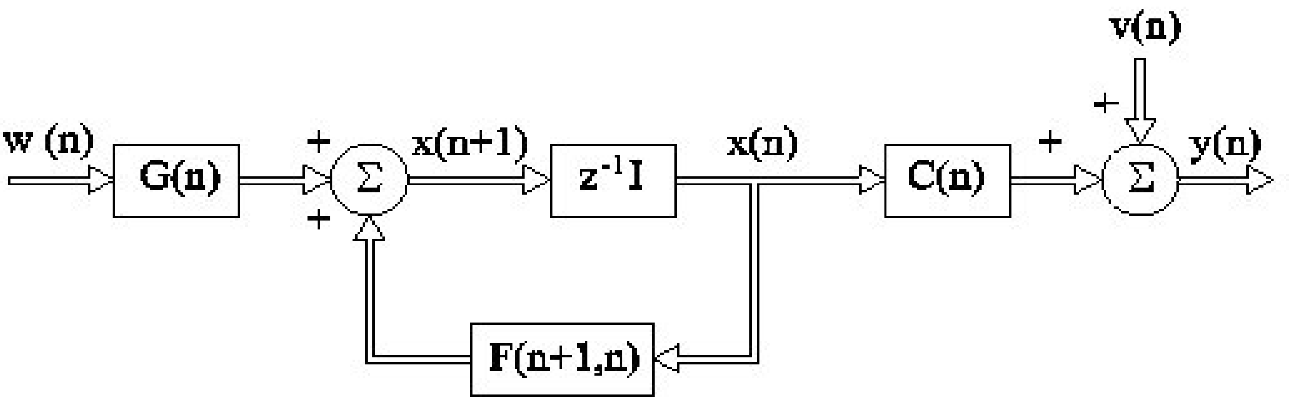
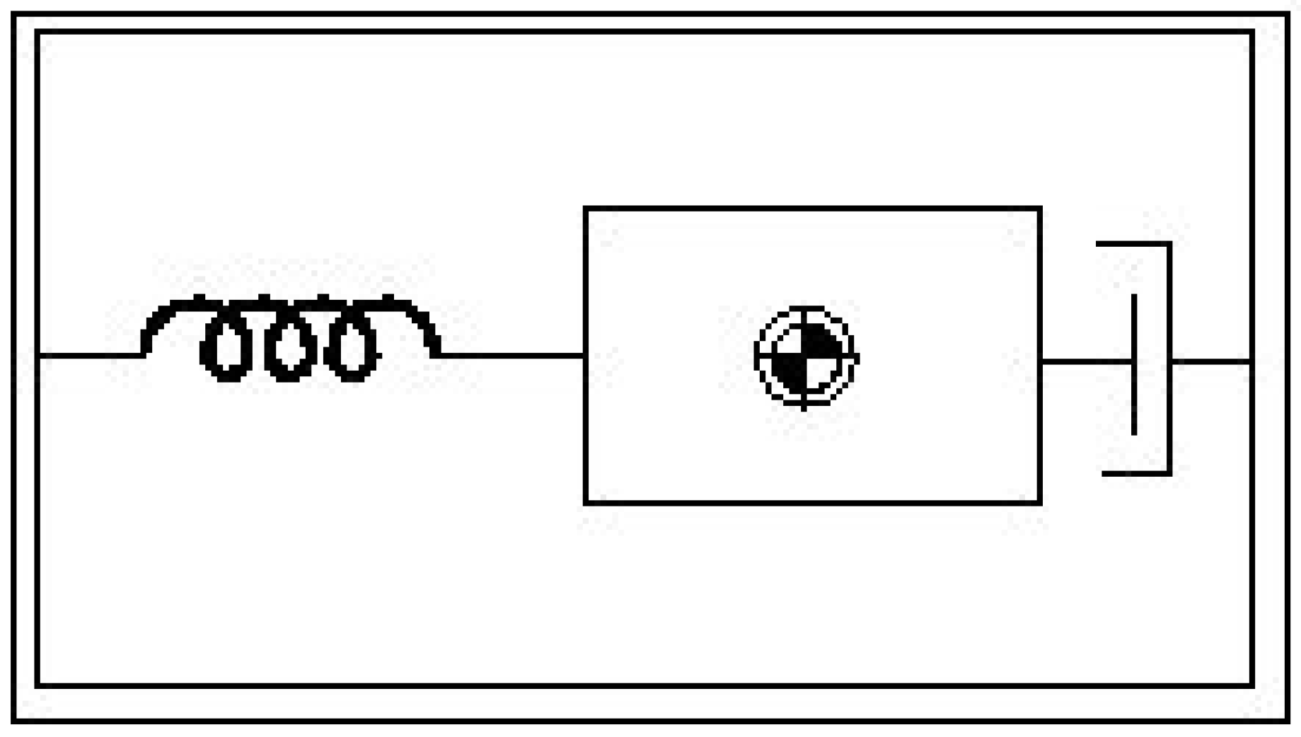
Consider the linear, discrete-time, finite-dimensional dynamical system shown in Figure 4, where I is the identity matrix and z^-1 is the delay. The time-domain description of the system presented here offers important advantages [2], for example:

■

Mathematical and notational convenience

■

Close relationship to physical reality

■

Useful basis for accounting for statistical behavior of the system.

Figure 4. Basic signal model.

Figure 4. Basic signal model.

The system shown in Figure 4 is described by the following state-space equations:

x(n + 1) = F(n + 1,n)x(n) + G(n)w(n)

(4)

y(n) = C(n)x(n) + v(n)

(5)

where equation (4) is the process equation, equation (5) is the measurement equation, n is the time argument (n /0), F(n + 1,n) is a known M-by-M state transition matrix relating the states of the system at times n + 1 and n, G(n) is a M-by-U matrix whose purpose is to color the U-by-1 process noise vector w(n), x(n + 1) is the M-by-1 state vector at time n + 1, x(n) is the M-by-1 state vector at time n, C(n) is a known N-by-M measurement matrix, v(n) is the N-by-1 measurement noise vector, and y(n) is the N-by-1 observation vector. Here, the dimensions of the state vector and the observation vector do not have to be equal to each other. For some cases a relation of N < M is desired, while for others the desired relation between the dimensions of both vectors is N = M. It depends on how many states of the state vector we are interested in estimating.

According to Haykin [2], the vectors w(n) and v(n) are modeled as independent, zero-mean, white-noise vectors (gaussian white process) with covariances given by (6) and (7),

(6)

(7)

where the superscript H denotes Hermitian transposition (i.e., complex conjugation and transposition combined) of a vector or a matrix, Q₁(n) is the correlation matrix of the process noise vector, and Q₂(n) is the correlation matrix of the measurement noise vector. Q₁(n) and Q₂(n) are nonnegative definite for all n.

It is assumed that the initial state x(0) is uncorrelated with w(n) and v(n) for n /0, is a gaussian random variable independent of w(n) and v(n) [2,3,4,5,6,7,8,9]. And the noise vectors w(n) and v(n) are statistically independent processes.

The well known phrase “gaussian white process” is the same as white-noise process, and it comes from the fact that the origins of Kalman filtering lie in the eighteenth century where least squares ideas were used by Gauss in the study of planetary orbits [8,9].

Then the Kalman filtering problem is stated as follows: Use the entire observed data, consisting of the vectors y(1), y(2), ..., y(n), to find for each n /1 the minimum mean-square estimates of the components of the state x(i) [2].

IV.2. Some interpretations

In the previous subsection the Kalman filter property of estimating the state x(n) of the model (4) to (7) was stated. And according to Goodwin and Sin [7], it has the following two interpretations:

If the noise is gaussian, the filter gives the minimum variance estimate of the state; that is, it evaluates the conditional mean of x(n) given the observed data y(1), y(2), ..., y(n).

If the gaussian assumption is removed, the filter gives the linear minimum variance estimate of the state (i.e., having the smallest unconditional error covariance among all linear estimates), but this will not in general be the conditional mean.

IV.3. Summary

Appendix A presents the variables used to formulate the solution to the Kalman filtering problem that have not yet been defined. And a summary of the Kalman filter based on the one-step prediction algorithm is provided in Appendix B.

V. Experimental results: canceling noise in acceleration measurements

In order to get the best information about the complex dynamic of cars and buses, among others, several accelerometers, speedometers, inclinometers, dynamometers, position sensors, etc., should be used and placed in the most important sections of the vehicle under performance tests. This way we are able to take measurements of the vibrations of the framework, chassis, front axle, rear axle, engine, vertical movement, yaw, pitch, roll, and forces and moments on each wheel, etc. However, the instrumentation of a car is sometimes highly expensive and the investment can be reduce since we can get satisfactory measurements using intelligent filtering, prediction and control techniques.

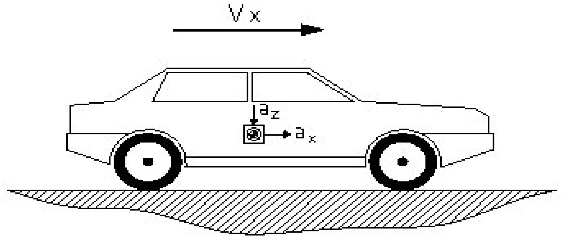
Figure 5 shows the general diagram of the measurement process. The accelerometers were placed on the center of gravity of the car, one to sense longitudinal acceleration (a_x) and the other to sense vertical acceleration (a_z). And a high-precision non-contact speedometer was used to sense longitudinal velocity (v_x), because the contact type of measurement is susceptible to various errors caused by slip, anomalies in the ground surface and unevenness of the road surface.

Figure 5. Representation of the vehicle under performance tests.

Figure 5. Representation of the vehicle under performance tests.

In order to do a satisfactory treatment of the signals under tests, several experiments were done to analyze the power spectral density of these kinds of signals. And, after studying the band-width of these band signals, a sampling frequency of 500 Hz was chosen as a satisfactory sampling rate for the research. Here, the signal processing was done using a personal computer and the National Instruments data adquisition card DAQCard-700.

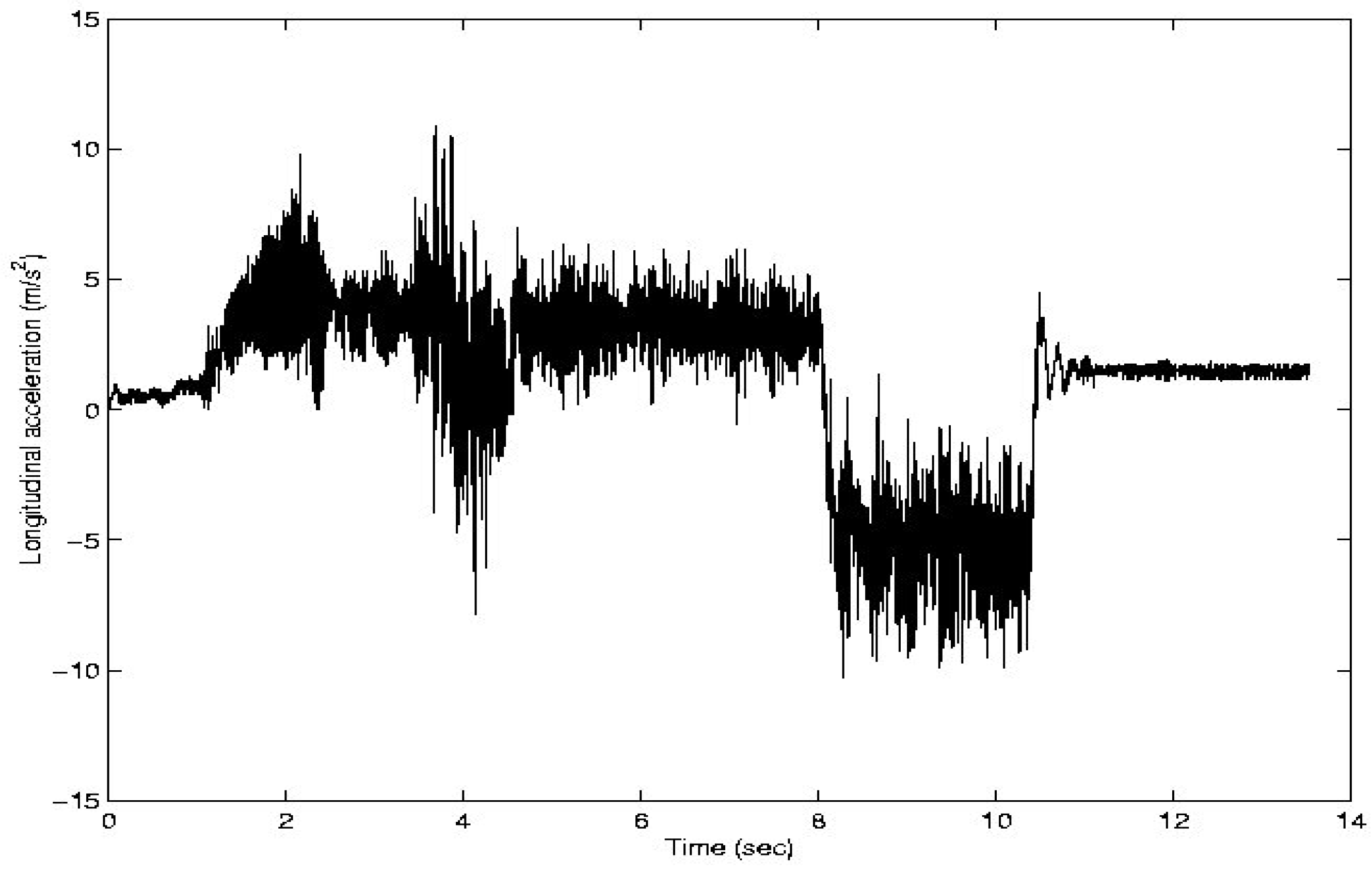
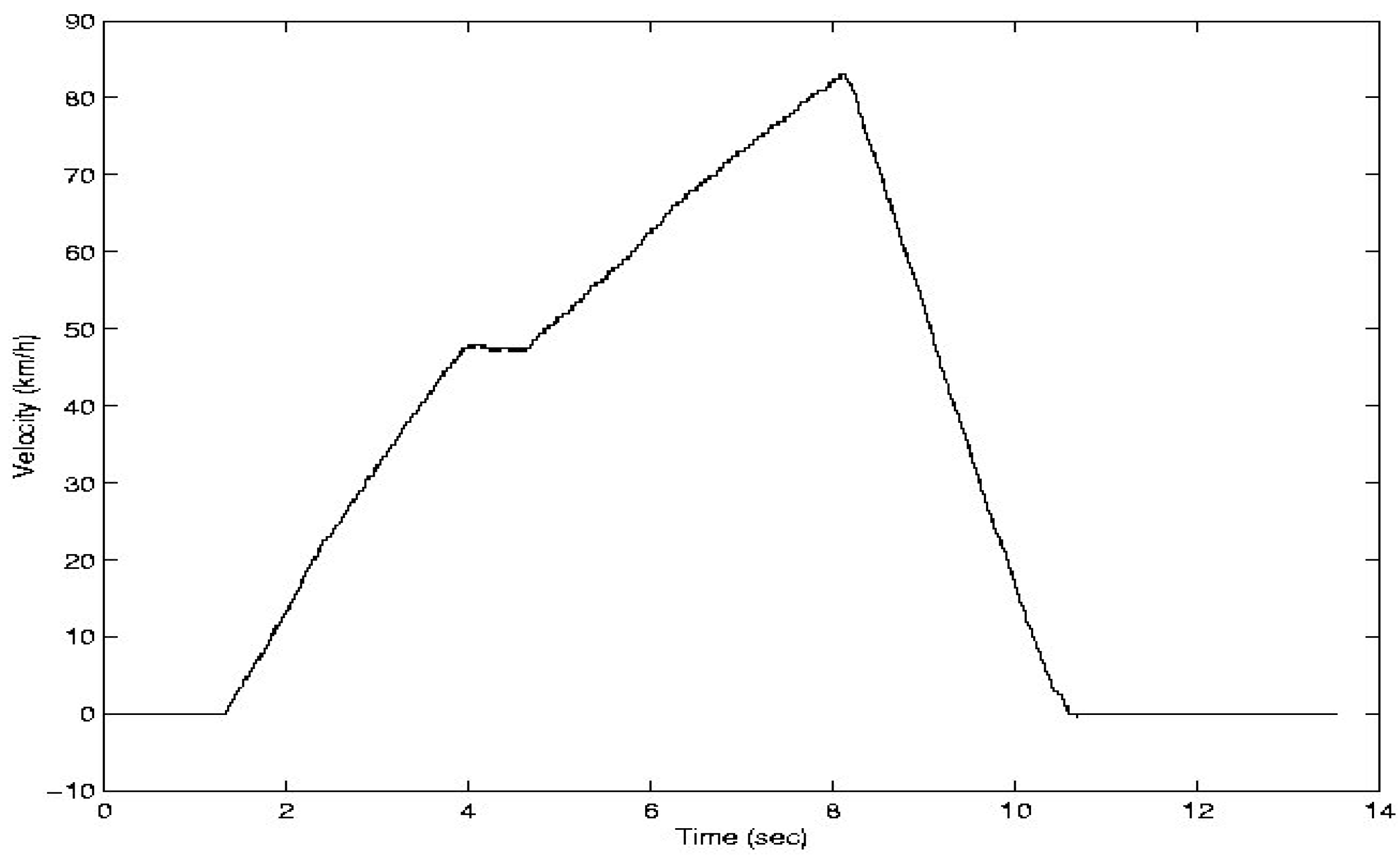
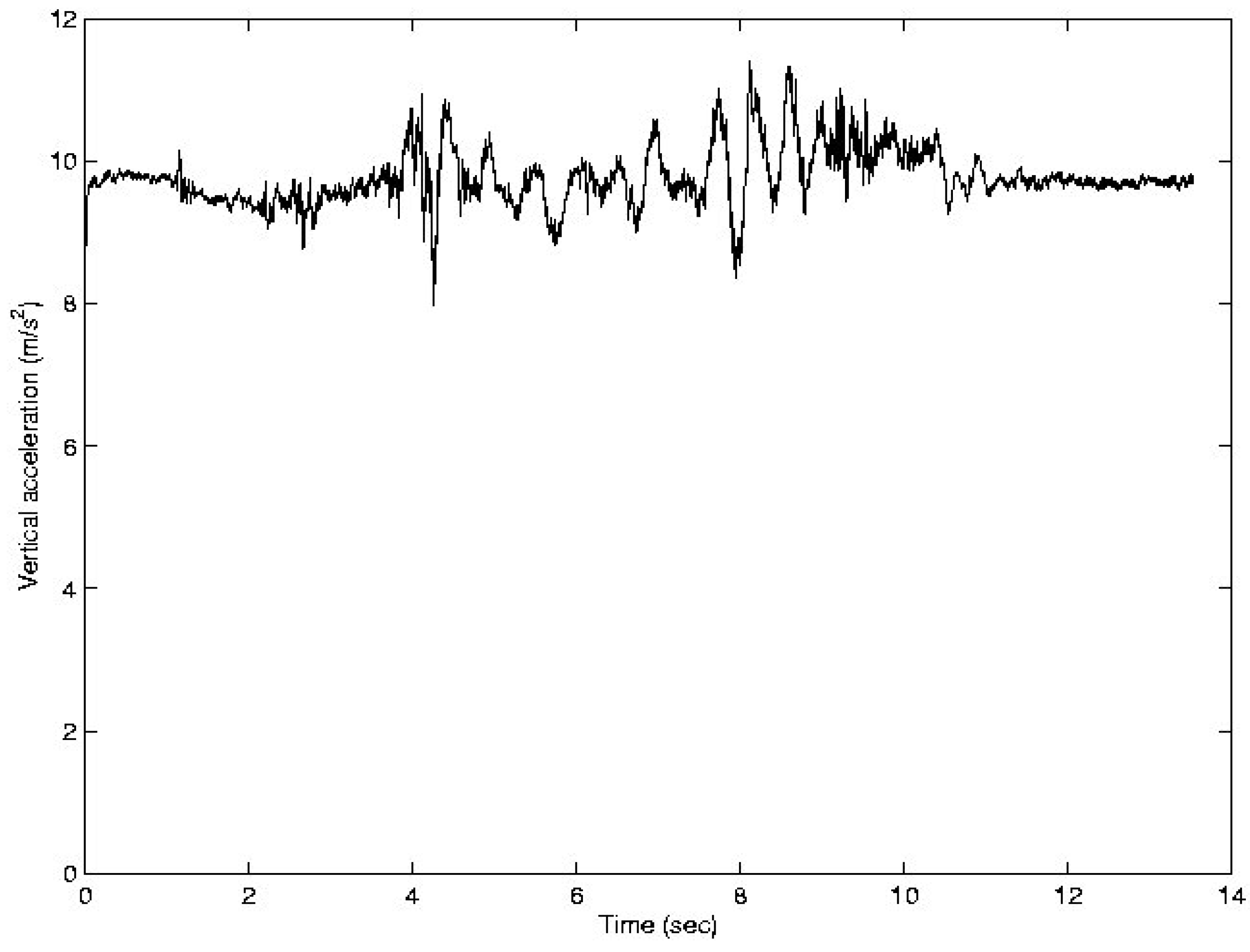
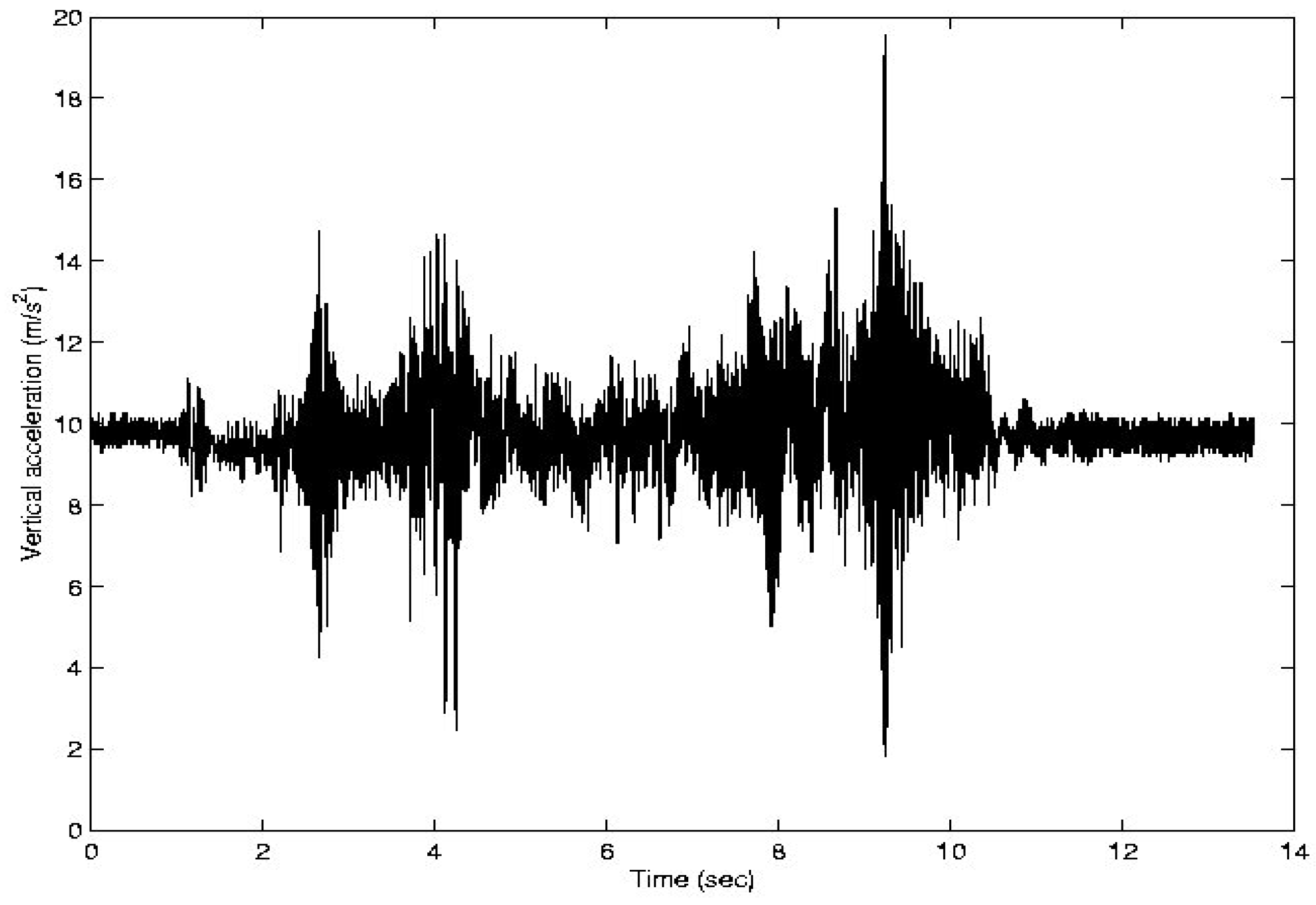
Figure 6 shows the information of the velocity of the car under one of the performance tests, and Figure 7 and Figure 8 show the longitudinal and vertical accelerations, respectively. Note the high level of noise in both signals.

Figure 6. Velocity (km/h) vs. Time (sec).

Figure 6. Velocity (km/h) vs. Time (sec).

Figure 7. Longitudinal acceleration (m/s²) vs. Time (sec).

Figure 7. Longitudinal acceleration (m/s²) vs. Time (sec).

Figure 8. Vertical acceleration (m/s²) vs. Time (sec).

Figure 8. Vertical acceleration (m/s²) vs. Time (sec).

V.1. Necessity of filtering and identifying the main noise sources

As we know, the purpose of filtering is to sort out the information that is desired from something else with which it is contaminated. Here, Figure 7 and Figure 8 show the necessity of filtering these signals corrupted by noise. In this sense, it is important to identify the main noise sources that are affecting the measurements.

So, after a study of vehicle dynamics, suspension systems, and several experiments carried out in the laboratory, it can be said that we have to deal with:

a)

Random signals that have zero mean and fluctuate rapidly in an unpredictable manner, known as white noise;

b)

Colored noise, noise with a bandpass or lowpass spectrum;

c)

Disturbance inputs to the measurement system.

Sensors, electronic circuits and hardware, and the variable road characteristics (treated as a random process in order to reflect real vehicle driving), among others, are sources of white noise and colored noise; and vibrations of the vehicle are sources of colored noise and disturbance.

According to Aparicio et al [2], among others, these vibrations have the following eigenfrecuencies:

1 Hz < eigenfrequency < 3 Hz. Vibrations of the framework and the vehicle sprung masses, vertical movement, yaw, roll and pitch.

4 Hz < eigenfrequency < 8 Hz. Vibrations of the wheels at low speed.

10 Hz < eigenfrecueny < 20 Hz. Vibrations of the vehicle sprung and unsprung masses at medium and high speed, vibrations of the engine, vibrations of the framework, chassis, front axle and rear axle, etc.

These vibrations were taken into consideration as mechanical disturbances affecting the measurement of the accelerometers.

V.2. Implementation and results of the Kalman filter

The state vector x(t) components are longitudinal velocity, and longitudinal and vertical acceleration. The correlation matrix of the process noise vector, Q₁(n), a hypothesis set, used was Q₁ = diag([1e5 1e5]); and the correlation matrix of the measurement noise vector, Q₂(n), a hypothesis set, used was Q₂ = diag([100 100 100]). In both cases, the bigger the components of these matrixes are, the better the response of the filter.

The state-transition matrix, the matrix that colors the process noise vector, and the measurement matrix are shown in equations (8), (9) and (10), respectively. And the initial conditions chosen were and Π₀ = diag([1000 100 100]), where the superscript T denotes vector transposition,

(8)

(9)

(10)

where T_S is the sampling time. Figure 9 and Figure 10 show the estimated values of the longitudinal and vertical acceleration, respectively. The results show that Kalman filtering provides good estimates of the vehicle variables under tests. The method presented here gives state estimates that can be used for advanced feedback control and help us to create the basis to make intelligent driving decisions. The Kalman filter performs as an Infinite Impulse Response filter and provides the best prediction in the minimum mean-square sense of the signals of interest.

Figure 9. Estimated value of the longitudinal acceleration.

Figure 9. Estimated value of the longitudinal acceleration.

Figure 10. Estimated value of the vertical acceleration.

Figure 10. Estimated value of the vertical acceleration.

V.2.1. Signal-to-noise ratio improvement

For the purpose of this subsection equation (5) is rewritten as in (11). Then, the measurements y(n) comprise signal z(n) and noise v(n), with signal power E[z(n)²] and noise power E[v(n)²]. So, the filter input signal-to-noise ratio (SNR) is defined by (12).

y(n) = z(n) + v(n) = C(n)x(n) + v(n)

(11)

(12)

In order to calculate the filter output SNR, it has to be taken into consideration that the output of the true filter is , from which . And, by the orthogonality principle, is orthogonal to . Then, equation (13) defines the total filter output power, and the filter output SNR is defined by (14).

(13)

(14)

The results of the application of the equations (12) and (14) are that:

1)

For the longitudinal acceleration, the Filter input SNR is approximately –17.9 dB and the Filter output SNR is approximately 17 dB;

2)

For the vertical acceleration, the Filter input SNR is approximately –1.6 dB and the Filter output SNR is approximately 39 dB.

VI. Conclusions

In this paper a Kalman filter was used to diminish the noise in measuring corrupted signals. This research focused on the acceleration of a car under performance tests. Both measurements of acceleration were taken by using low-cost accelerometers, and signal-to-noise ratio improvements higher than 30 dB were achieved, which is a good performance factor for judging the quality of the filter. The experimental results contribute to enrich the importance of bridging the gap between optimal sensing and optimal signal conditioning.