In Situ Ecophysiology of Microbial Biofilm Communities Analyzed by CMEIAS Computer-Assisted Microscopy at  Single-Cell Resolution

Dazzo, Frank B.; Klemmer, Kevin J.; Chandler, Ryan; Yanni, Youssef G.

doi:10.3390/d5030426

Open AccessArticle

In Situ Ecophysiology of Microbial Biofilm Communities Analyzed by CMEIAS Computer-Assisted Microscopy at Single-Cell Resolution

by

Frank B. Dazzo

^1,*,

Kevin J. Klemmer

¹,

Ryan Chandler

¹ and

Youssef G. Yanni

²

¹

Department of Microbiology and Molecular Genetics, Michigan State University, East Lansing, MI 48824, USA

²

Department of Soil Microbiology, Sakha Agricultural Research Station, Kafr El-Sheikh 33137, Egypt

^*

Author to whom correspondence should be addressed.

Diversity 2013, 5(3), 426-460; https://doi.org/10.3390/d5030426

Submission received: 22 April 2013 / Revised: 15 May 2013 / Accepted: 27 May 2013 / Published: 25 June 2013

(This article belongs to the Special Issue Microbial Ecology and Diversity)

Download

Browse Figures

Versions Notes

Abstract

:

This paper describes the utility of CMEIAS (Center for Microbial Ecology Image Analysis System) computer-assisted microscopy to extract data from accurately segmented images that provide 63 different insights into the ecophysiology of microbial populations and communities within biofilms and other habitats. Topics include quantitative assessments of: (i) morphological diversity as an indicator of impacts that substratum physicochemistries have on biofilm community structure and dominance-rarity relationships among populations; (ii) morphotype-specific distributions of biovolume body size that relate microbial allometric scaling, metabolic activity and growth physiology; (iii) fractal geometry of optimal cellular positioning for efficient utilization of allocated nutrient resources; (iv) morphotype-specific stress responses to starvation, environmental disturbance and bacteriovory predation; (v) patterns of spatial distribution indicating positive and negative cell–cell interactions affecting their colonization behavior; and (vi) significant methodological improvements to increase the accuracy of color-discriminated ecophysiology, e.g., differentiation of cell viability based on cell membrane integrity, cellular respiratory activity, phylogenetically differentiated substrate utilization, and N-acyl homoserine lactone-mediated cell–cell communication by bacteria while colonizing plant roots. The intensity of these ecophysiological attributes commonly varies at the individual cell level, emphasizing the importance of analyzing them at single-cell resolution and the proper spatial scale at which they occur in situ.

Keywords:

allometric scaling; biofilm; biogeography; CMEIAS image analysis; community analysis; computer-assisted microscopy; microbial ecophysiology; morphological diversity; single-cell microbiology; spatial ecology

Graphical Abstract

1. Introduction

A major challenge in microbial ecology is to develop reliable methods of computer-assisted microscopy that can analyze complex digital images of microorganisms at single cell resolution and reveal insights about their ecology in situ without cultivation. To address this challenge, our team of microbiologists, mathematicians and computer scientists has been developing software applications that can accurately process digital images of actively growing microbial populations and communities in natural and managed habitats, and extract an abundance of ecologically relevant data from them. The long-range goal is to develop and release a comprehensive suite of software applications designed to strengthen quantitative, microscopy-based approaches for understanding microbial ecology at spatial scales relevant to the individual microbes and their ecological niches. Our software suite is called CMEIAS (Center for Microbial Ecology Image Analysis System), and as components become fully developed and documented, they are released for free download at our project website [1]. The CMEIAS ver. 3.10 currently being developed [2] is a significant upgrade of the earlier released version 1.27 [3], and inter alia, includes an ecophysiology module based on motivation to create quantitative computing tools that can help users obtain better, statistically defendable answers to pertinent questions on physiological attributes of microbial populations and communities during their biofilm colonization of biological and non-biological surfaces.

A long-term goal of this approach is to integrate multiple methods of ecological statistics performed on CMEIAS acquired data into coherent and consistent models and take full advantage of their predictive power. This paper documents the use of computer-assisted microscopy to extract the wealth of ecologically relevant information present in accurately segmented images of microbial populations and communities, and various quantitative methods to analyze those attributes to reveal insights about microbial ecophysiology in situ. The intensity of these attributes commonly varies at the individual cell level, emphasizing the importance of analyzing them at single-cell resolution and the proper spatial scale at which they occur.

2. Experimental Section

Submerging transparent microscope slides in aquatic environments [4] provides a simple approach to produce natural assemblages of microbial biofilm communities suitable for detailed morphological analysis using computer-assisted microscopy. The microbial assemblages described here were developed on clean microscope slides of plain borosilicate glass or polystyrene plastic polymer (Erie Scientific, Portsmouth New Hampshire) submerged for four summer days from a fishing line 1 foot below the surface of the Red Cedar River that flows through the campus of Michigan State University (East Lansing, MI, USA). Slides were retrieved and their underside wiped clean. The slides were mounted in filter-sterilized water with a No. 1.5 thickness glass cover slip, oiled above and below the slide, and examined by phase-contrast light microscopy using a 100 × Planapochromat Phase 3 objective lens to resolve individual bacterial cells. Digital 8-bit grayscale images of the biofilms were acquired using a monochrome digital camera, then segmented to binary, combined into composite images, spatially calibrated and analyzed using CMEIAS image analysis software [2,3] to produce the 2-dimensional coordinate systems that accurately define the location and morphology of individual attached bacterial cells at 0.2 μm spatial resolution. Extracted data were analyzed statistically using StatistiXL [5], EcoStat [6], Ecological Methodology [7], PAST [8], Species Diversity and Richness [9], GS + Geostatistics [10], and an in-house CMEIAS Data ToolPack software application [2].

Methods to acquire digital micrographs and segment the foreground objects for in situ studies of bacterial viability, metabolic respiration, cell–cell communication, and phylogenetically differentiated substrate utilization are described elsewhere [11,12,13,14].

3. Results and Discussion

3.1. Images of Microbial Community Biofilms and Their Spatial Abundance

Figure 1 shows accurately segmented digital images that represent the mixed populations of microbes in immature biofilms that developed in situ on plain glass (a) and polystyrene plastic (b) substrata submerged in a freshwater aquatic ecosystem. These two representative microbial assemblages, named biofilm communities “A” and “B”, have different diversities, growth physiologies, metabolic activities and biogeographies reflecting the strong influence that substratum physicochemistry exerts on development of freshwater aquatic microbial biofilm communities before they become confluent.

Table 1 reports the spatial intensity of the microbes in these two biofilm assemblages, each standardized to landscapes of equal substratum surface areas. The substratum area captured in each image was 10,360 um², the biovolume formula was shape-adapted with assumed axial symmetry, and their biomass carbon was calculated using the allometric conversion of 200 fg C/um³ of cell biovolume [2,15]. The results indicate an increased abundance and intensity of colonization by the microbial biofilm community B on the polystyrene substratum in the freshwater aquatic ecosystem. These data set the stage for exploring the measurement attributes that CMEIAS can extract from these images to gain insight into the ecophysiological forces that structure these differences in microbial community ecology, thereby shedding light on ways that the environmental variable of hydrophobicity (associated with polystyrene) in substratum physicochemistry impacts on development and cell–cell interactions of sessile microbial communities and biofilm architecture in freshwater aquatic ecosystems.

Figure 1. Binary images of natural microbial biofilm assemblages (communities A and B) developing on (a) plain glass slides and (b) polystyrene plastic slides submerged for four summer days in the Red Cedar River, East Lansing Michigan. Bar scales equal 10 μm.

Table 1. Spatial intensity in microbial community A and B freshwater biofilms developed for four days on plain glass and polystyrene substrata (Figure 1a,b), respectively.

**Table 1.** Spatial intensity in microbial community A and B freshwater biofilms developed for four days on plain glass and polystyrene substrata (Figure 1a,b), respectively.
Spatial Abundance Parameter	Community A	Community B
Spatial Density (cells/mm²)	155,790	159,554
Microbial Coverage of the Substratum (%)	7.0	10.8
Cell Length Intensity (um/mm²)	154,568	215,049
Biosurface Area Intensity (um²/mm²)	272,798	398,226
Biovolume Intensity (um³/mm²)	34,513	68,799
Biomass Carbon Intensity (pg C/mm²)	6,903	13,760

3.2. Biofilm Diversity and Ecophysiology Indicated by Morphological Analyses of the Biofilm Communities

3.2.1. Background

Diversity embraces the concept of heterogeneity in community structure, and incorporates information on the richness and distribution of abundance among population classes [16]. The diversity of a microbial assemblage is inherently important to understand its structure and function at all levels of biological organization. Ecological theory (based primarily on studies of plants and animals) predicts that basic differences in biology between species, including niche requirements and tropic level, inevitably generate substantial differences in abundance among species [16]. Thus, the distributions of species abundance can shed light on the processes that determine the biological diversity of the assemblage.

Several approaches are available to quantify community diversity, each emphasizing a particular set of characteristics that impact on the ecophysiological potential and functional redundancy of each population contained within it. Common methods of microbial diversity analysis include classification schemes applied to growth responses of organisms in various differential culture media [17], profiling of phospholipid-derived fatty acid biomarkers [18,19], nutritional versatility [20], and a variety of 16S rRNA gene-based techniques [21,22]. The latter approach is currently the most commonly used to assess microbial diversity, with its strength anchored in the large, ever-expanding and freely available online searchable databases of indexed sequences and supporting tools of computational bioinformatics (e.g., [23]), and the relatively low cost to obtain the phylogenetically relevant nucleotide sequences nowadays. These approaches can be complemented with computer-assisted microscopy and image analysis of morphological diversity, where each individual cell in accurately segmented images is digitally analyzed in silico using multidimensional pattern recognition algorithms and then classified within milliseconds to the appropriate morphotype to ≥0.01% rarity [2,3]. The unique, supervised, hierarchical morphotype classifier featured in CMEIAS operates within 14-dimensional space using mathematical rules of pattern recognition algorithms that are fully tested and documented, performs with an overall accuracy of ~96%, and has user-defined features to accommodate the ~4% error rate [3]. The resultant information on morphotaxa-based richness and distribution of abundance can contribute to the powerful complementary approach of polyphasic taxonomy (especially when combined with 16S rDNA-based methods) for microbial community analysis, reflecting the diversity of niche apportionments in the community being studied [3,16,17,18,19,20,21,22,23,24,25]. Also, inclusion of morphology-based analyses in a polyphasic-based approach can shed additional light on in situ ecophysiological assessments of community membership-environment relationships, allometric scaling indicative of their metabolic rate and biomass productivity, nutrient resource allocation and utilization efficiency when competing for limiting resources, indices of community health, integrity and functional stability affecting community resilience, dominance-rarity relationships reflecting environmental stability and ecological succession, and various morphologically-expressed adaptations following stress-induced perturbations (starvation, predation, eutrophication, etc.) in the same community [3,16,24,25,26,27,28,29,30,31,32].

3.2.2. Effect of Substratum Chemistry on Biofilm Community Structure

Figure 2a,b is the CMEIAS-rendered images of the same two biofilm community assemblages (Figure 1a,b) showing each microbe distinctively pseudocolored according to its assigned morphotype classification. These pseudocolored images are automatically produced as an output of the software classification routine. Readily apparent in both communities are the numerically dominant cocci (red) and regular rods (blue), and the numerically less abundant prosthecates (yellow), unbranched filaments (aqua), curved rods (purple), and ellipsoids (true green). In addition, detailed inspection of the images reveals the rare occurrence of U-shaped rod (pink) and club (olive green) morphotypes that are uniquely present only in the biofilm assemblage of community B (Figure 2b).

The relative abundance of morphotype-specific classes (Table 2) in communities can be evaluated in discrete units (individual cell counts) or in continuous scale (biovolume body size), each reflecting their niche apportionment in communities and how they change following environmental perturbation or natural succession [16]. The small apportionment of the richness among very abundant morphotypes (2/6 and 2/8 for Communities A and B, respectively) compared to the large apportionment of “rare” morphotypes (<25% relative abundance) commonly occurs when only one or a few factors dominate the ecology of the assemblage [16]. Diversity levels may be higher when other methods are included in the polyphasic taxonomy approach. The alpha diversity statistics (Table 3) describe the heterogeneity in biofilm community membership at spatially defined units [26]. The indices of diversity, dominance, and evenness are computed from the data on the richness in number of different morphotype classes in the two assemblages and the variations in distribution of abundance among each of them [6,7,8,9,16,26].

When abundance is scored by either metric (individual cell counts and cell biovolume), the evenness in distribution of morphotype classes is higher (hence, lower dominance) for the biofilm assemblage colonized on the polystyrene surface (community B), and thus that hydrophobic substratum favors developed of a microbial biofilm community with greater diversity than the community A developed on plain glass (Table 2, Table 3). The Simpson diversity index (1/D) is highest among the group of diversity indices tested because it is heavily weighted towards the most abundant class. Evenness indices are typically higher when abundance is biovolume-weighted (Table 3) since its discrimination of morphotype sizes commonly shows that few larger morphotypes will compensate for the smaller, more numerically abundant morphotypes. The Simpson Dominance and Berger-Parker Dominance indices, which indicate the proportional importance in community membership of the most abundant classes, are larger when abundance is measured as individual counts rather than biovolume. The Solow statistical randomization test of significance using a 10,000-iterated partition [9,33] indicated that the computed differences in these indices between community pairs are statistically significant at the 5% level (Table 3). Thus, the diversity of morphotype populations in the community can be described as having a pyramid-shaped structure (many small and few large individuals) that is less steep when abundance is scored by their biovolume body mass.

Figure 2. CMEIAS-rendered pseudocolor images indicating the morphotype classification for each individual microbe in situ within biofilm assemblages of communities A (a) and B (b) See text for details.

Table 2. The distribution of abundance for each morphotype class in images of biofilm communities A and B.

**Table 2.** The distribution of abundance for each morphotype class in images of biofilm communities A and B.
MorphotypeClass	Individual Cell Counts		Cumulative Cell Biovolumes (μm³)
MorphotypeClass	Community A	Community B	Community A	Community B
Coccus	1262	1122	157.24	185.84
Regular Rod	312	450	118.44	128.56
Unbranched Filament	6	29	28.35	261.57
Prosthecate	20	23	9.01	7.86
Ellipsoid	2	22	0.76	38.31
Curved Rod	12	3	5.14	1.98
U-Shaped Rod	0	2	0	1.17
Club	0	2	0	1.59
Morphotype Richness	6	8	6	8

Table 3. Indices of diversity, evenness, dominance and dissimilarity for communities A and B. Statistically significant (p < 0.05) higher values are indicated with superscript ^a in the comparison of communities A vs. B when using the same morphotype abundance metric (e.g., community A vs. B using cell counts), and are indicated with the superscript ^b in the comparison of counts vs. biovolume as the abundance metric for the same community (e.g., comparing cell counts vs. biovolume for Community A).

**Table 3.** Indices of diversity, evenness, dominance and dissimilarity for communities A and B. Statistically significant (p < 0.05) higher values are indicated with superscript ^a in the comparison of communities A vs. B when using the same morphotype abundance metric (e.g., community A vs. B using cell counts), and are indicated with the superscript ^b in the comparison of counts vs. biovolume as the abundance metric for the same community (e.g., comparing cell counts vs. biovolume for Community A).
Diversity Index Metric	Index Computed from Differentiated Cell Counts		Index Computed from Differentiated Cell Biovolumes
Diversity Index Metric	Community A	Community B	Community A	Community B
Simpson Diversity (1/D)	1.541	1.868^a	2.575 ^b	3.260 ^a^,b
Shannon-Weiner H’ Diversity	0.630	0.833^a	1.115^b	1.322^a^,b
Brillouin D Diversity	0.623	0.824^a	1.082^b	1.299 ^a^,b
Shannon-Pielou J Evenness	0.303	0.401^a	0.536^b	0.636^a^,b
Simpson Dominance	0.646 ^a^,b	0.535^b	0.384 ^a	0.307
Berger-Parker Dominance	0.782 ^a^,b	0.679^b	0.494 ^a	0.417
% Dissimilarity	10.88		39.19

These differences in community structure are also reflected in the Renyi diversity ordering and Whittaker ranked abundance plots shown in Figure 3a,b, respectively. The Renyi ordering analysis shows the relative magnitude of diversity changes when several different indices are used [9]. Its plot (Figure 3a) indicates that the greater relative diversity in community B is robust for multiple diversity indices when the metric of abundance is either individual counts or biovolume body mass, and the computed diversity is always higher using biovolume body size rather than individual cell counts as the abundance metric for both communities. The shape of the Whittaker rank/abundance curve indicates the dominance and evenness of the community [16]. The plotted data (Figure 3b) has a shallower declining slope when biovolume is the metric of abundance, indicating higher evenness in distribution of abundance between morphotype classes in these biofilm assemblages.

These distinctions are important because the relative abundance of populations within a community to some extent reflects their success at competing for limited resources [16], and therefore the metric used to measure abundance in community membership can significantly influence how variations in that relationship are interpreted. This point extends to all methods to measure abundance in community analysis. The β diversity index of percent dissimilarity indicates that the ability to distinguish community diversity is 3- to 4-fold higher when using the metric of morphotype-specific biovolume rather than individual counts per morphotype class. Consideration of these results allows one to appreciate the significant discriminating power that morphotype classification combined with biovolume measurements provides when analyzing microbial communities in situ.

Ecological theory predicts important interrelationships between the relative proportions of dominant to rare members in a community and the stability of the environment in which they have colonized [16,28]. The presence of rare species is predicted to indicate a successional process in which later colonists have requirements that are more specific and hence are rarer [16,34]. Polyphasic taxonomy analyses of methanogenic anaerobic bioreactor communities show that the driving force responsible for high resilience following environmental perturbation is the flexibility in responsiveness of the significantly important rare members of the microbial community rather than the magnitude of community diversity as a whole [3,24,25]. Interestingly, analysis of microbial communities in agricultural soils have indicated that soil bacteria captured by standard bacteriological culturing methods are either represented in very low abundance or not detected when the same community membership is analyzed by the culture-independent sequence analysis of amplified 16S rDNA [35]. Considered collectively, the important implication of these findings is that “rarity” among class membership in microbial communities is “conditional” [35] and does not necessarily imply unimportance since they can represent viable components actively occupying ecological niches in the community and can make significant contributions to its stability and resilience following environmental perturbation [24,25].

Figure 3. Renyi ordering (a) and Whittaker (b) ranked abundance plots that compare the diversity of morphotype classes in communities A and B when individual cell counts and biovolume body size are used as the metric of class abundance.

These theoretical principles provide the framework for a quantitative analysis focused on dominance-rarity relationships in community structure performed on data acquired by computer-assisted microscopy. One method uses a K-dominance analysis to examine the contribution of each morphotype class by plotting its percentage cumulative abundance against log class rank in the community [16,28]. Communities differ in diversity when their K-dominance curves do not overlap. Less diverse assemblages dominated by only a few (morpho)taxa will accumulate percentage abundance with more elevated curves than will more diverse assemblages [8,28]. This is the case for the biofilm assemblage of community A, indicating that its greater intensity of dominance (Figure 4a) contributes to its lower diversity (Table 2). A second method in dominance-rarity analysis produces a 2-dimensional Gaston Quartile Rarity scatterplot [16,29], where the quartiles in the two distributions are shown by dotted lines (Figure 4b). Morphotype classes are considered rare when located in the first (lower left) quartile (25th percentile) of the scatterplot [29]. Note that the majority of morphotype richness for both communities A and B is represented by classes that fit the criteria of rarity (Table 2, Table 3, Figure 4a,b). Ecological theory would predict that they have experienced ecological succession in the aquatic ecosystem [16,29].

Figure 4. (a) K-Dominance and (b) Quartile Rarity scatter plots that compare the extent of dominant and rare morphotype classes within the communities. Dotted lines in 4b indicate the 25th percentile for both axes that define the first quartile of rare morphotype classes.

3.2.3. Morphotype-Influenced Allometry, Nutrient Allocation, Reproductive Strategy and Starvation Survival

The abundance of a species to some extent reflects its success in competing for limiting resources. In addition to the insights provided by biovolume as a measure of abundance (as described above), this metric can also be used to explore distributions of individual body size, which is the hallmark of allometric scaling. This ecophysiological characteristic addresses the relationships between metabolic rate and body size, which governs many observed patterns in ecology. Allometric scaling relates body size proportional to nutrient resource concentration and allocation in an environment and the consequential metabolic performance and growth rate of the organisms in the community [26,30]. Body size determines resource use, how the fractal nature of food cluster availability and concentration trade‐off with body size, and how species body size constrains its ability to coexist with other species [16,26]. Multiple species can coexist on the same limited resource and occupy the same or very similar niche space within the community because they differ in body size, diet, and resource demand [16,26].

Pertinent to the importance of allometric scaling in microbial ecophysiology is their sizing down as an adaptation to the starvation-imposed stress of nutrient limitations in an environment [31,32]. As nutrients become scarcer and the cell enters a state of starvation survival (e.g., stringent response triggered by amino acid deprivation), its body size is decreased by reductive division accompanied by an increase in surface area to volume ratio that enhances its efficiency to capture more nutrients for utilization and provide better distribution of those resources once inside the cell. These ecophysiological changes in body size are accompanied by various phenotypic changes including increased efficiency of nutrient uptake systems, increased production of flagella and pili, remodeling of their cell envelope architecture, turnover of ribosomes and utilization of internal storage polymers to satisfy their maintenance energy requirements for survival in the absence of growth. Optimal cell size depends negatively on the size of resource molecules when resource uptake is limited by diffusive transport and membrane uptake [27]. When competing for two resources of different molecular sizes, two different-sized consumers can coexist if the inputs of resources and sizes of consumers are correctly chosen [27]. Thus, individual body size can provide a first, best surrogate approximation of its habitat-specific concentration, allocation and acquisition of nutrient resources, metabolic rate and growth physiology [16]. This information can provide insights to distinguish autochthonous (oligotrophic) k reproductive strategists whose small body size and increased ratio of surface area/volume allow them to grow slowly while successfully adapting to starvation stress, and outcompete zymogenous (copiotrophic) r reproductive strategists when nutrient concentrations are very low. In contrast, the zymogenous r strategists are limited by their carrying capacity and grow faster, allowing them to outcompete others when external concentrations of essential nutrients are high.

The 99.3% higher abundance of total microbial biovolume per unit of substratum area in the biofilm assemblage of community B (Table 1) provided the first clue suggesting differences in allometric scaling of microbes in these two communities. Those results were corroborated with differences in spatial abundance of biomass carbon and biosurface area (Table 1). To test this hypothesis further, various statistical analyses were performed on the arrays of cell biovolume data extracted from each microbe in the biofilm images of communities A and B (Figure 1a,b and Table 4). The Shapiro-Wilks test rejected the null hypothesis of normality (p < 0.0001), indicating that neither array of individual cell biovolumes was normally distributed. The median metric of central tendency for the distribution of biovolume sizes was larger for all cells in community B, and the 2-tailed non-parametric Mann-Whitney test indicated that this difference was statistically highly significant. This result prompted us to identify which morphotype class(es) contribute(s) most to distinguish this allometric scaling relationship. The Shapiro-Wilks test of individual cell biovolumes for each separate morphotype class indicated normal distributions for the ellipsoids, curved rods and prosthecates, and non-normal distributions for the cocci, regular rods and unbranched filaments. We therefore used the mean and median, respectively, as the metrics of central tendency in the parametric and non-parametric tests of differences between the distributions of individual cell biovolumes for each morphotype class in the two communities.

The results of these tests varied depending on the morphotype examined. The distribution of individual cell biovolumes of the cocci and ellipsoid morphotypes contributed most to ranking the higher allometric scaling relationships in community B. The small probability of those results being due to chance was 5.1 × 10⁻⁸ and 4.0 × 10⁻⁵, respectively. Although the median cell biovolume was higher for regular rods in community A, that difference was not sufficient to raise the rank of allometric scaling to be statistically higher than that found in community B. In addition, the Student t and Mann-Whitney test statistics indicated that the distributions of cell biovolumes for the curved rod, prosthecate and unbranched filament morphotypes in both communities were not significantly different. The difference in body size for the unbranched filaments is visually apparent but quantitatively insufficient to reject the null hypothesis of equal medians.

The corollary of these results was further evaluated by comparing the surface area/volume ratios for all cells in the two communities and their distributions among different morphotype classes (Table 4). The anticipated results occurred, with significantly higher values of the surface area/volume indicator of cellular starvation stress in community A evaluated in whole (Table 4). The major contributors to this overall result were the significantly higher values for the cocci and ellipsoid morphotypes in community A. The surface area/volume values were not significantly different for the curved rod, prosthecate and unbranched filament morphotypes. Interestingly, regular rods had higher values for this metric in community B, but again, that result was not statistically sufficient to raise the rank of starvation stress above that found in community A.

Table 4. Tests for normality and differences between mean or median of individual cell biovolumes and surface area/biovolume ratio for microbial morphotype classes in communities A and B. The superscript ^a denotes higher values (Community A vs. Community B) that are statistically significant at the indicated p level, based on the appropriate 2-tailed Student t (for mean) or Mann-Whitney (for median) inference tests.

**Table 4.** Tests for normality and differences between mean or median of individual cell biovolumes and surface area/biovolume ratio for microbial morphotype classes in communities A and B. The superscript ^a denotes higher values (Community A vs. Community B) that are statistically significant at the indicated p level, based on the appropriate 2-tailed Student t (for mean) or Mann-Whitney (for median) inference tests.
Component Analyzed	Normality?; Median or Mean of Cell Biovolume (μm³); p value	Normality?; Median or Mean of Cell Surface Area/Volume (μm⁻¹); p value
Whole Biofilm Community A	No; Median = 0.077	No; Median = 12.665^a;
Whole Biofilm Community A	No; Median = 0.077	p = 1.22 × 10⁻¹⁴
Whole Biofilm Community B	No; Median = 0.143^a; p = 1.1 × 10⁻¹²	No; Median = 10.827
Coccus-Community A	No; Median = 0.052	No; Median = 14.763^a;
Coccus-Community A	No; Median = 0.052	p = 2.09 × 10⁻¹⁴
Coccus-Community B	No; Median = 0.084^a; p = 5.05 × 10⁻⁸	No; Median = 11.362
Ellipsoid-Community A	Yes; Mean = 0.391	No; Median = 6.441^a; p = 0.01
Ellipsoid-Community B	Yes; Mean = 1.784^a; p = 4.0 × 10⁻⁵	No; Median = 3.740
Curved Rod-Community A	Yes; Mean = 0.463;	Yes; Mean = 9.634; p = 0.436
Curved Rod-Community B	Yes; Mean = 0.489; p = 0.804	Yes; Mean = 9.111
Prosthecate-Community A	Yes; Mean = 0.450; p = 0.138	No; Median = 13.679
Prosthecate-Community B	Yes; Mean = 0.347	No; Median = 14.655; p = 0.535
Unbranched Filament-Community A	No; Median = 2.554; p = 0.948	No; Median = 10.487; p = 0.584
Unbranched Filament-Community B	No; Median = 1.337	No; Median = 9.301
Regular Rod-Community A	No; Median = 0.275^a; p = 7.30 × 10⁻¹⁰	No; Median = 9.209
Regular Rod-Community B	No; Median = 0.225	No; Median = 10.387^a; p = 0.001

These results illustrate how the ability of CMEIAS to discriminate microbial morphotypes can help to evaluate allometric scaling and nutrient allocation relationships within microbial communities. Morphotype-specific differences in intensity for these indicators all point to the impact that the hydrophobic polystyrene substratum imposes on the growth ecophysiology of microbial biofilm communities in the freshwater aquatic ecosystem. Considered collectively, the statistical results provide strong evidence that cocci and ellipsoid morphotypes of community B developing on the polystyrene substratum have access to a higher level of nutrient resources that promote higher metabolic and growth rates, larger body sizes, and a zymogenous k-type reproductive strategy. In contrast, members of community A developing on the plain glass substratum exhibit evidence of significant nutrient limitation and reduced metabolic/growth rate that triggered their adaptations to starvation stress, including reduction in body size concurrent with increase in surface area/volume ratio that would enhance their nutrient uptake efficiencies to perform with an autochthonous r-type reproductive strategy under the prevailing conditions. Predictably, nutrients concentrate higher on the polystyrene substratum, allowing selected microbial morphotypes in the biofilm community B to sustain higher metabolic activity and growth on its surface.

Allometric scaling can also provide insight into the intensity at which communities respond to environmental change. In this case, cumulative percentages of abundance measured by cell counts and body mass are plotted against a log scale of ranked classes to produce Abundance/Biomass Comparison (ABC) curves. These ABC plots (derived from K-dominance concepts) are useful to explore if assemblage diversity is affected by an environmental perturbation at the landscape location, and if so, the cumulative effect of that disturbance [16,36]. Both plots (Figure 5a,b) showed elevated curves of cumulative percent abundance measured by cell counts. This type of relationship is common when the local environment has perturbed the community structure that it supports, resulting in ecological succession [16]. The degree of separation between the curves for counts vs. biovolume is slightly greater for the biofilm community B developed on the hydrophobic polystyrene substratum, suggesting that its response to environmental perturbation was slightly more intense.

Figure 5. Abundance/biomass comparison (ABC) plots for community assemblage A (a) and B (b). Greater separation of the two curves implicates a more intense ecophysiological response of the community to environmental change or perturbation.

3.2.4. Morphological Indicators of Predatory Stress Affecting Microbial Community Structure

Predation is not evenly distributed across organism size classes. Instead, size‐selective and morphology‐selective predation behaviors can structure the abundance and diversity of community membership. Body size significantly influences the natural diversity‐modifying, community‐structuring effects of predator‐selective rather than random foraging behavior, in line with the evolutionary pressure to maximize their resource intake [26]. Bacteriovory grazing activies by heterotrophic protozoan nanoflagellates and metazoan predators are important forces that shapen the structure and composition of bacterial communities in aquatic ecosystems, largely because resistance to and refuge from selective bacteriovory is favored by large cell aggregates and elongated filamentous morphologies that exceed the oral diameter (equivalent to gape-size) of the cytosome or lorica mouth opening, thereby increasing the difficulty of engulfing and consuming them by the predators [37,38]. Thus, the relative abundance of filamentous microbes can be used to indicate the intensity of the selective pressure of phagotrophic predatory stress that contributes to shaping the aquatic microbial community. Visual inspection of the microbial assemblage images (Figure 1a,b) and the CMEIAS-rendered, pseudocolored morphotype classification images (Figure 2a,b) indicates a significantly higher abundance of unbranched filaments in biofilm community B. This was confirmed by image analysis, indicating that community B has a 4.7-fold higher abundance of that morphotype (Table 2), and indeed, its biovolume body mass dominates all morphotype classes in that assemblage (41.7% of total). These results predict that bacteriovory grazing activities were more intense in the biofilm assemblage of community B, and the increased fittness of the elongated unbranched filament morphotype amidst the selective predatory stress has resulted in its dominance.

3.2.5. Biofilm Ecophysiology of Nutrient Acquisition and Utilization Efficiency Indicated by its Landscape Fractal Dimension

At the core of the allometric scaling relationships in ecophysiology are the local variations in nutrient resource allocation. Acquiring enough food is the first key requirement for successful colonization of surfaces by microbes. Various ecological studies suggest that metabolic processes used for growth physiology rely on the hierarchical fractal-like nature of resource distribution networks, and that organisms have exploited a fourth spatial dimension by evolving hierarchical fractal-like structured spatial distributions designed to maximize nutrient resource acquisition, allocation and efficiency [39]. Fractal descriptions of this self-similarity metric for communities provide quantitative insights about the spatial distribution of resources in situ and how organisms compete for and exploit those resources [26]. This fractal partitioning of heterogeneous distributions and allocations of the same resource is an important trade‐off constraint that enables the coexistence of multiple species among community members [26]. Thus, a landscape analysis of fractal geometry can provide insights that help to explain the ecophysiology of microbial colonization behavior on surfaces, driven by their food cluster availability, nutrient resource allocation and optimal positioning to maximize their utilization efficiency.

Microbial biofilms exhibit self-similar fractal geometry at multiple spatial scales [40,41], reflecting the complexity of their architecture and microcolony coastline borders. The ability to discriminate fractal dimensions along coastlines of microcolony biofilm patches and the spatial patterns of microbes at single-cell resolution within biofilms is being implemented in a new CMEIAS software application, currently at its near final stage of development [2,42]. Image analysis of the spatial positioning of individual microbes in the two biofilm assemblages (Figure 1a,b) indicate that both landscapes exhibit positive fractal geometry (Table 5). The higher fractal dimension of the community B assemblage is consistent with the enhanced complexity of its landscape structure, suggesting that the spatially aggregated cells in that biofilm are more effectively positioned to optimize their efficient utilization of nutrient resources provided in the flowing aquatic habitat of the Red Cedar River. This higher intensity of fractal-like positioning of cells in community B (Table 5) and their higher metabolic rate predicted by their allometric scaling (Table 4) support the model that this natural biofilm assemblage has more effectively dispersed to and colonized microenvironments on the slides where local nutrients have concentrated at distances relevant to their niche, thus contributing to their overall higher spatial structure, productivity and diversity on the hydrophobic polystyrene substratum.

Table 5. Fractal geometry of the natural biofilm assemblages of microbial communities A and B developing on plain glass and polystyrene substrata, respectively. The higher values of fractal dimension are indicated by upward arrows.

**Table 5.** Fractal geometry of the natural biofilm assemblages of microbial communities A and B developing on plain glass and polystyrene substrata, respectively. The higher values of fractal dimension are indicated by upward arrows.
Fractal Dimension Method	Community A Biofilm	Community B Biofilm
Dilation	1.20196	1.30069 ↑
Euclidean Distance Map	1.15666	1.25709 ↑
Box Counting	1.03285	1.23618 ↑
Cumulative Intersection	1.53651	1.75074 ↑

3.3. Biofilm Ecophysiology Indicated by Spatial Pattern Analysis

3.3.1. Background

Spatial patterns of distribution among community members influence many processes that are ecologically important [43]. Because many ecological processes are scale-dependent, their study should include a spatial component measured at the scale in which the process occurs [43]. A major goal of spatial analysis in ecophysiological studies is to define what a measured characteristic at one location can reveal about that same characteristic at neighboring locations. Analyses of in situ spatial ecology are designed to scrutinize distribution patterns at a given spatial scale and produce predictive ecological models of colonization behavior that help to reveal the ecophysiological processes occurring in that habitat [43].

The quantification of spatial heterogeneity is necessary to elucidate relationships between ecological processes and spatial patterns [43]. The essence of the statistical pattern analysis is to distinguish between spatial distributions of the organisms that can be explained by random chance versus those that cannot. The benchmark of that assessment tests the null hypothesis that the patterns have complete spatial randomness represented by a Poisson distribution with means equal to variance. Complete spatial randomness implies that no microbial interactions affect the events resulting in their spatial pattern of colonization. In contrast, statistically significant deviations from complete randomness in spatial patterns can reflect phenotypic ecophysiological adaptations in spatially structured landscapes, indicating that localized and/or regionalized microbial interactions have affected their colonization behavior resulting in the spatial pattern present.

Non-random spatial structures may not only result from ecological interactions; they may also play an essential functional role in organizing the interactions that dictate their ecophysiology and stability [44]. Spatial patterns of microbial colonization that are aggregated (clustered) imply positive (cooperative and/or mutualistic) interactions among neighboring cells that have promoted each other’s growth ecophysiology. Extreme examples of this relationship occur in interspecies coaggregates of cross-feeding, e.g., syntrophic microbial species residing in methanogenic communities. Aggregated patterns of distribution in landscape structures also result from the scale-dependent heterogeneous fractal variability in limiting resource partitioning, and reflect the high efficiency at which cells actively disperse and cooperatively position themselves spatially and physiologically when faced with the interactive forces of microbial coexistence to optimize their allocation of nutrient resources on a local competitive scale [26]. In contrast, patterns of spatial uniformity (regularity) imply negative (inhibitory and/or antagonistic) interactions that have resulted in their maximally separated, over-dispersed, self-avoiding colonization behavior. This information is of significant ecophysiological importance because spatial heterogeneity resulting from both types of nonrandom patterns between individuals (aggregated or uniform) tends to stabilize ecological systems [44,45] and can explain much of the species diversity that coexists in a community colonizing a habitat [26]. Key issues in spatial pattern analysis that typically follow statistical rejection of the null hypothesis of complete spatial randomness include whether the pattern exhibits uniform regularity or coaggregation, the spatial scale at which the pattern of interaction is defined (local vs. regional), and the statistical strength of that pattern’s departure from randomness [45].

Does location really matter in microbial ecophysiology? Do the patterns of microbial spatial distribution represent “ecological music” or are they no more than random noise? The common answer is yes indeed, location does matter and structured patterns of microbial spatial distribution can be magnificently symphonic. Spatial segregation of morphotypes colonizing the same habitat can provide insights into their feeding behavior, trophic level, food web dynamics and reproductive capacity. This trend has consistently been found in our spatial ecology studies of microbial biofilms that develop in a variety of natural and managed habitats, including plant rhizoplanes and phylloplanes [46,47,48,49], freshwater streambed pebbles [50], and microscope slides suspended in various river/lake ecosystems [2,51,52].

Microbial colonization of local areas low in nutrient availability leads to poor productivity with a tendency to form overdispersed spatial patterns indicative of intense competition, whereas colonization of nutritionally enriched microenvironments results in increased growth that flourishes as aggregated patterns of local microcolony biofilms [51,52]. Central to these negative (conflicting) and positive (cooperative) interactions are various molecular cell–cell communication events that regulate the ecophysiology affecting microbial colonization behavior and biofilm architecture [52]. Also, knowing the location and intensity of clustered behavior for microorganisms can improve the understanding of the underlying processes that generate and sustain the interdependent microbe-environment relationships within biofilm architectures and the spatial scale at which they occur [51,52]. Thus, modeling spatial patterns of microbial communities at multiple spatial scales is crucial to understand their ecophysiological functioning fully. Indeed, no study of microbial ecophysiology is complete without an in situ spatial consideration of their activities within the habitat, simply because everything is not randomly located everywhere. Applying spatial statistics to analyze microbial biofilm architectures can also provide insight on the ecological forces that underlie the basic mechanisms of the colonization behavior that created them.

3.3.2. Point Pattern Spatial Distribution Analysis

CMEIAS is designed to analyze three different categories of microbial spatial distribution. The first category is a plot-less “point pattern,” based on extraction of the in situ micrometer scaled distances between each bacterial cell and its nearest neighbor within the biofilm landscape. Spatial attributes included in these analyses are the X|Y Cartesian coordinates of each cell’s centroid position (relative to the assigned 0, 0 landmark position located at the lower left corner of the image), the μm scaled distance from each object’s centroid to its first and second nearest bacterial neighbors, and the empirical distribution function of first nearest neighbor distances.

Several analyses of spatial point patterns were performed on the two biofilm communities for this study. The first involved a calculation of the Clark and Evan’s Randomness Index intended to test for departure from complete spatial randomness in the overall landscape structure. This spatial statistic is computed from data of the first nearest neighbor distances between cells and the spatial density within the biofilm landscape. The mean neighboring distances were greater for observed than expected values, Z values were greater than the threshold border of 1.96, and R indices were greater than 1.00 (Table 6). These results detect statistically significant departure of complete spatial randomness for spatial patterns in both biofilm assemblages, including uniform patterns signalling negative over-dispersed conflicts of self-avoiding colonization behavior that are more intense in biofilms of Community A than in Community B (p values of 3.21 × 10⁻⁶⁴ and 2.78 × 10⁻⁵, respectively).

Table 6. Clark and Evans spatial point pattern test for complete spatial randomness of cells in biofilm communities A and B. Calculations are based on landscape areas defined by the convex hull of point distributions with Donnelly edge correction [8].

**Table 6.** Clark and Evans spatial point pattern test for complete spatial randomness of cells in biofilm communities A and B. Calculations are based on landscape areas defined by the convex hull of point distributions with Donnelly edge correction [8].
Point Pattern Statistic	Community A	Community B
Observed Mean Distance	1.5125	1.3191
Expected Mean Distance	1.2331	1.2494
Z test statistic	16.92	4.2168
R Index	1.266	1.056

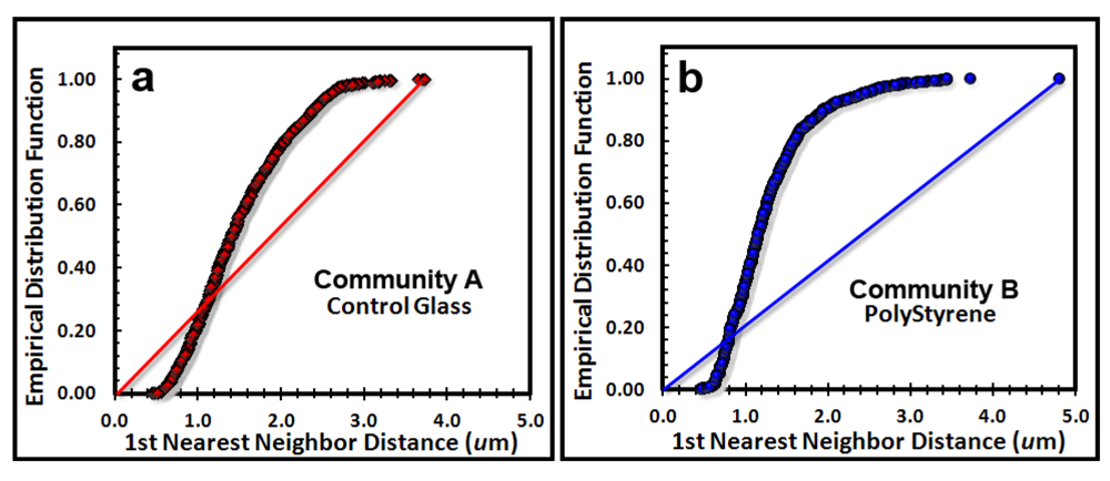
The next point pattern analysis evaluated the Empirical Distribution Function (EDF) of the cells’ spatial distribution, which produces a plot that compares the cumulative ranking of the first nearest neighbor distances between individual cells in the sample to the theoretical distribution that would result if the pattern were completely random (indicated by a diagonal random trendline that extends from the XY intercept to the maximum nearest neighbor distance found in the analysis). Datapoints indicate a uniform pattern of distribution when they form a tight group with little range of first neighbor distance, an aggregated distribution when the curve ascends to form a distinct extended asymptote at EDF of 1.00 above the random diagonal trendline, and a random distribution when the EDF curve ascend with a shallower slope closer to the diagonal trendline. Differences in intensity of aggregated patterns are indicated by their relative distance above the diagonal trendline of complete spatial randomness. The empirical distribution plot for the biofilm landscapes (Figure 6a,b) indicate a greater portion of uniformly dispersed pattern for Community A (consistent with Clark and Evans R index, Table 6), and a steeper curve displaced further above the blue diagonal trendline for Community B, indicating that Community B has a more intense aggregated pattern than does Community A, whose EDF curve is shallower and closer to the red diagonal trendline.

Ripley’s K [53] multi-distance spatial cluster analysis is a useful sequel to the EDF analysis. This is a second-order, point distribution statistic that evaluates the co-occurrence of separation distances between pairs of object points to determine if the point pattern changes with distance of the spatial scale of analysis. The K(d) function measures the average count of objects enclosed within circles of radius d that are centered on every object point in the landscape divided by the mean spatial density of objects in that landscape. A plot of all K(d) functions vs. all radial separation distances for all objects in the landscape indicates if the pattern is uniformly dispersed, clustered or enclosed within a Monte Carlo simulation of the confidence envelope representing the 95% critical limits for a test of complete spatial randomness. Observed K(d) values represent uniform spatial distributions when located below the confidence envelope of spatial randomness, and represent clustered distributions when located above the confidence envelope. The intensity of clustering or uniformity is indicated by the relative proportion and location of observed points whose separation distances lie above or below the statistically defined 95% envelope of spatial randomness, respectively.

Figure 6. Cumulative empirical distribution function of the first nearest neighbor distances between individual bacteria within biofilm assemblages of community A (a) and community B (b). The diagonal trendline of complete spatial randomness is indicated in both plots for comparison.

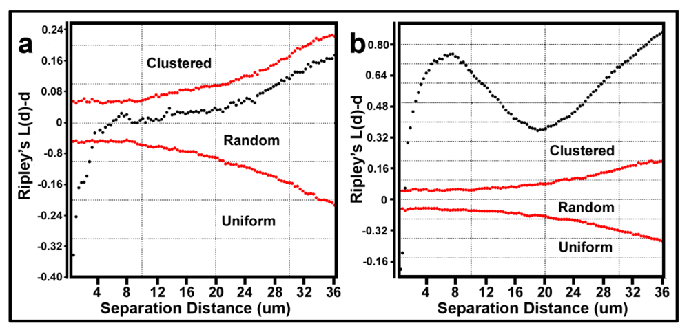
The Donnelly edge-corrected [7,8] and standardized Ripley K (L(d)-d) [8] values of point pattern characteristics for all bacteria within biofilm community assemblages developing on the plain glass and polystyrene substrata are plotted in Figure 7a,b respectively. Several features of these two Ripley K plots reveal statistically significant information that dramatically distinguishes the spatial patterns of the microbes at different spatial scales in these two biofilm assemblages. First, some cells in both biofilm landscapes are uniformly equidistant from each other. These occur at eight different separation distances in community A and two different separation distances in community B. Second, the majority of separation distances is represented by cells with random spatial distribution in community A, and by cells that are spatially aggregated in community B (note the larger Y-axis scale in Figure 7b). Third, the distribution of K functions for spatially aggregated cells in Community B has a discrete mode of local interactions at separation distances of approximately 6–8 μm (up to 18 μm) and another mode of regional interactions at a maximum of 36 μm. These interesting results indicate that the biofilm landscape that developed on the polystyrene substratum is significantly more spatially aggregated than the biofilm developed on plain glass. This distinction of colonization behavior revealed by the Ripley K analysis illustrates how the spatial structure of second-order interactions within microbial biofilms can be significantly influenced by the (physico)chemistry of the substratum upon which it develops.

Figure 7. Donnelly edge-corrected and standardized Ripley K plots of point pattern characteristics for all bacteria within biofilm community assemblages of communities A and B developing on the (a) plain glass and (b) polystyrene substrata. The results indicate that most cells are randomly distributed in Community A and clustered in Community B.

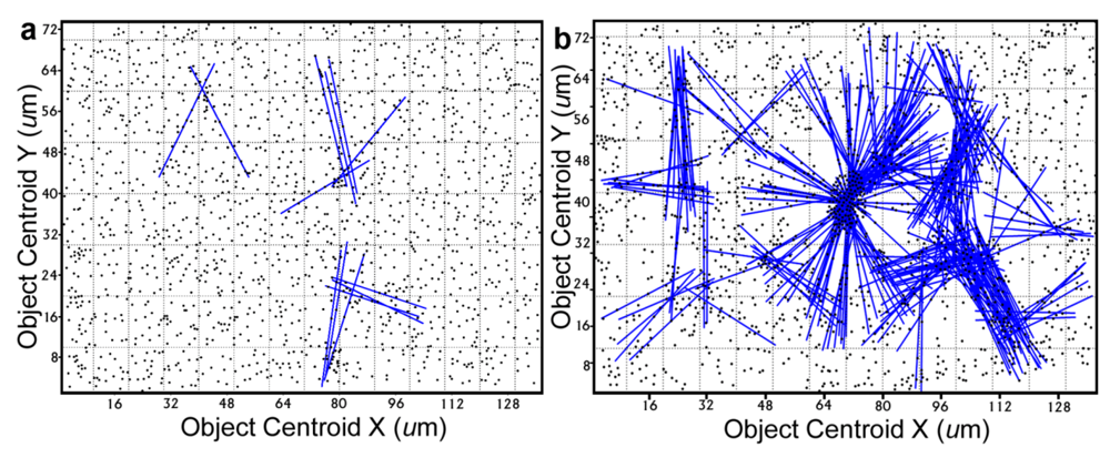
Further definition of the location, intensity and radial dimension of bacterial interactions emanating from discrete spatial aggregates within biofilms can be predicted from 2-dimensional plots of their line segment patterns. These plots indicate the statistically significant linear point alignments (Figure 8a,b) whose angular orientations dramatically illustrate the directionality of multiple intersecting “hot spot” epicenters of interpoint interactions [8,54] that are strongest within clusters of closely neighboring bacteria in the biofilm communities. As anticipated, the numbers of linear point alignments and clustered “hot-spot” epicenters of positive interpoint interactions between closely aggregated bacteria are significantly greater in the biofilm community B, and they point in all compass directions (Table 7).

Figure 8. Line segment pattern plots of statistically significant linear point alignments whose intersecting angular orientations locate numerous “hot-spot” epicenters of clustered bacterial interactions within the biofilms communities A (a) and B (b).

Table 7. Intensity of the line segment patterns indicating clustered bacterial interactions in Figure 8a,b.

**Table 7.** Intensity of the line segment patterns indicating clustered bacterial interactions in Figure 8a,b.
Biofilm Landscape	Point Alignment Lines	Point Alignment Epicenters
Community A	13	4
Community B	242	31

3.3.3. Quadrat-Lattice Spatial Distribution Analysis

The second category of pattern analysis performed on spatial data is called a plot-based or gridded “quadrat-lattice” analysis of dispersion, based on the frequencies of individual object counts within equal-sized quadrats from the corresponding images. Evaluation of both biofilm landscape images using the CMEIAS Quadrat Maker tool [2] indicated that a 7 × 7 grid of 49 square quadrats was optimal for this analysis (figure not shown). The spatial pattern analysis of the gridded data indicated that cells in community A had a mix of random to slightly aggregated distribution, and cells in biofilm community B exhibited a significant greater intensity of aggregated pattern of distribution (Table 8).

Table 8. Plot-based quadrat-lattice spatial pattern analysis of biofilm communities A and B.

**Table 8.** Plot-based quadrat-lattice spatial pattern analysis of biofilm communities A and B.
Quadrat Spatial Pattern Index	Biofilm Landscape	Value	P value & Interpretation
Variance : Mean Ratio	Community A	1.226	(p = 0.136); random pattern
Variance : Mean Ratio	Community B	8.454	(p = 0.001), Significantly aggregated
Morista Standardized Dispersion Index	Community A	0.258	Slightly aggregated
Morista Standardized Dispersion Index	Community B	0.502	Significantly aggregated

3.3.4. Geostatistical Spatial Distribution Analysis

The third category of spatial pattern analysis performed on spatial data is called a geostatistical analysis. This robust method of analysis measures the degree of dependency among observations in a geographic space to evaluate the continuity or continuous variation of spatial patterns over that entire spatial domain [55]. Geostatistics tests whether a user-defined, continuously distributed variable is spatial autocorrelated, i.e., exhibits spatial structure. The result of the analysis quantifies the spatial uncertainty about the high irregularity of regionalized variables and the scale of their spatial correlation. It indicates whether the events among pairs of cells at one location influence that same measured variable associated with their cell neighbors at more distant locations. Patterns displaying spatial autocorrelation indicate that operations of colonization behavior involve a spatially explicit process rather than occur randomly and independent of their location. It quantifies the resemblance of the measured parameter between neighbors as a function of their separation distance. Geospatial data are autocorrelated when close neighbors are more similar (as in aggregated distributions) than are neighbors locate further apart [56]. When found, the autocorrelation can be accurately modeled using its weighted average from neighboring sampled locations to connect various spatially dependent relationships derived from regionalized variable theory, plus make optimal, statistically rigorous interpolation (kriging) maps of the parameter at unmeasured locations within that spatial domain.

Geostatistical analysis and krig mapping require that the relevant parameter being analyzed (the so-called “Z variate”) is a quantitative (non-binary) metric that is continuously distributed over the spatial domain, and that the sampling sites are georeferenced at known X, Y Cartesian coordinates relative to a landmark position in the same landscape (commonly set to 0, 0 coordinates at the lower left corner of the image) [10,55]. We developed the CMEIAS cluster index as the major Z-variate to conduct geostatistical analyses of bacterial surface colonization behavior at single-cell resolution [57]. CMEIAS computes this cluster index as the inverse of the separation distance between the object centroid of each bacterial cell and its first nearest cell neighbor. This index is an example of a local indicator of spatial association whose magnitude reflects the intensity of each cell’s clustered distribution in relation to other cells in its local environment. Used as such, it performs well as a sensitive sensor of positive, spatially autocorrelated cell-to-cell interactions that cooperatively promote bacterial colonization behavior in situ [51,52,57]. Cells with a high cluster index are typically arranged in aggregated patterns that facilitate cell communications, resulting in positive metabolic cooperations that promote their localized growth into populations of microcolony biofilms [47,51,52,57,58].

The heterogeneity in cluster index assigned to cells within the landscape domain of the biofilm can be evaluated several ways. One method is to produce a 3-dimensional georeferenced bubble scatterplot where each cell in the biofilm landscape is represented by a bubble whose diameter (width) is weighted by its individual CMEIAS cluster index. The information provided by this spatial aggregation analysis reveals the significant variable of spatial proximity among individual cells in the biofilm over the entire landscape domain, which is more important than a quorum of high population density per se in governing the success of cell–cell communication within biofilms [12]. First, an object analysis is performed on the spatially calibrated image to extract the XYZ data from every cell, indicating its X,Y Cartesian posting locations relative to the landmark origin and the Z coordinate of its cluster index. These georeferenced data are then used to produce the 3-dimensional bubble scatterplot, indicating the X, Y spatial position of every cell and the magnitude of its associated cluster index. This analysis shows the proximity and intensity of spatial coaggregation where positive cell–cell interactions affecting colonization behavior are likely to occur. 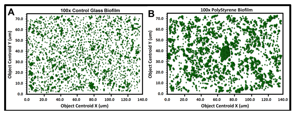Figure 9a,b show the bubble plots for all cells in the biofilm assemblages of communities A and B, respectively. The significantly larger and more numerous clustered bubbles in the biofilm landscape of community B clearly indicate higher spatial aggregation of cells, with implication that its spatial heterogeneity would define the intensity of diffusion gradients of chemical signals and other bioactive metabolites that influence their biofilm ecophysiological activities, including colonization behavior.

The second type of geostatistical analysis is designed to produce the variogram plot, which defines the extent that the measured Z-variate for each cell exhibits spatial dependence between pairs of sample locations. This plot relates the uncertainty of regionalized variables with the distances that they autocorrelate. It statistically describes how autocorrelated values at two points begin to become different as the separation distance between them increases. That information provides the profoundly important and statistically defendable estimate of the real micrometer range of spatial scale of separation distances at which individual neighboring cells can influence each other’s Z-variate.

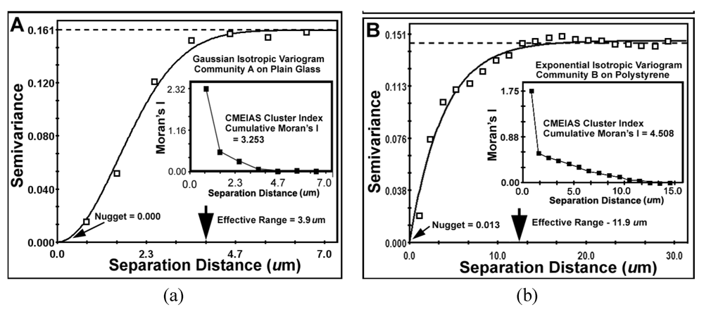
The results of key metrics derived from the geostatistical autocorrelation analysis are presented in Table 9 and Figure 10a,b. The computed mathematical models of the geostatistical data for both communities made a statistically highly significant fit (r²) indicating that the cluster index Z-variate is spatial autocorrelated. These best-fit models are isotropic, indicating that variations in the cluster index occur in all compass directions (not anisotropic), consistent with the vectors of linear point alignments indicated in the line segment pattern plots in Figure 8a,b. This lack of anisotropy at the scale measured predictably reflects the freedom of rotation of the biofilm substratum (microscope slides) and their dangling orientations while connected to the fishing pole line in the flowing river ecosystem. The very low nugget values for both communities indicate minimal discontinuity in the data, i.e., that the amount of measured geospatial microstructure of the cluster index was adequately represented by the number of sampling points and that they were sampled at the proper spatial scale.

Figure 9. Georeferenced bubble plots of the biofilm landscapes containing community A (a) and B (b). The distribution of each individual bacterial cell is represented as a 3-dimensional bubble whose width is weighted by its Cluster index. Note the larger aggregated bubbles for the biofilm assemblage of community B.

The effective ranges of autocorrelated separation distance between sampling points indicate the real spatial scale of the first order maximal radial distance at which individual cells influence their neighbor’s spatial aggregation. In this example, the effective range represents the maximal radial distance at which each individual cell can still influence its neighbor’s clustered colonization behavior, enabling it to grow into an aggregated microcolony biofilm in situ. This corresponds to the first (local) scale of aggregated influence in community B found by the Ripley K point-pattern analysis (Figure 7b). Interestingly, the Ripley’s K point-pattern also indicated a second peak of regional aggregated influence occurring between cells at a separation distance of approximately 36 μm in the biofilm assemblage of community B (Figure 7b).

Table 9. Parameters of the best-fit geostatistical models derived from the isotropic variogram of the CMEIAS cluster index for microbial cells within biofilm assemblages of communities A and B.

**Table 9.** Parameters of the best-fit geostatistical models derived from the isotropic variogram of the CMEIAS cluster index for microbial cells within biofilm assemblages of communities A and B.
Parameter	Biofilm Community A	Biofilm Community B
Best Fit Variogram Model	Gaussian	Exponential
r² of Correlation Coefficient	0.992	0.971
Nugget (variance of Y at X = 0 distance)	0.0001	0.0128
Effective Range (Radius of Autocorrelation, μm)	3.9	11.9
Cumulative Global Moran’s Index	+3.253	+4.508

Figure 10. Variogram plots of the spatially autocorrelated Z-variate of Cluster Index for all bacteria in the biofilm landscapes of communities A (a) and B (b). Shown are differences in (1) sample variance (dashed lines), (2) the mathematical model best fitted to the data (solid lines and its associated statistics), (3) the effective ranges of separation distance (large arrows at the X axis), (4) the nuggets (small arrows at the Y axis) and (5) the Moran’s Index insert plot of positively autocorrelated Z-variate intensity.

The global Moran’s Index represents the intensity of spatial dependence in the autocorrelated Z-variate of aggregated pattern relationship between paired observations in the neighborhood. The positive autocorrelated values of the Moran’s Index (Table 9) for communities A and B indicate that the cell clustering behavior is significantly more spatially dependent than would be expected if the underlying spatial processes of colonization were random across the geographic landscape structure. From the microbial ecology perspective, spatial patterns of distribution with positive Moran’s autocorrelated indices imply an active cooperation in aggregated colonization behavior involving cell-to-cell interactions that positively affect their spatial distribution over a defined radial scale within the landscape domain. The radial distance of that influence is ~3-fold larger for community B than community A (Table 9), and encapsulates 100% of the cells based on their first nearest neighbor distance. Ecophysiological processes resulting in this type of positive autocorrelation would indicate that the measured Z variate between neighboring cells is a function of their spatial location within the domain, and predictably could include, inter alia, nutritional cross-feeding, elaboration of signal molecules that activate genes positively affecting cell growth into microcolonies, localized detoxification/degradation of extracellular metabolic wastes, increased sequestration of limiting nutrients, and a biofilm matrix of protective extracellular polysaccharides providing them with a defensive refuge from predatory activity and restricted diffusion of antimicrobials. Negative Moran indices would imply strong competitive and/or inhibitory cell-to-cell interactions.

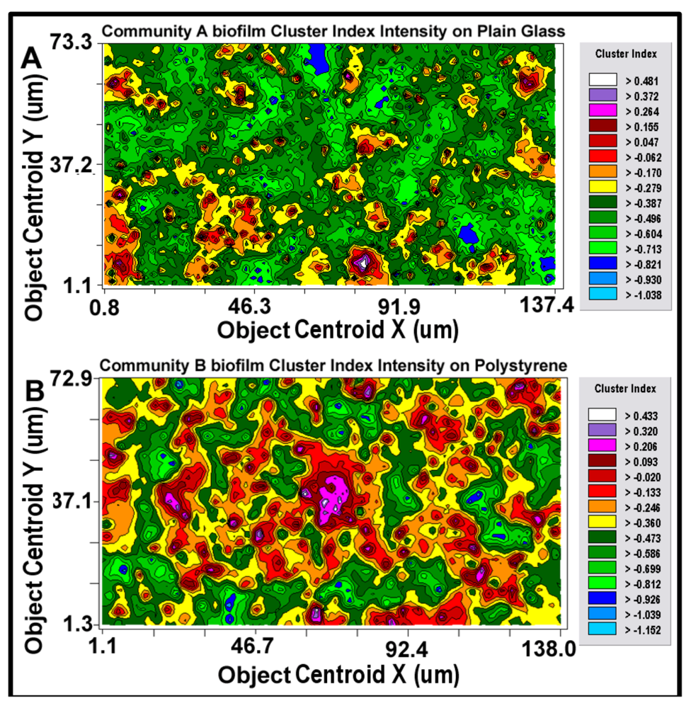
After the best-fit autocorrelation model is computed, the corresponding kriging map can be built (Figure 11a,b). This kriging method uses the best-fit statistical model to estimate values of the quantitative, regionalized Z-variate parameter and provides a vivid, geostatistically defendable continuous interpolation map of the spatial variability of that parameter, even at places where it has not been measured within the entire spatial domain [10,55]. Included in the kriging map are isopleth lines whose curvature connects points of equal value. The configuration of these contours and the pseudocolored scale associated with them reveal the relative gradient of the Z-variate’s intensity of cell–cell interactions within spatially defined clusters, and estimates that parameter at every spatial location within the landscape domain, like weather maps that interpolate the spatial gradients of temperature and cloud cover over large-scale landmasses.

Figure 11. 2-dimensional kriging maps of the spatial heterogeneity in autocorrelated intensity of positive aggregated colonization behavior of the microbial assemblages in the two biofilm landscapes representing community A (a) and B (b). The kriging map legends show the stepped scale of pseudocolored bins that cover the full range of the Z-variate intensity (CMEIAS cluster index) in each landscape.

Amazing to find the many significant differences in ecophysiology between the two biofilm communities despite their development only a few inches apart on the fishing line submerged in the flowing Red Cedar River.

Kriging indicates the statistically defendable, intensity-scaled aggregated colonization behavior over a continuum of radial distances in the biofilm landscapes. The pseudocolored scaling and associated isopleth lines in the modeled kriging map (Figure 11a,b) deliver clearly delineated evidence of autocorrelated centers of highly intensive, local cell–cell aggregation behavior with raised probability of intercellular interactions that are significantly stronger and spatially abundant in the biofilm community B that developed on the polystyrene substratum. These awesome foci of strongly clustered cells colocalize with epicenters of “hot spots” revealed by the point pattern method of linear alignments (Figure 8a,b), and with the georeferenced posting plots of cells represented by bubbles whose widths are weighted by each individual cell’s cluster index (Figure 9a,b). Kriging analysis also predicts the in situ strength of diffusion gradients of extracellular signal molecules that promote/positively regulate these cooperative cell-to-cell interactions within the biofilm [12,49,52].

3.4. Color-Differentiated Microbial Ecophysiology

Many methods of microbial ecophysiology use color differentiation to indicate their in situ status or activities. A significant limitation of this approach is the difficult yet commonplace challenge of removing background pixels whose three-dimensional RGB color space overlaps the range that defines the foreground objects. A CMEIAS Color Segmentation toolkit has been developed to alleviate that problem [14] (available for free download at the CMEIAS website), making it possible to increase the accuracy of measuring ecophysiological attributes of individuals, populations and communities that are differentiated by their color within images. Four ecophysiological applications of this CMEIAS toolkit are illustrated here.

In the first example, color segmentation is used to improve the accuracy in classification of live vs. dead cells of Yersinia pestis based on their color differentiation when stained with the commercial BacLight™ Live/Dead reagent. In theory, live cells should fluoresce green because their intact cell membranes allow passage of only the Syto9 stain that ionically bonds to their nucleoid DNA. In contrast, dead cells should fluorescence red because the propidium iodide reagents used in the protocol can permeate their damaged and leaky membranes, and its higher affinity for DNA should displace the Syto9 stain. In practice however, this classification of cell viability is not always straightforward because some “dead” cells fluoresce yellow because either both stains are intermixed together in the same region within the cell or they occur in distinctly separated red and green regions of fluorescence within the same cell. By applying color segmentation methods to the image example (Figure 12a–c), one finds that nearly half of the proportion of cells that would be visibly scored as “live” (green in Figure 12a) have actually taken up the red-fluorescent propidium iodide stain (Figure 12c) indicating their membranes are fragmented and therefore they are, in reality, “dead”. The Figure 12 table insert indicates the abundant error obtained when “live” cells are scored visually as green despite the presence of intracellular propidium iodide as compared to the correct score of “live” cells with intact membranes.

The second example of color differentiated microbial ecophysiology involves the use of redox stains to mark respiring bacteria and determine what portion of the community is active in oxidative metabolism [11]. Typically, redox-sensitive stains taken up by the bacteria undergo color changes when reduced by respiration using an active electron transport system, and then the entire population is counterstained using a dye of contrasting color. Figure 13a is an example of filter-collected freshwater bacterioplankton cells stained with the redox-sensitive fluorogenic dye 5-Cyano-2, 3-ditolyltetrazolium chloride (CTC) followed by the universal staining dye SYBR^R Gold. In this case, all cells fluoresce blue with SYBR Gold and the actively respiring cells among them accumulate crystals of the reduced formazan product of the CTC electron acceptor that fluoresces red. Note the variation in respiratory activity among individual cells. A problem with direct visual assessment is that some respiring bacteria are scored as false negative because they accumulate insufficient amounts of the red fluorescent product that are obscured by the strong blue fluorescence of the contrasting counterstain, producing a resultant underestimate of the proportion of cells that are actively respiring. This error can be minimized by applying a color segmentation protocol to the digital image (invert color table, increase contrast, split touching cells, split chromatic channels) to produce the resultant second image (Figure 13b). Color-differentiated digital analysis of the magnified image (Figure 13b) corrects the false negative errors, indicating that the proportion of actively respiring cells is significantly higher than what is visibly scored directly in the Figure 13a original image (72% vs. 12%, respectively).

Figure 12. Use of the BacLight™ staining method to differentiate “live” versus “dead” cells of Yersinia pestis after prolonged storage in distilled water. (A) Raw RGB image representing the visual result. (B) and (C) show the same microscope field with chromatic separation of each cell’s emitted fluorescence light using color segmentation methods. Note that many of the green fluorescent cells scored visually as “live” in image A actually have leaky compromised membranes allowing uptake of red-fluorescent propidium iodide (C), and therefore they are “dead”. The table insert provides the erroneous differentiation of viability when only scored visually, and the correct result when this staining method is scored accurately after proper segmentation using CMEIAS color segmentation software.

Figure 13. Use of color segmentation in ecophysiological studies of respiring bacteria. (a) All cells are stained blue with SYBR Gold and the actively respiring bacteria accumulate the CTC-reduced red fluorescent product. (b) The resultant image produced by a color segmentation protocol shows that a much larger percentage of the same cells were actively respiring (accumulated reduced product is now blue) than can be easily recognized by visual counting of cells with red reduced product in the original image (a).

A third example of color-differentiated microbial ecophysiology involves an in situ analysis of phylogenetically based substrate utilization by microbes. This method uses fluorescence in situ hybridization of 16S rRNA oligonucleotide probes combined with microautoradiography (FISH-MAR) to detect metabolically active microbial populations of specific ribotypes within biofilm communities at spatial scales relevant to the bacteria present, thereby directly linking their phylogenetic identity and activity in complex environments [13,48,59,60,61]. The pair of FISH-MAR images used to illustrate this application (Figure 14a,b) was derived from an elegant study to analyze the in situ utilization of (¹⁴C)-labeled pyruvate by two different ribotypes of nitrifying bacteria (Nitrospira and other ammonia oxidizers) in a biofilm developing within a wastewater treatment bioreactor [13]. Accurate color segmentation of Figure 14a produced the output FISH images containing only the foreground object pixels of the two color-differentiated ribotypes (Figure 14c,e), and then these segmented color images were used to isolate selected regions of the corresponding microautoradiography images (Figure 14d,f) containing only the co-localized silver grains of the foreground objects without having to draw the digital areas of interest manually. The ability of the CMEIAS system to perform local-weighted color segmentation made it possible to include the faint single-colored areas selectively while simultaneously avoiding the overlapping double colored areas, thus ensuring that no fluorescent metabolically active biomass was omitted because it did not categorize neatly into either the red or green color channels. In this way, the tedious and potentially inconsistent manual steps were eliminated from the protocol, and the segmented output images accurately retained the size, shape, location and luminosity of the unaltered foreground biofilm cells in a noise-free background [14]. Quantitative image analysis of the color-differentiated FISH-MAR images indicate that the Nitrospira-like ribotype covered approximately one-third as much of the percent biofilm substratum, one-fourth as much of the microdensitometry index (SumGrayIntensity*Area, representing the quantity of assimilated ¹⁴C-pyruvate), and one-half as much of the area-weighted grain intensity (SumGrayIntensity/Area, representing the local intensity of assimilated ¹⁴C-pyruvate) when compared to the corresponding scores for the same metrics associated with the other microprobe-detected nitrifiers.

Figure 14. Application of CMEIAS color segmentation to process images for in situ FISH-MAR in a flattened stack of confocal images of a nitrifying biofilm in a wastewater treatment bioreactor. (a) Multiprobe FISH image of Nitrospira (red) and other ammonia oxidizers (green). Bar is 10 μm. (b) Microautoradiography (MAR) image of active utilization of (¹⁴C)-pyruvate by microbes in the same biofilm. (c,e) Binary images of the red (c) and green (e) fluorescent ribotypes derived from the multiprobe FISH image. (d,f) Accurately segmented grayscale images of silver grain density corresponding to the two distinct ribotypes isolated from the original MAR image. Images are modified from [14].

A fourth example of color differentiated microbial ecophysiology involves the use of engineered sensor strains to measure cell-to-cell communication events resulting in environmentally controlled gene expression in situ. Bacterial participation in cell-to-cell communication occurs successfully when positive or negative interactions are found to be spatially autocorrelated, i.e., structured to operate at spatial scales that extend sufficiently to affect neighboring attached cells [12,52]. Earlier studies [12] using quantitative image analysis showed that the ultimate minimum quorum requirement for N-acyl homoserine lactone (AHL)-mediated cell communication between bacteria during their colonization of plant roots was two individual cells (one producer and one sensor), and the spatial scale of their “calling distances” extended out to a maximum of 78 μm (equivalent to two people talking to each other while standing at opposite goals of a football field). Geostatistical analyses of those quantitative results provided evidence that this type of bacterial communication is governed more by the local spatial positioning of the bacteria within diffusion gradients of the signal molecules they produce rather than by an absolute quorum requirement of high population density [12]. Thus, this bacterial cell–cell interaction is more commonplace in the microbial world than predicted by the dogma that it occurs only where population densities are very high.

Figure 15a is another image from the same experimental system [12] where a wheat rhizoplane landscape is colonized by two different reporter strains of Pseudomonas putida, including red-fluorescent cells of the “AHL-signal source” strain and green-fluorescent cells of the “AHL-signal sensor” strain. Induced expression of Gfp fluorescence by the sensor strain indicates cell-to-cell communication mediated by extracellular AHL signal molecules produced during their colonization of the root. Note the variation in fluorescence intensity of intracellular Gfp among the individually attached bacteria. Figure 15b,c show the corresponding color segmented and grayscale annotated images of the green fluorescent sensor cells used to measure this intensity of cell communication. The variation in gene expression of the sensor strain (Figure 15d) is represented by a multimodal distribution, with at least four different peaks of intensity of bacterial cell-to-cell communication that range between “soft whispers” to “intense shouting” during their colonization of roots. Presumably, individual bacteria were discussing important ecophysiological topics with their neighbors while colonizing the rhizoplane, and they did so with varying intensity!

Figure 15. Variation in intensity of gfp gene expression activated by bacterial cell-to-cell communication between neighboring cells of Pseudomonas putida reporter strains colonized on a wheat root. (a): Laser scanning confocal micrograph of a flattened Z-series of optisections of red-fluorescent “signal source” cells and green-fluorescent “signal sensor” cells communicating with each other via N-acylhomoserine lactones. (b): Green color-segmented and (c) grayscale annotated images derived from Figure 15a to measure the communication response. (d) Frequency distribution of the mean luminosity of Gfp fluorescence per sensor cell as an in situ measure of the variation in intensity of cell-to-cell communication at single-cell resolution.

4. Conclusions

This paper describes 63 different ways that data extracted from digital images using CMEIAS image analysis software can strengthen microscopy-based approaches for understanding the ecophysiology of microorganisms at single-cell resolution and at the dimensions that they occur in situ. Examples evaluated on biofilm assemblages developed on microscope slides submerged during four summer days in a freshwater river ecosystem include the in situ assessments of morphological diversity as an indicator of impacts that substratum physicochemistries have on community structure and niche apportionment, dominance and rarity relationships within morphotype populations, allometric scaling relationships between body size, metabolic activity and growth physiology, stress responses to starvation, environmental disturbance and predation, fractal geometry as an indicator of optimal positioning for efficient utilization of allocated nutrient resources, and biogeography assessments of spatial distribution patterns indicating coaggregation or overdispersed uniformity that deviate from complete spatial randomness. Central to these positive (cooperative) and negative (conflict) interactions are various molecular communication events that regulate genes and biofilm architecture affecting microbial colonization behavior. The modeling of spatial patterns and definition of spatial scales at which they occur as reported here represent crucial steps to understand the ecophysiological functioning of these microbial communities. The significance of these results support the model that microcolony development can help microbial species to coexist while occupying their ecological niche and gaining the cooperative benefits of multi-cellularity within biofilms, that spatial aggregation of a few cells can readily produce a sufficient threshold concentration of signal molecules needed for cells to communicate with each other, and that maintaining honesty in signaling can be avoided when the cells involved are able to grow into microcolonies [12,52,62].

The use of transparent borosilicate glass and polystyrene plastic slides has made it possible to assess the impacts that the substratum exerts on the natural aquatic biofilm communities that develop on them, under conditions where their difference in (physico)chemistry is the only environmental variable in the experiment. A consistent outcome was that the magnitude of these biofilm ecophysiological attributes differed significantly, commonly over a greater spatial scale and with more intensity when developed on the polystyrene substratum compared to plain glass. Spatial patterns in the biofilm assemblage of Community A developed on plain borosilicate glass are mixed, dominated by complete randomness but also some indication of uniformity implicating negative interactions as would predictably occur during intense competition or amensalism amidst lower resource allocation and limited growth physiology, and a small indication of some spatial aggregation. In contrast, spatial patterns of the microbes in the biofilm assemblage of Community B are overwhelmingly dominated by spatial aggregation. The implication of these differences in spatial structure is that the hydrophobic polystyrene substratum itself significantly affects the landscape architecture and ecophysiological activities of the microbial assemblage that developed the biofilm in the freshwater ecosystem. Such information should be considered when designing and interpreting experimental studies using polystyrene microtiter plates to examine genes controlling microbial development of biofilms in natural and managed environments. Computer-assisted microscopy can fill large gaps in studies to define how genetic modification of microbes alters their ability to develop biofilms.

Another major message delivered by these studies is the impact of spatial scale on the ecophysiology of microbial cells in biofilms. Characterizing the spatial scale of these interactions is important because it is a strong determinant of spatial patterns that reflect their colonization behavior. Several of the quantitative results reported here have defined—at (sub)micrometer resolution—the statistically significant, micrometer-to-millimeter scales of the spatial patterns that govern microbial cell–cell interactions in situ within biofilms, reflecting the biogeography of their ecophysiological activities. Consequently, the larger scale at which humans perceive biofilms may have little relevance to the microbial processes resulting in their production.

Finally, the intensity of ecophysiological attributes measured here (including those conducted by populations and communities in rivers, plant rhizoplanes and activated sludge) vary at the individual cell level, emphasizing the importance of using computer-assisted microscopy and digital image processing methods to produce the segmented images that truly represent that variability so that the ecological phenomena can be accurately defined quantitatively at single-cell resolution. In addition, microscopy offers the great advantage of direct visual feedback, which allows one to carefully inspect the samples and minimize the quantification biases inherent to some other methods of community analysis [61]. These microscopy-based methods are also fundamental to modern ecological studies that seek to understand bacterial individuality in order to test the emerging theory of individual-based modeling and ecology, which predicts that single cell variation is a major driver of evolutionary events and the ecological dynamics of population structure and function [14,63,64,65].

Future research on the ecophysiology of microbial communities will continue to benefit by including computer-assisted microscopy at spatial scales that are directly relevant to the ecological niches occupied by individual organisms, and that enable quantitative modeling of their landscape architecture and the local intensities at which cell–cell interactions operate. The software tools of CMEIAS digital image analysis available now and in the near future [1,2,3] are admirably suited for that work.

Conflict of Interest

The authors declare no conflict of interest.

Acknowledgments

Our research to develop CMEIAS image analysis software and apply its computing tools to quantify microbial colonization of roots and other surfaces has been supported by the US-Egypt Science & Technology Joint fund project 58-3148-1-140, the Michigan State University Center for Microbial Ecology, and the NSF Long-Term Ecological Research program at the MSU Kellogg Biological Station. We thank Terry Marsh, Rhena Schulmann, Stephan Gantner and Anton Hartmann, and Holger Daims for providing the original images of Yersinia pestis, freshwater bacterioplankton stained with CTC, Pseudomonas putida sensor strains reporting cell-to-cell communication, and FISH-MAR of nitrifying bacteria, respectively, used in this work. We also thank the CMEIAS research team [1] for their inputs. This paper is dedicated in memory of our friends and colleagues, Rawle Hollingsworth who generously supported CMEIAS research and Bill Costerton who pioneering studies inspired this biofilm research.

References

CMEIAS Center for Microbial Ecology Image Analysis System. Available online: http://cme.msu.edu/cmeias/ (accessed on 22 April 2013).
Dazzo, F.B.; Liu, J.; Gross, C.; Reddy, C.; Monosmith, C.; Philips, N.; Radek, C.; Klemmer, K.; Zhou, J.; Smith, P.; et al. CMEIAS v3.10: Advanced Computational Tools of Image Analysis Software Designed to Strengthen Microscopy-Based Approaches for Understanding Microbial Ecology. In 2013 All Scientists Meeting: Kellogg Biological Station Long-Term Ecological Research Program; Michigan State University: East Lansing, MI, USA, 2013. [Google Scholar]
Liu, J.; Dazzo, F.B.; Glagoleva, O.; Yu, B.; Jain, A. CMEIAS: a computer-aided system for the image analysis of bacterial morphotypes in microbial communities. Microbial Ecol. 2001, 41, 173–194. [Google Scholar]
Henrici, A.T. Studies of freshwater bacteria. I. A direct microscopic technique. J. Bacteriol. 1933, 25, 277–286. [Google Scholar]
Roberts, A.; Withers, P. StatistiXL; Version 1.10; Broadway-Nedlands: Kalamunda, Australia, 2012. [Google Scholar]
Towner, H. EcoStat; Version 1.03; Trinity Software Inc.: Campton, NH, USA, 1999. [Google Scholar]
Krebs, C. Ecological Methodology; Version 7.2; Setauket: New York, NY, USA, 2011. [Google Scholar]
Hammer, O.; Harper, D.A.T.; Ryan, P.D. PAST: Paleontological statistics software package for education and data analysis. Palaeontol. Electron. 2001, 4, 1–9. [Google Scholar]
Species Diversity & Richness IV, Version 4.1.2.1554; Pisces Software: Hants, UK, 2007.
GS+, Version7.0.; Gamma Design Software LLC.: Plainwell, MI, USA, 2004.
Freese, H.M.; Karsten, U.; Schumann, R. Bacterial abundance, activity, and viability in the eutrophic river Warnow, Northeast Germany. Microbial Ecol. 2006, 51, 117–127. [Google Scholar] [CrossRef]
Gantner, S.; Schmid, M.; Dürr, C.; Schuhegger, R.; Steidle, A.; Hutzler, P.R.; Langebartels, C.; Eberl, L.; Hartmann, A.; Dazzo, F.B. In situ spatial scale of calling distances and population density-independent N-acylhomoserine lactone mediated communication by rhizobacteria colonized on plant roots. FEMS Microbiol. Ecol. 2006, 56, 188–194. [Google Scholar]
Daims, H.; Nielsen, J.; Nielsen, P.; Schleifer, K.H.; Wagner, M. In situ characterization of Nitrospira-like nitrite-oxidizing bacteria active in wastewater treatment plants. Appl. Environ. Microbiol. 2001, 67, 5273–5284. [Google Scholar] [CrossRef]
Gross, C.A.; Reddy, C.; Dazzo, F.B. CMEIAS color segmentation: an improved computing technology to process color images for quantitative microbial ecology studies at single-cell resolution. Microbial Ecol. 2010, 59, 400–414. [Google Scholar] [CrossRef]
Folland, I.; Trione, D.; Dazzo, F.B. Accuracy of biovolume formulas for CMEIAS computer-assisted microscopy and body size analysis of morphologically diverse microbial populations and communities. Microbial Ecol. 2013. submitted for publication.. [Google Scholar]
Magurran, A.E. Measuring Biological Diversity; Blackwell Publishing: Malden, MA, USA, 2004. [Google Scholar]
Bergey’s Manual of Determinative Bacteriology, 9th; Holt, J.; Krieg, N.; Sneath, P.; Staley, J.; Williams, S. (Eds.) Williams and Wilkins: Baltimore, MD, USA, 1996.
Hendrick, D.; Peacock, A.; White, D.C. Lipid analyses for viable microbial biomass, community composition, metabolic status, and in situ metabolism. In Manual of Environmental Microbiology, 3rd; Hurst, C., Crawford, R., Garland, J., Lipson, D., Mills, A., Stetzenbach, L., Eds.; American Society for Microbiology Press: Washington, DC, USA, 2007; pp. 112–125. [Google Scholar]
Kunitsky, C.; Osterhout, G.; Sasser, M. Identification of microorganisms using fatty acid methyl ester [FAME] analysis and the MIDI Sherlock Microbial Identification System. In Encyclopedia of Rapid Microbiological Methods, 2nd; Miller, M., Ed.; Davis Healthcare International Publishers: River Grove, IL, USA, 2005; pp. 1–17. [Google Scholar]
Bochner, B. Biolog: modern phenotypic microbial identification. In Encyclopedia of Rapid Microbiological Methods, 2nd; Miller, M., Ed.; Davis Healthcare International Publishers: River Grove, IL, USA, 2005; pp. 55–73. [Google Scholar]
Collins, G.; Kavanagh, S.; McHugh, S.; Connaughton, S.; Kearney, A.; Rice, O.; Carrigg, C.; Scully, C.; Bhreathnach, N.; Mahony, T.; et al. Assessing the black box of microbial diversity and ecophysiology: recent advances through polyphasic experiments. J. Environ. Sci. HealthPart A 2006, 41, 897–922. [Google Scholar] [CrossRef]
Liu, W.; Stahl, D. Molecular approaches for the measurement of density, diversity and phylogeny. In Manual of Environmental Microbiology, 3rd; Hurst, C., Crawford, R., Garland, J., Lipson, D., Mills, A., Stetzenbach, L., Eds.; American Society for Microbiology Press: Washington, DC, USA, 2007; pp. 139–156. [Google Scholar]
Ribosomal Database Project. Available online: http://rdp.cme.msu.edu/ (accessed on 22 April 2013).
Hashsham, S.; Fernandez, A.; Dollhopf, S.; Dazzo, F.B.; Hickey, R.; Tiedje, J.M.; Criddle, C.S. Parallel processing of substrate correlates with greater functional stability in methanogenic bioreactor communities perturbed by glucose. Appl. Environ. Microbiol. 2000, 66, 4050–4057. [Google Scholar] [CrossRef]
Fernandez, A.; Hashsham, S.; Dollhopf, D.; Raskin, L.; Glagoleva, O.; Dazzo, F.B.; Hickey, R.; Tiedje, J.M.; Criddle, C.S. Flexible community structure correlates with stable community function in methanogenic bioreactor communities perturbed by glucose. Appl. Environ. Microbiol. 2000, 66, 4058–4067. [Google Scholar] [CrossRef]
Ritchie, M.E. Scale, Heterogeneity, and the Structure and Diversity of Ecological Communities; Princeton University Press: Princeton, NJ, USA, 2010. [Google Scholar]
Yoshiyama, K.; Klausmeier, C.A. Optimal cell size for resource uptake in fluids: a new facet of resource competition. Am. Nat. 2008, 171, 59–70. [Google Scholar] [CrossRef]
Lambshead, P.J.D.; Platt, H.M.; Shaw, K.M. The detection of differences among assemblages of marine benthic species based on an assessment of dominance and diversity. J. Nat. Hist. 1983, 17, 859–874. [Google Scholar] [CrossRef]
Gaston, K.J. Rarity; Springer: Danvers, MA, USA, 1994. [Google Scholar]
West, G.B.; Woodruff, W.H.; Brown, J.H. Allometric scaling of metabolic rate from molecules and mitochondria to cells and mammals. Proc. Natl. Acad. Sci. USA 2002, 99, 2473–2478. [Google Scholar] [CrossRef]
Baker, R.M.; Singleton, F.L.; Hood, M.A. Effects of nutrient deprivation on Vibrio cholerae. Appl. Environ. Microbiol. 1983, 46, 930–940. [Google Scholar]
Holmquist, L.; Kjelleberg, S. Changes in viability, respiratory activity, and morphology of the marine Vibrio. sp. strain S14 during starvation of individual nutrients and subsequent recovery. FEMS Microbiol. Ecol. 1993, 12, 215–224. [Google Scholar] [CrossRef]
Solow, A.R. A simple test for change in community structure. J. Anim. Ecol. 1993, 62, 191–193. [Google Scholar] [CrossRef]
Tilman, D.; Knops, J.; Wedin, D.; Reich, P.; Ritchie, M.; Siemann, E. The influence of functional diversity and composition on ecosystem processes. Science 1997, 277, 1300–1302. [Google Scholar] [CrossRef]
Shade, A.; Hogan, S.; Klimowicz, A.K.; Linske, M.; McManus, P.S.; Handelsman, J. Culturing captures members of the soil rare biosphere. Environ. Microbiol. 2012, 14, 2247–2252. [Google Scholar] [CrossRef]
Warwick, R.M.; Clarke, K.M. Relearning the ABC: Taxonomic changes and abundance/biomass relationships in disturbed benthic communities. Mar. Biol. 1994, 118, 739–744. [Google Scholar] [CrossRef]
Jürgens, K.; Arndt, H.; Zimmermann, H. Impact of metazoan and protozoan grazers on bacterial biomass distribution in microcosm experiments. Aquat. Microb. Ecol. 1997, 12, 131–138. [Google Scholar] [CrossRef]
Hahn, M.W.; Moore, E.R.; Hofle, M.G. Bacterial filament formation, a defense mechanism againstflagellate grazing, is growth rate controlled in bacteria of different phyla. Appl. Environ. Microbiol. 1999, 65, 25–35. [Google Scholar]
West, G.; Brown, J.; Enquist, B. The fourth dimension of life: fractal geometry and allometric scaling of organisms. Science 1999, 284, 1677–1679. [Google Scholar] [CrossRef]
Hermanowicz, S.; Schindler, U.; Wilderer, P. Fractal structure of biofilms: new tools for investigation of morphology. Water Sci. Technol. 1995, 32, 99–105. [Google Scholar]
Yang, X.; Beyenal, H.; Harkin, G.; Lewandowski, Z. Quantifying biofilm structure using image analysis. J. Microbiol. Meth. 2000, 39, 109–119. [Google Scholar]
Zhou, J.; Ho, J.; Dazzo, F.B. CMEIAS JFrad: a new computing toolkit to discriminate the fractal geometry of landscape architecture and optimal positioning of individual cells for efficient resource allocation in microbial biofilms. Microb. Ecol. 2013. Submitted for publication.. [Google Scholar]
Turner, M.G. Landscape ecology: the effect of pattern on process. Annu. Rev. Ecol. Syst. 1989, 20, 171–197. [Google Scholar]
Hassell, M.P.; May, R.M. Stability in insect host-parasite models. J. Anim. Ecol. 1973, 42, 693–726. [Google Scholar] [CrossRef]
Perry, J. Measures of spatial patterns for counts. Ecology 1998, 79, 1008–1017. [Google Scholar] [CrossRef]
Yanni, Y.G.; Rizk, R.Y.; Abd El-Fattah, F.K.; Squartini, A.; Corich, V.; Giacomini, A.; de Bruijn, F.; Rademaker, J.; Maya-Flores, J.; Ostrom, P.; et al. The beneficial plant growth-promoting association of Rhizobium leguminosarum bv. trifolii with rice roots. Austr. J. Plant Physiol. 2001, 28, 845–870. [Google Scholar]
Dazzo, F.B. Applications of quantitative microscopy in studies of plant surface microbiology. In Plant Surface Microbiology; Varma, A., Abbott, L., Werner, D., Hampp, R., Eds.; Springer-Verlag: Berlin, Germany, 2004; pp. 503–550. [Google Scholar]
Dazzo, F.B.; Schmid, M.; Hartmann, A. Immunofluorescence microscopy and fluorescence in situ hybridization combined with CMEIAS and other image analysis tools for soil- and plant-associated microbial autecology. In Manual of Environmental Microbiology, 3rd; Garland, J., Hurst, C., Lipson, D., Mills, A., Stetzenbach, L., Crawford, R., Eds.; American Society for Microbiology Press: Washington, DC, USA, 2007; pp. 712–733, Chapter 59. [Google Scholar]
Dazzo, F.B.; Yanni, Y.G. CMEIAS: An improved computing technology for quantitative image analysis of root colonization by rhizobacteria in situ at single-cell resolution. In Molecular Microbial Ecology of the Rhizosphere; DeBruijn, F., Ed.; John Wiley & Sons: New York, NY, USA, 2013; Volume 2, pp. 733–742, Chapter 69. [Google Scholar]
Fukuda, M.; Matsuyama, J.; Katano, T.; Nakano, S.; Dazzo, F.B. Assessing primary and bacterial production rates in biofilms on pebbles in Ishite Stream, Japan. Microbial Ecol. 2006, 52, 1–9. [Google Scholar] [CrossRef]
Dazzo, F.B. CMEIAS digital microscopy and quantitative image analysis of microorganisms. In Microscopy: Science, Technology, Applications and Education; Mendez-Vilas, A., Diaz, J., Eds.; Formatex Research Center: Badajoz, Spain, 2010; Microscopy Book Series #4; pp. 1083–1090. [Google Scholar]
Dazzo, F.B. CMEIAS-aided microscopy of the spatial ecology of individual bacterial interactions involving cell-to-cell communication within biofilms. Sensors 2012, 12, 7047–7062. [Google Scholar] [CrossRef]
Ripley, B.D. Tests of “randomness” for spatial point patterns. J. R. Stat. Soc. 1979, 41, 368–374. [Google Scholar]
Hammer, O. New methods for the statistical detection of point patterns. Comput. Geosci. 2009, 35, 659–666. [Google Scholar] [CrossRef]
Robertson, G.P. Geostatistics in ecology: interpolating with known variance. Ecology 1987, 68, 744–748. [Google Scholar] [CrossRef]
Ettema, C.H.; Wardle, D.H. Spatial soil ecology. Trends Ecol. Evol. 2002, 17, 117–183. [Google Scholar]
Dazzo, F.B.; Joseph, A.R.; Gomaa, A.B.; Yanni, Y.G.; Robertson, G.P. Quantitative indices for the autecological biogeography of a Rhizobium endophyte of rice at macro and micro spatial scales. Symbiosis 2003, 35, 147–158. [Google Scholar]
Costerton, J.W. Biofilms. In Topics in Ecological and Environmental Microbiology; Schmidt, T., Schaechter, M., Eds.; Academic Press: Waltham, MA, USA, 2011; pp. 37–42. [Google Scholar]
Lee, N.; Nielsen, P.H.; Andreasen, K.; Juretschko, S.; Nielsen, J.; Schleifer, K.; Wagner, M. Combination of fluorescent in situ hybridization and microautoradiography: A new tool for structure–function analyses in microbial ecology. Appl. Environ. Microbiol. 1999, 65, 1289–1297. [Google Scholar]
Nielsen, J.; Christensen, D.; Kloppenborg, M.; Nielsen, P. Quantification of cell-specific substrate uptake by probe-defined bacteria under in situ conditions by microautoradiography and fluorescence in situ hybridization. Environ. Microbiol. 2003, 5, 202–211. [Google Scholar] [CrossRef]
Daims, H.; Wagner, M. Quantification of uncultured microorganisms by fluorescence microscopy and digital image analysis. Appl. Microbiol. Biotech. 2007, 75, 237–248. [Google Scholar] [CrossRef]
Hense, B.A.; Kuttler, C.; Müller, J.; Rothballer, M.; Hartmann, A.; Kreft, J.-U. Does efficiency sensing unify diffusion and quorum sensing? Nature Rev. Microbiol. 2007, 5, 230–239. [Google Scholar] [CrossRef]
Grimm, V.; Railsback, S.F. Individual-Based Modeling and Ecology; Princeton University Press: Princeton, NJ, USA, 2005. [Google Scholar]
Dethlefsen, L.; Relman, D.A. The importance of individuals and scale: moving towards single-cell microbiology. Environ. Microbiol. 2007, 9, 8–10. [Google Scholar] [CrossRef]
Prosser, J.I.; Bohannan, B.J.; Curtis, T.P.; Ellis, R.J.; Firestone, M.K.; Freckleton, R.P.; Green, J.L.; Green, L.E.; Killham, K.; Lennon, J.J.; et al. The role of ecological theory in microbial ecology. Nat. Rev. Microbiol. 2007, 5, 384–392. [Google Scholar]

© 2013 by the authors; licensee MDPI, Basel, Switzerland. This article is an open access article distributed under the terms and conditions of the Creative Commons Attribution license (http://creativecommons.org/licenses/by/3.0/).

Share and Cite

MDPI and ACS Style

Dazzo, F.B.; Klemmer, K.J.; Chandler, R.; Yanni, Y.G. In Situ Ecophysiology of Microbial Biofilm Communities Analyzed by CMEIAS Computer-Assisted Microscopy at Single-Cell Resolution. Diversity 2013, 5, 426-460. https://doi.org/10.3390/d5030426

AMA Style

Dazzo FB, Klemmer KJ, Chandler R, Yanni YG. In Situ Ecophysiology of Microbial Biofilm Communities Analyzed by CMEIAS Computer-Assisted Microscopy at Single-Cell Resolution. Diversity. 2013; 5(3):426-460. https://doi.org/10.3390/d5030426

Chicago/Turabian Style

Dazzo, Frank B., Kevin J. Klemmer, Ryan Chandler, and Youssef G. Yanni. 2013. "In Situ Ecophysiology of Microbial Biofilm Communities Analyzed by CMEIAS Computer-Assisted Microscopy at Single-Cell Resolution" Diversity 5, no. 3: 426-460. https://doi.org/10.3390/d5030426

APA Style

Dazzo, F. B., Klemmer, K. J., Chandler, R., & Yanni, Y. G. (2013). In Situ Ecophysiology of Microbial Biofilm Communities Analyzed by CMEIAS Computer-Assisted Microscopy at Single-Cell Resolution. Diversity, 5(3), 426-460. https://doi.org/10.3390/d5030426

Article Menu