Diversity-Carbon Flux Relationships in a Northwest Forest


Abstract
:1. Introduction
2. Materials and Methods
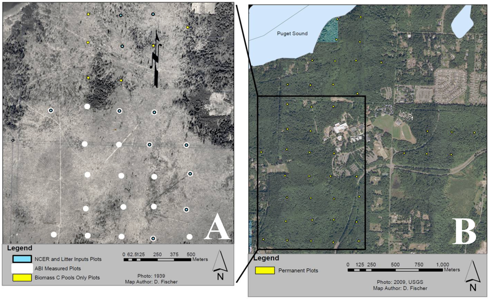
2.1. Study Area

2.2. Soil Nutrients
2.3. Changes in Aboveground Standing Carbon
2.4. Coarse and Fine Woody Debris

| S | n | TPH | SPH | DWDPH | Tree C | Snag C | DWD C | Sap C | FWD C1 | US C | Plot C |
|---|---|---|---|---|---|---|---|---|---|---|---|
| 1 | 2 | 525.48 | 143.31 | 302.55 | 148.05 | 12.01 | 14.86 | 0.06 | 8.62 (2) | 7.31 | 182.29 |
| 2 | 5 | 343.95 | 343.95 | 407.64 | 148.79 | 15.37 | 12.8 | 0.16 | 9.15 (1) | 5.8 | 182.92 |
| 3 | 13 | 443.41 | 210.68 | 440.96 | 236.95 | 5.45 | 22.86 | 0.18 | 8.81 (4) | 3.89 | 269.33 |
| 4 | 16 | 491.64 | 222.93 | 423.97 | 287.21 | 5.84 | 21.72 | 0.17 | 8.01 (4) | 3.97 | 318.91 |
| 5 | 7 | 509.55 | 200.18 | 414.01 | 286.55 | 4.72 | 16.78 | 0.19 | n/a | 5.06 | 321.792 |
| 6 | 1 | 668.79 | 127.39 | 95.54 | 154.35 | 13.2 | 1.25 | 0.32 | n/a | 5.08 | 182.692 |
| Weighted | Ave. | 469.02 | 223.65 | 412.57 | 247.18 | 7.08 | 19.48 | 0.17 | 8.52 | 4.51 | 286.91 |
2.5. Saplings
2.6. Understory Community
2.7. Net Soil CO2 Efflux Rate
2.8. Overstory Richness and Diversity
2.9. Statistical Analysis
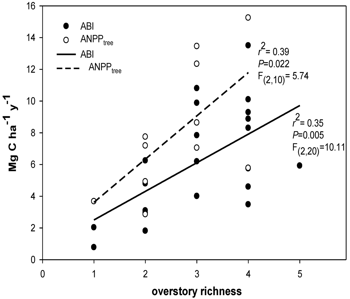
3. Results
3.1. Species Diversity
| Tree C | Snag C | DWD C | Plot C | ABI | ANPPtree | Soil CO2 efflux | |
| n = 44 | n = 44 | n = 44 | n = 44 | n = 21 | n = 11 | n = 11 | |
| Overstory Richness 5 | 0.18, 0.004 | 0.666 | 0.249 | 0.114 | 0.35, 0.005 | 0.39, 0.022 | 0.71, 0.002 |
| Overstory Richness All | 0.074 | 0.364 | 0.837 | 0.175, 0.005 | 0.29, 0.013 | 0.52, 0.013 | 0.41, 0.034 |
| Simpson’s D | 0.131 | 0.071 | 0.622 | 0.177 | 0.26, 0.017 | 0.40, 0.037 | 0.68, 0.002 |
| Shannon’s H’ | 0.116 | 0.111 | 0.747 | 0.193 | 0.30, 0.011 | 0.46, 0.022 | 0.69, 0.002 |
| P. menziesii % dom. | 0.400 | 0.183, 0.004 | 0.737 | 0.326 | 0.093 | 0.404 | 0.123 |
| A rubra % dom. | 0.090 | 0.170 | 0.126 | 0.09, 0.046 | 0.174 | 0.591 | 0.63, 0.004 |
| T. plicata % dom. | 0.721 | 0.138 | 0.269 | 0.774 | 0.734 | 0.960 | 0.534 |
| A. macrophyllum % dom. | 0.448 | 0.540 | 0.327 | 0.408 | 0.548 | 0.553 | 0.775 |
| T. heterophylla % dom. | 0.752 | 0.240 | 0.740 | 0.799 | 0.438 | 0.658 | 0.659 |
| AICc | n | Lik-Model | wi (~probabilities) | Evid. Ratio | ||
|---|---|---|---|---|---|---|
| ABI | ||||||
| Simpson’s D | 59.90 | a | 11 | 1.00 | 0.26 | 1.00 |
| Shannon’s H’ | 60.88 | ab | 11 | 0.61 | 0.16 | 1.64 |
| Intercept Only | 60.89 | ab | 11 | 0.61 | 0.16 | 1.65 |
| Overstory Richness 5 | 61.25 | b | 11 | 0.51 | 0.13 | 1.97 |
| Overstory Richness All | 63.27 | c | 11 | 0.19 | 0.05 | 5.41 |
| NH4+ | 63.33 | c | 11 | 0.18 | 0.05 | 5.56 |
| NO3- | 64.18 | c | 11 | 0.12 | 0.03 | 8.51 |
| NMS Community Similarity | 64.41 | c | 11 | 0.10 | 0.03 | 9.54 |
| T. heterophylla % dom. | 64.57 | c | 11 | 0.10 | 0.03 | 10.35 |
| NO3- + NH4+ | 64.60 | c | 11 | 0.10 | 0.02 | 10.49 |
| P. menziesii % dom. | 64.68 | c | 11 | 0.09 | 0.02 | 10.94 |
| A. macrophyllum % dom. | 64.76 | c | 11 | 0.09 | 0.02 | 11.38 |
| T. plicata % dom. | 64.78 | c | 11 | 0.09 | 0.02 | 11.50 |
| A rubra % dom. | 64.82 | c | 11 | 0.09 | 0.02 | 11.74 |
| All Species | 106.01 | d | 11 | 0.00 | 0.00 | 1.03E + 10 |
| AICc | n | Lik-Model | wi (~probabilities) | Evid. Ratio | ||
| ANPPtree | ||||||
| Shannon’s H’ | 47.46 | a | 8 | 1.00 | 0.27 | 1.00 |
| Simpson’s D | 48.01 | ab | 8 | 0.76 | 0.20 | 1.32 |
| Overstory Richness All | 48.07 | ab | 8 | 0.74 | 0.20 | 1.36 |
| Overstory Richness 5 | 48.19 | ab | 8 | 0.69 | 0.19 | 1.44 |
| Intercept Only | 49.56 | b | 8 | 0.35 | 0.09 | 2.87 |
| NH4+ | 54.05 | c | 8 | 0.04 | 0.01 | 27.00 |
| NMS Community Similarity | 54.73 | c | 8 | 0.03 | 0.01 | 38.02 |
| A. macrophyllum % dom. | 54.88 | c | 8 | 0.02 | 0.01 | 40.83 |
| P. menziesii % dom. | 54.99 | c | 8 | 0.02 | 0.01 | 43.19 |
| A rubra % dom. | 55.04 | c | 8 | 0.02 | 0.01 | 44.31 |
| T. plicata % dom. | 55.05 | c | 8 | 0.02 | 0.01 | 44.59 |
| T. heterophylla % dom. | 55.16 | c | 8 | 0.02 | 0.01 | 46.98 |
| NO3- | 55.16 | c | 8 | 0.02 | 0.01 | 47.14 |
| NO3- + NH4+ | 63.15 | d | 8 | 0.00 | 0.00 | 2554.15 |
| All Species | 133.75 | e | 8 | 0.00 | 0.00 | 5.46E + 18 |
| AICc | n | Lik-Model | wi (~probabilities) | Evid. Ratio | ||
| Net Soil CO2 Efflux | ||||||
| Simpson’s D | 42.18 | a | 10 | 1.00 | 0.50 | 1.00 |
| Shannon’s H’ | 44.36 | b | 10 | 0.34 | 0.17 | 2.97 |
| Overstory Richness 5 | 44.66 | b | 10 | 0.29 | 0.14 | 3.45 |
| A rubra % dom. | 45.33 | b | 10 | 0.21 | 0.10 | 4.82 |
| Overstory Richness All | 46.23 | b | 10 | 0.13 | 0.07 | 7.56 |
| Intercept Only | 50.49 | c | 10 | 0.02 | 0.01 | 63.74 |
| P. menziesii % dom. | 50.71 | c | 10 | 0.01 | 0.01 | 71.11 |
| NMS Community Similarity | 53.12 | d | 10 | 0.00 | 0.00 | 237.68 |
| T. plicata % dom. | 54.16 | d | 10 | 0.00 | 0.00 | 398.23 |
| T. heterophylla % dom. | 54.42 | d | 10 | 0.00 | 0.00 | 454.17 |
| NH4+ | 54.50 | d | 10 | 0.00 | 0.00 | 472.71 |
| NO3- | 54.68 | d | 10 | 0.00 | 0.00 | 516.76 |
| A. macrophyllum % dom. | 54.78 | d | 10 | 0.00 | 0.00 | 542.62 |
| NO3- + NH4+ | 60.09 | e | 10 | 0.00 | 0.00 | 7719.19 |
| All Species | 101.49 | f | 10 | 0.00 | 0.00 | 7.56E + 12 |
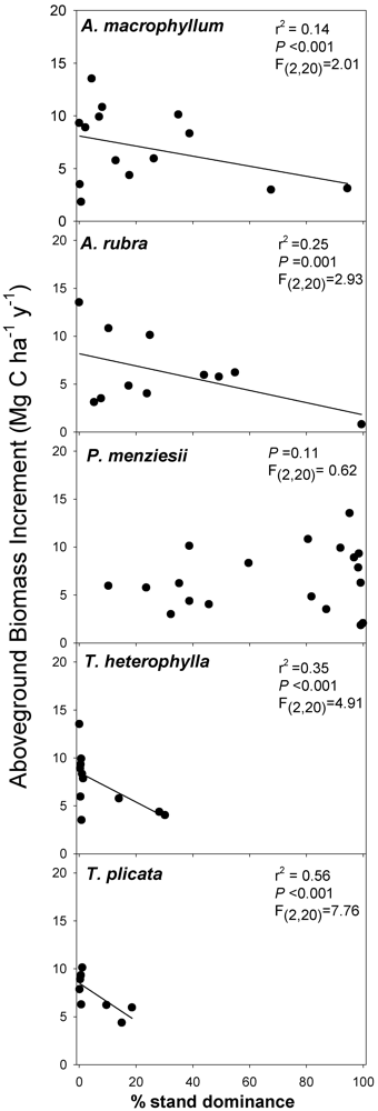
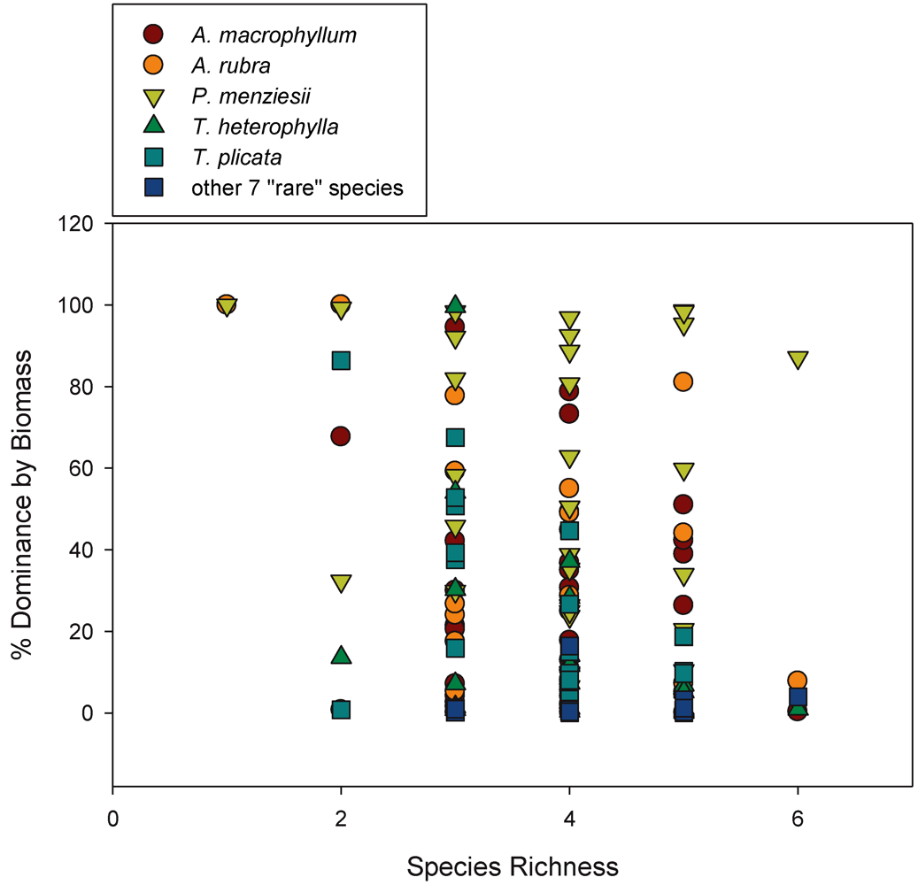
3.2. Biomass-Based Stand Dominance
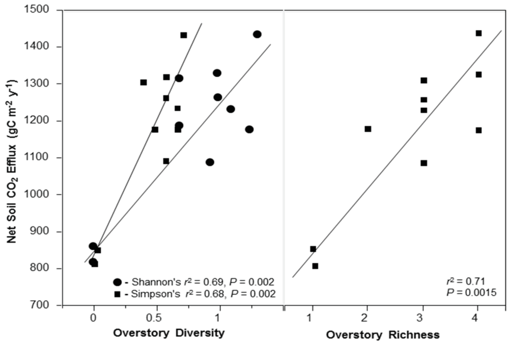
3.3. Net Soil CO2 Efflux
3.4. Soil Nutrients
| C flux/pool | Mineral Soil Chemistry Pool | Pearson Correlation Coefficient | P-value |
| ABI | PO43- | –0.04 | 0.93 |
| ABI | K+ | –0.48 | 0.33 |
| ABI | Ca2+ | –0.06 | 0.91 |
| ABI | % C | 0.09 | 0.87 |
| ABI | NO3- | 0.37 | 0.33 |
| ABI | NH4+ | 0.13 | 0.73 |
| ABI | % Moisture | 0.16 | 0.68 |
| ANPPtree | PO43- | 0.03 | 0.95 |
| ANPPtree | K+ | -0.47 | 0.35 |
| ANPPtree | Ca2+ | -0.06 | 0.91 |
| ANPPtree | % C | 0.04 | 0.94 |
| ANPPtree | NO3- | 0.52 | 0.19 |
| ANPPtree | NH4+ | 0.20 | 0.64 |
| ANPPtree | % Moisture | 0.54 | 0.17 |
| Net Soil CO2 Efflux | PO43- | 0.35 | 0.32 |
| Net Soil CO2 Efflux | K+ | –0.03 | 0.92 |
| Net Soil CO2 Efflux | Ca2+ | 0.29 | 0.41 |
| Net Soil CO2 Efflux | % C | 0.23 | 0.53 |
| Net Soil CO2 Efflux | NO3- | 0.40 | 0.25 |
| Net Soil CO2 Efflux | NH4+ | 0.23 | 0.51 |
3.5. Carbon Pools
4. Discussion
4.1. Carbon Flux and Diversity
4.2. Productivity-Diversity Relationships
4.3. Possible Mechanisms Explaining Productivity-Diversity Relationships
4.4. Net Soil CO2 Efflux and Stand Diversity
4.5. Carbon Pools
4.6. Assumptions and Error
5. Conclusion
Acknowledgements
References
- Schlesinger, W.H. Biogeochemistry: An Analysis Of Global Change; Academic Press: San Diego, CA, USA, 1997; p. 588. [Google Scholar]
- Field, C.B.; Behrenfeld, M.J.; Randerson, J.T.; Falkowski, P. Primary production of the biosphere: integrating terrestrial and oceanic components. Science 1998, 281, 237–240. [Google Scholar]
- Van Tuyl, S.; Law, B.E.; Turner, D.P.; Gitelman, A.I. Variability in net primary production and carbon storage in biomass across Oregon forests—An assessment integrating data from forest inventories, intensive sites, and remote sensing. Forest Ecol. Manag. 2005, 209, 273–291. [Google Scholar]
- Liang, J.; Buongiorno, J.; Monserud, R.A.; Kruger, E.L.; Zhou, M. Effects of diversity of tree species and size on forest basal area growth, recruitment, and mortality. Forest Ecol. Manag. 2007, 243, 116–127. [Google Scholar]
- Keeling, R.F.; Piper, S.C.; Heimann, M. Global and hemispheric CO2 sinks deduced from changes in atmospheric O2 concentration. Nature 1996, 381, 218–221. [Google Scholar]
- Fan, S.; Gloor, M.; Mahlman, J.; Pacala, S.; Sarmiento, J.; Takahashi, T.; Tans, P. A large terrestrial carbon sink in North America implied by atmospheric and oceanic carbon dioxide data and models. Science 1998, 282, 442–446. [Google Scholar]
- Carey, E.V.; Sala, A.; Keane, R.; Callaway, R.M. Are old forests underestimated as global carbon sinks? Glob. Change Biol. 2001, 7, 339–344. [Google Scholar]
- Giardina, C.P.; Coleman, M.D.; Binkley, D.; Hancock, J.E.; King, J.S.; Lilleskov, E.A.; Loya, W.M.; Pregitzer, K.S.; Ryan, M.G.; Trettin, C.C. The response of belowground carbon allocation in forests to global change. In Tree Species Effects on Soils: Implications For Global Change; Binkley, D., Menyailo, O., Eds.; Kluwer Academic: Dordrecht, The Netherlands, 2005; pp. 119–154. [Google Scholar]
- Lieth, H.F.H. Modeling the primary productivity of the world. In Primary Productivity of The Biosphere; Lieth, H.F.H., Whittaker, R.H., Eds.; Ecological Studies 14; Springer-Verlag: Berlin, Germany, 1975; pp. 237–284. [Google Scholar]
- Gholz, H.L. Environmental limits on aboveground net primary production, leaf area, and biomass in vegetation zones of the Pacific Northwest. Ecology 1982, 63, 469–481. [Google Scholar]
- Peterson, D.L.; Waring, R.H. Overview of the Oregon transect ecosystem research project. Ecol. Appl. 1994, 4, 211–225. [Google Scholar]
- Runyon, J.; Waring, R.H.; Goward, S.N.; Welles, J.M. Environmental limits on net primary production and light-use efficiency across the Oregon transect. Ecol. Appl. 1994, 4, 226–237. [Google Scholar]
- Turner, D.P.; Guzy, M.; Lefsky, M.A.; Van Tuyl, S.; Sun, O.; Daly, C.; Law, B.E. Effects of land use and fine-scale environmental heterogeneity on net ecosystem production over a temperate coniferous forest landscape. TELLUS B 2003, 55, 657–668. [Google Scholar]
- Law, B.E.; Turner, D.; Campbell, J.; Sun, O.J.; VanTuryl, S.; Ritts, W.D.; Cohen, W.B. Disturbance and climate effects on carbon stocks and fluxes across Western Oregon, USA. Glob. Change Biol. 2004, 10, 1429–1444. [Google Scholar]
- Boisvenue, C.; Running, S.W. Impacts of climate change on natural forest productivity–evidence since the middle of the 20th Century. Glob. Change Biol. 2006, 12, 1–21. [Google Scholar]
- Swenson, J.J.; Waring, R.H. Modeled photosynthesis predicts woody plant richness at three geographic scales across northwestern USA. Global Ecol. Biogeogr. 2006, 15, 470–485. [Google Scholar]
- Litton, C.M.; Raich, J.W.; Ryan, M.G. Review: Carbon allocation in forest ecosystems. Glob. Change Biol. 2007, 13, 2089–2109. [Google Scholar]
- Litton, C.M.; Giardina, C.P. Belowground carbon flux and partitioning: Global patterns and response to temperature. Funct. Ecol. 2008, 22, 941–954. [Google Scholar]
- Vogel, J.G.; Bond-Lamberty, B.P.; Schuur, E.A.G.; Gower, S.T.; Mack, M.C.; O’Connell, K.B.; Valentine, D.W.; Ruess, R.W. Carbon allocation in boreal black spruce forests across regions varying in soil temperature and precipitation. Glob. Change Biol. 2008, 14, 1503–1516. [Google Scholar]
- Odum, E.P. The strategy of ecosystem development. Science 1969, 164, 262–270. [Google Scholar]
- Loreau, M.; Naeem, S.; Inchausti, P.; Bengtsson, J.; Grime, J.P.; Hector, A.; Hooper, D.U.; Huston, M.A.; Raffaelli, D.; Schmid, B.; Tilman, D.; Wardle, D.A. Biodiversity and ecosystem functioning: current knowledge and future challenges. Science 2001, 294, 804–808. [Google Scholar]
- Fischer, D.G.; Hart, S.C.; LeRoy, C.J.; Whitham, T.G. Variation in belowground carbon fluxes along a Populus hybridization gradient. New Phytol. 2007, 176, 415–425. [Google Scholar]
- Lojewski, N.R.; Fischer, D.G.; Bailey, J.K.; Schweitzer, J.A.; Whitham, T.G.; Hart, S.C. Genetic basis of aboveground productivity in two native Populus species and their hybrids. Tree Physiol. 2009, 29, 1133–1142. [Google Scholar]
- Chapin, F.S.; Woodwell, G.M.; Randerson, J.T.; Rastetter, E.B.; Lovett, G.M.; Baldocchi, D.D.; Clark, D.A.; Harmon, M.E.; Schimel, D.S.; Valentini, R.; Wirth, C.; Aber, J.D.; Cole, J.J.; Goulden, M.L.; Harden, J.W.; Heimann, M.; Howarth, R.W.; Matson, P.A.; McGuire, A.D.; Melillo, J.M.; Mooney, H.A.; Neff, J.C.; Houghton, R.A.; Pace, M.L.; Ryan, M.G.; Running, S.W.; Sala, O.E.; Schlesinger, W.H.; Schulze, E.D. Reconciling carbon-cycle concepts, terminology, and methods. Ecosystems 2006, 9, 1041–1050. [Google Scholar]
- Tilman, D.; Wedin, D.; Knops, J. Productivity and sustainability influenced by biodiversity in grassland ecosystems. Nature 1996, 379, 718–720. [Google Scholar]
- Tilman, D.; Reich, P.B.; Knops, J.; Wedin, D.; Mielke, T.; Lehman, C. Diversity and productivity in a long-term grassland experiment. Science 2001, 294, 843–845. [Google Scholar]
- Naeem, S.; Thompson, L.J.; Lawler, S.P.; Lawton, J.H.; Woodfin, R.M. Declining biodiversity can affect the functioning of ecosystems. Nature 1994, 368, 734–737. [Google Scholar]
- Hector, A.; Schmid, B.; Beierkuhnlein, C.; Caldeira, M.C.; Diemer, M.; Dimitrakopoulos, P.G.; Finn, J.A.; Freitas, H.; Giller, P.S.; Good, J.; Harris, R.; Högberg, P.; Huss-Danell, K.; Joshi, J.; Jumpponen, A.; Körner, C.; Leadley, P.W.; Loreau, M.; Minns, A.; Mulder, C.P.H.; O'Donovan, G.; Otway, S.J.; Pereira, J.S.; Prinz, A.; Read, D.J.; Scherer-Lorenzen, M.; Schulze, E.D.; Siamantziouras, A.S.D.; Spehn, E.M.; Terry, A.C.; Troumbis, A.Y.; Woodward, F.I.; Yachi, S.; Lawton, J.H. Plant diversity and productivity experiments in European grasslands. Science 1999, 286, 1123–1127. [Google Scholar]
- Adams, J.M.; Woodward, F.I. Patterns in tree species richness as a test of the glacial extinction hypothesis. Nature 1989, 339, 699–701. [Google Scholar]
- Scherer-Lorenzen, M.; Körner, C. Forest diversity and function. In Temperate and Boreal Systems; Schulze, E.D., Ed.; Springer: Berlin, Germany, 2005; p. 400. [Google Scholar]
- Naeem, S.; Thompson, L.J.; Lawler, S.P.; Lawton, J.H.; Woodfin, R.M. Biodiversity and ecosystem functioning: Empirical evidence from experimental microcosms. Philos. T. Roy. Soc. B 1995, 347, 249–262. [Google Scholar]
- Aarssen, L.W. High productivity in grassland ecosystems: Effected by species diversity or productive species? Oikos 1997, 80, 183–184. [Google Scholar] [CrossRef]
- Duffy, J.E. Why biodiversity is important to the functioning of real-world ecosystems. Front. Ecol. Environ. 2009, 7, 437–444. [Google Scholar]
- Ellison, A.M.; Bank, M.S.; Clinton, B.D.; Colburn, E.A.; Elliott, K.; Ford, C.R.; Foster, D.R.; Kloeppel, B.D.; Knoepp, J.D.; Lovett, G.M.; Mohan, J.; Orwig, D.A.; Rodenhouse, N.L.; Sobczak, W.V.; Stinson, K.A.; Stone, J.K.; Swan, C.M.; Thompson, J.; von Holle, B.; Webster, J.R. Loss of foundation species: consequences for the structure and dynamics of forested ecosystems. Front. Ecol. Environ. 2005, 9, 479–486. [Google Scholar]
- Scott, N.A.; Binkley, D. Foliage litter quality and net N mineralization: Comparison across North American forest sites. Oecologia 1997, 111, 151–159. [Google Scholar]
- Binkley, D.; Menyailo, O. Tree Species Effects on Soils: Implications for Global Change; Springer: Dordrecht, The Netherlands, 2005; p. 358. NATO Science Series. [Google Scholar]
- Hart, S.C.; Binkley, D.; Perry, D.A. Influence of red alder on soil nitrogen transformations in two conifer forests of contrasting productivity. Soil Biol. Biochem. 1997, 29, 1111–1123. [Google Scholar]
- Bormann, B.T.; Cromack, K.; Russell, W.O. Influences of red alder on soils and long-term ecosystem productivity. In The Biology and Management of Red Alder; Hibbs, D.E., DeBell, D.S., Tarrant, R.F., Eds.; Oregon State University Press: Corvallis, OR, USA, 1994; pp. 47–56. [Google Scholar]
- Comeau, P.G.; Harper, G.J.; Biring, B.S.; Fielder, P.; Reid, W. Effects of red alder on stand dynamics and nitrogen availability (MOF EP1121.01). British Columbia Ministry of Forests and Range Research Branch: Victoria, B.C., Canada, 1997; Extension Note 76. [Google Scholar]
- Deal, R.L.; Harrington, C.A. Red alder: A state of knowledge. In USDA Forest Service General Technical Report; PNW-GTR-669; Pacific Northwest Research Station: Portland, OR, USA, 2006; p. 150. [Google Scholar]
- Tarrant, R.F. Stand development and soil fertility in a Douglas-fir red alder plantation. Forest Sci. 1961, 7, 238–246. [Google Scholar]
- Tarrant, R.F.; Miller, R.E. Accumulation of organic matter and soil nitrogen beneath a plantation of red alder and Douglas-fir. Soil. Sci. Soc. Am. ProC. 1963, 27, 231–234. [Google Scholar]
- Miller, R.E.; Murray, M.D. The effect of red alder on growth of Douglas-fir. In Utilization and Management of Alder; Briggs, D.G., DeBell, D.S., Eds.; USDA Forest Service General Technical Report PNW-FRES-70; USDA Forest Service: Washington, DC, USA, 1978; pp. 283–306. [Google Scholar]
- Binkley, D.; Sollins, P.; Bell, R.; Sachs, D. Biogeochemistry of adjacent conifer and alder-conifer stands. Ecology 1992, 73, 2022–2033. [Google Scholar]
- Van Breeman, N.; Finzi, A.C. Plant-soil interactions: Ecological aspects and evolutionary implications. Biogeochemistry-US 1998, 42, 1–19. [Google Scholar] [CrossRef]
- Spears, J.D.H.; Lajtha, K.; Caldwell, B.A.; Pennington, S.B.; Vanderbilt, K. Species effects of Ceanothus velutinus versus Pseudotsuga menziesii, Douglas-fir, on soil phosphorus and nitrogen properties in the Oregon Cascades. Forest Ecol. Manag. 2001, 149, 205–216. [Google Scholar]
- Selmants, P.; Hart, S.C.; Boyle, S.I.; Stark, J.M. Red alder (Alnus rubra) alters community-level soil microbial function in conifer forests of the Pacific Northwest, USA. Soil Biol. Biochem. 2005, 37, 1860–1868. [Google Scholar]
- Clark, D.A.; Brown, S.; Kicklighter, D.W.; Chambers, J.Q.; Thomlinson, J.R.; Ni, J. Measuring net primary production in forests: Concepts and field methods. Ecol. Appl. 2001, 11, 356–370. [Google Scholar]
- Johnson, D.; Phoenix, G.K.; Grime, G.P. Plant community composition, not diversity, regulates soil respiration in grasslands. Biol. Lett. 2008, 4, 345–348. [Google Scholar]
- TESC Scientific Computing Weather Station. 2011. Available online: http://scicomp.evergreen.edu/ (accessed on 22 March 2011).
- USDA Natural Resources Conservation Service. Web Soil Survey. USDA-Natural Resources Conservation Service: Washington, DC, USA, 2011. Available online: http://websoilsurvey.nrcs.usda.gov/ (accessed on 29 June 2011).
- Nezat, C.A.; Blum, J.D.; Klaue, A.; Johnson, C.E.; Siccama, T.G. Influence of landscape position and vegetation on long-term weathering rates at the Hubbard Brook Experimental Forest, New Hampshire, USA. Geochimica et Cosmochimica Acta 2004, 68, 3065–3078. [Google Scholar]
- Robertson, G.P.; Wedin, D.; Groffman, P.M.; Blair, J.M.; Holland, E.A.; Nadelhoffer, K.J.; Harris, D. Soil carbon and nitrogen availability. In Standard Soil Methods for Long-Term Ecological Research; Robertson, G.P., Ed.; Oxford University Press: New York, NY, USA, 1999; pp. 258–271. [Google Scholar]
- Cairns, M.A.; Brown, S.; Helmer, E.H.; Baumgardner, G.A. Root biomass allocation in the world’s upland forests. Oecologia 1997, 111, 1–11. [Google Scholar] [CrossRef]
- McGaughey, R.J.; Carson, W.W.; Reutebuch, S.E.; Andersen, H.E. Direct measurement of individual tree characteristics from LiDAR data. In Proceedings of the Annual ASPRS Conference, Denver, American Society of Photogrammetry and Remote Sensing, Bethesda, MD, USA, 2004.
- USDA Forest service. Available online: http://www.fs.fed.us/eng/rsac/fusion/ (accessed on 25 April 2010).
- Standish, J.T.; Manning, G.H.; Demaershalk, J.P. Development of biomass equations for British Columbia tree species. Inf. Rep. BC-X-264. Canadian Forestry Service, Pacific Forest Research Center: Victoria, BC, Canada, 1985; p. 48. [Google Scholar]
- Means, J.E.; Hansen, H.A.; Koerper, G.J.; Alaback, P.B.; Klopsch, M.W. Software for computing plant biomass—BIOPAK user’s guide. USDA Forest Service General Technical Report PNW-GTR-340. Pacific Northwest Research Station: Portland, OR, USA, 1994; p. 180. [Google Scholar]
- Gholz, H.L. Equations for estimating biomass and leaf area of plants in the Pacific Northwest. Forest Research Lab., Oregon State University, School of Forestry: Corvallis, OR, USA, 1979. [Google Scholar]
- Harmon, M.E.; Sexton, J. Guidelines for measurements of woody debris in forest ecosystems. Publications No. 2255. U.S. LTER Network Office, University of Washington: Seattle, WA, USA, 1996; p. 73. [Google Scholar]
- Maser, C.; Anderson, R.G.; Ralph, G.; Cromack, K.; Williams, J.T.; Martin, R.E. Dead and down woody material. In Wildlife Habitats in Managed Forests: The Blue Mountains of Oregon and Washington; Thomas, J.W., Ed.; US Forest Service: Washington, DC, USA, 1979; Volume No. 553, pp. 22–39. [Google Scholar]
- McCune, B.; Grace, J.B. Analysis of Ecological Communities; MjM Software: Gleneden Beach, OR, USA, 2002; p. 304. [Google Scholar]
- Burnham, K.P.; Anderson, D.R. Model Selection and Multimodel Inference; A Practical Information-Theoretic Approach; Springer-Verlag: New York, NY, USA, 2002; p. 488. [Google Scholar]
- Hanson, P.J.; Edwards, N.T.; Garten, C.T.; Andrews, J.A. Separating root and soil microbial contributions to soil respiration: A review of methods and observations. Biogeochemistry-US 2000, 48, 115–146. [Google Scholar] [CrossRef]
- Högberg, P.; Nordgren, A.; Buchmann, N.; Taylor, A.F.S.; Ekblad, A.; Högberg, M.; Nyberg, G.; Ottosson-Löfvenius, M.; Read, D.J. Large-scale forest girdling shows that current photosynthesis drives soil respiration. Nature 2001, 411, 789–792. [Google Scholar]
- Raich, J.W.; Schlesinger, W.H. The global carbon dioxide flux in soil respiration and its relationship to vegetation and climate. Tellus B 1992, 44, 81–99. [Google Scholar]
- Craine, J.M.; Wedin, D.A.; Reich, P.B. The response of soil CO2 flux to changes in atmospheric CO2, nitrogen supply and plant diversity. Glob. Change Biol. 2001, 7, 947–953. [Google Scholar]
- Zak, D.R.; Holmes, W.E.; White, D.C.; Peacock, A.D.; Tilman, D. Plant diversity, soil microbial communities and ecosystem function: Are there any links? Ecology 2003, 84, 2042–2050. [Google Scholar] [CrossRef]
- De Boeck, H.J.; Lemmens, C.M.; Vicca, S.; Van den Berge, J.; Van Dongen, S.; Janssens, I.A.; Ceulemans, R.; Nijs, I. How do climate warming and species richness affect CO2 fluxes in experimental grasslands? New Phytologist 2007, 175, 512–522. [Google Scholar] [CrossRef]
- Campbell, J.L.; Sun, O.J.; Law, B.E. Supply-side controls on soil respiration among Oregon forests. Glob. Change Biol. 2004, 10, 1857–1869. [Google Scholar]
- Lyr, H.; Hoffman, G. Growth rates and growth periodicity of tree roots. Int. Rev. Forest. Res. 1967, 2, 181–236. [Google Scholar]
© 2012 by the authors; licensee MDPI, Basel, Switzerland. This article is an open-access article distributed under the terms and conditions of the Creative Commons Attribution license (http://creativecommons.org/licenses/by/3.0/).
Share and Cite
Kirsch, J.L.; Fischer, D.G.; Kazakova, A.N.; Biswas, A.; Kelm, R.E.; Carlson, D.W.; LeRoy, C.J. Diversity-Carbon Flux Relationships in a Northwest Forest. Diversity 2012, 4, 33-58. https://doi.org/10.3390/d4010033
Kirsch JL, Fischer DG, Kazakova AN, Biswas A, Kelm RE, Carlson DW, LeRoy CJ. Diversity-Carbon Flux Relationships in a Northwest Forest. Diversity. 2012; 4(1):33-58. https://doi.org/10.3390/d4010033
Chicago/Turabian StyleKirsch, Justin L., Dylan G. Fischer, Alexandra N. Kazakova, Abir Biswas, Rachael E. Kelm, David W. Carlson, and Carri J. LeRoy. 2012. "Diversity-Carbon Flux Relationships in a Northwest Forest" Diversity 4, no. 1: 33-58. https://doi.org/10.3390/d4010033
APA StyleKirsch, J. L., Fischer, D. G., Kazakova, A. N., Biswas, A., Kelm, R. E., Carlson, D. W., & LeRoy, C. J. (2012). Diversity-Carbon Flux Relationships in a Northwest Forest. Diversity, 4(1), 33-58. https://doi.org/10.3390/d4010033