Article

Simulating the Phylogenetic Diversity Metrics of Plant Communities in Alpine Grasslands of Xizang, China

1
State Key Laboratory of Plateau Ecology and Agriculture, Qinghai University, Xining 810018, China
2
Lhasa Plateau Ecosystem Research Station, Key Laboratory of Ecosystem Network Observation and Modeling, Institute of Geographic Sciences and Natural Resources Research, Chinese Academy of Sciences, Beijing 100101, China
*
Author to whom correspondence should be addressed.
These authors contributed equally to this work.
Diversity 2025, 17(8), 569; https://doi.org/10.3390/d17080569
Submission received: 7 July 2025 / Revised: 4 August 2025 / Accepted: 12 August 2025 / Published: 14 August 2025

Abstract

Phylogenetic diversity serves as a critical complement to traditional species diversity metrics. However, the performance variations among different computational models in simulating phylogenetic diversity within plant communities in the alpine grasslands of the Qinghai-Xizang Plateau remain insufficiently characterized. Here, we evaluated nine modeling approaches—random forest (RF), generalized boosting regression (GBR), multiple linear regression (MLR), artificial neural network (ANN), generalized linear regression (GLR), conditional inference tree (CIT), extreme gradient boosting (eXGB), support vector machine (SVM), and recursive regression tree (RRT)—for predicting three key phylogenetic diversity metrics [Faith’s phylogenetic diversity (PD), mean pairwise distance (MPD), mean nearest taxon distance (MNTD)] using climate variables and NDVImax. Our comprehensive analysis revealed distinct model performance patterns under grazing vs. fencing regimes. The eXGB algorithm demonstrated superior accuracy for fencing conditions, achieving the lowest relative bias (−0.08%) and RMSE (9.54) for MPD, along with optimal performance for MNTD (bias = 2.95%, RMSE = 44.86). Conversely, RF emerged as the most robust model for grazing scenarios, delivering the lowest bias (−1.63%) and RMSE (16.89) for MPD while maintaining strong predictive capability for MNTD (bias = −1.09%, RMSE = 27.59). Notably, scatterplot analysis revealed that only RF, GBR, and eXGB maintained symmetrical distributions along the 1:1 line, while other models showed problematic one-to-many value mappings or asymmetric patterns. These findings show that machine learning (especially RF and eXGB) enhances phylogenetic diversity predictions by integrating climate and NDVI data, though model performance varies by metric and management context. This study offers a framework for ecological forecasting, emphasizing multi-metric validation in biodiversity modeling.

1. Introduction

Plant community phylogenetic diversity, including Faith’s phylogenetic diversity, mean pairwise distance, and mean nearest taxon distance, represents the cumulative branch length of species within a community on a phylogenetic tree [1], serving as a crucial complement to traditional species diversity metrics. In the context of rangeland conservation, phylogenetic diversity provides unique insights into the evolutionary resilience of ecosystems under anthropogenic pressures like grazing and fencing—key management strategies for sustainable pastoralism. Compared with traditional indicators that focus merely on the number of species, phylogenetic diversity provides insights into the evolutionary heterogeneity and functional potential of species within a community. It offers distinct advantages in elucidating the mechanisms of community assembly, ecological processes, and ecosystem functioning [2]. Phylogenetic diversity also plays a crucial role in key conservation [3] and restoration efforts [4], including the identification of priority areas for biodiversity protection and the evaluation of ecological restoration outcomes. Specifically for alpine rangelands, which cover 40% of the Qinghai-Tibet Plateau and face escalating climate and land-use pressures, phylogenetic metrics are critical for assessing conservation priorities under contrasting management regimes. Therefore, investigating the phylogenetic diversity of plant communities not only enhances our understanding of the underlying mechanisms governing community assembly and functional stability, but also offers theoretical foundations and decision support frameworks for ecological conservation, restoration management, and global change research.
Recently, advancements in ecological modeling and data science have led to the widespread application of model simulation techniques in the study of phylogenetic diversity [5,6]. Our focus on alpine grasslands—a system where grazing exclusion (fencing) and traditional pastoralism create stark ecological contrasts—necessitates modeling approaches capable of capturing these management-driven phylogenetic patterns. For example, early studies predominantly employed conventional statistical methods—such as multiple linear regression, generalized linear models, and redundancy analysis—to investigate the relationships between phylogenetic diversity and environmental variables (e.g., climate, hydrology, soil properties, and land use patterns) [7]. Although these models offer strong explanatory power and interpretability, they have limited capacity to capture nonlinear relationships and variable interactions, which restricts their effectiveness in handling high-dimensional and heterogeneous data from complex ecosystems. Furthermore, with advances in spatial ecological modeling, species distribution models, such as MaxEnt, BIOMOD, and ecological niche models, have increasingly been applied to spatial prediction studies of phylogenetic diversity [8]. These approaches infer the geographic patterns of phylogenetic diversity based on species’ spatial distribution data [9]. However, these models are usually established at the species level, neglecting the direct modeling ability of phylogenetic relationships among species within communities.
The choice to model phylogenetic (rather than functional or taxonomic) diversity stems from its unique capacity to (1) reflect deep evolutionary legacies that constrain community responses to management; (2) provide proxy measures of unmeasured functional traits via phylogenetic signal; and (3) identify conservation priorities for evolutionarily distinct lineages. Recently, machine learning models like random forests, XGBoost, SVMs, and ANNs have become widely used in phylogenetic diversity studies due to their ability to handle complex ecological data, model nonlinear relationships, and assess variable importance. For example, Cadotte et al. (2017) proposed that ensemble learning methods can effectively assess the impacts of ecological processes, such as environmental filtering and competitive interactions, on phylogenetic diversity [10]. In recent decades, numerous studies have increasingly sought to integrate multiple algorithms to enhance the robustness of predictive models [11]. Despite continuous advancements in model simulation technology, research on plant community phylogenetic diversity still faces several challenges as follows: firstly, the lack of high-resolution and comprehensive phylogenetic tree data; secondly, inconsistent applicability of various algorithms to community-scale phylogenetic structure indices, such as PD, MPD, and MNTD; thirdly, alpine grasslands exhibit high climate sensitivity [12], and the mechanisms underlying changes in their phylogenetic diversity are complex. Our study specifically targets the Qinghai-Tibet Plateau’s Stipa-Carex-Kobresia dominated ecosystems (28–38° N, 80–100° E; 3000–5000 m elevation), where grazing/fencing contrasts create natural laboratories for testing model performance under real-world conservation scenarios. Therefore, a comprehensive analysis of the response characteristics of plant community phylogenetic diversity under various management scenarios—such as fencing and grazing—in alpine grasslands is essential for elucidating the mechanisms underlying grassland community assembly, maintaining ecological functions, and developing sustainable management strategies.
In this study, the metrics of plant community phylogenetic diversity—including phylogenetic diversity (PD), mean pairwise distance (MPD), and mean nearest taxon distance (MNTD)—were computed using remote sensing and climatic variables such as the normalized difference vegetation index, temperature, precipitation, and solar radiation. These computations were carried out employing nine data mining techniques: random forest, generalized boosted regression, support vector machine, multiple linear regression, recursive regression tree, artificial neural network, generalized linear regression, conditional inference tree, and extreme gradient boosting. The central aim of this research was to assess and compare the predictive accuracy of these modeling approaches in estimating plant community phylogenetic diversity under contrasting rangeland management strategies, thereby bridging the gap between computational ecology and practical conservation decision making.

2. Materials and Methods

2.1. Study Area and Plant Sampling

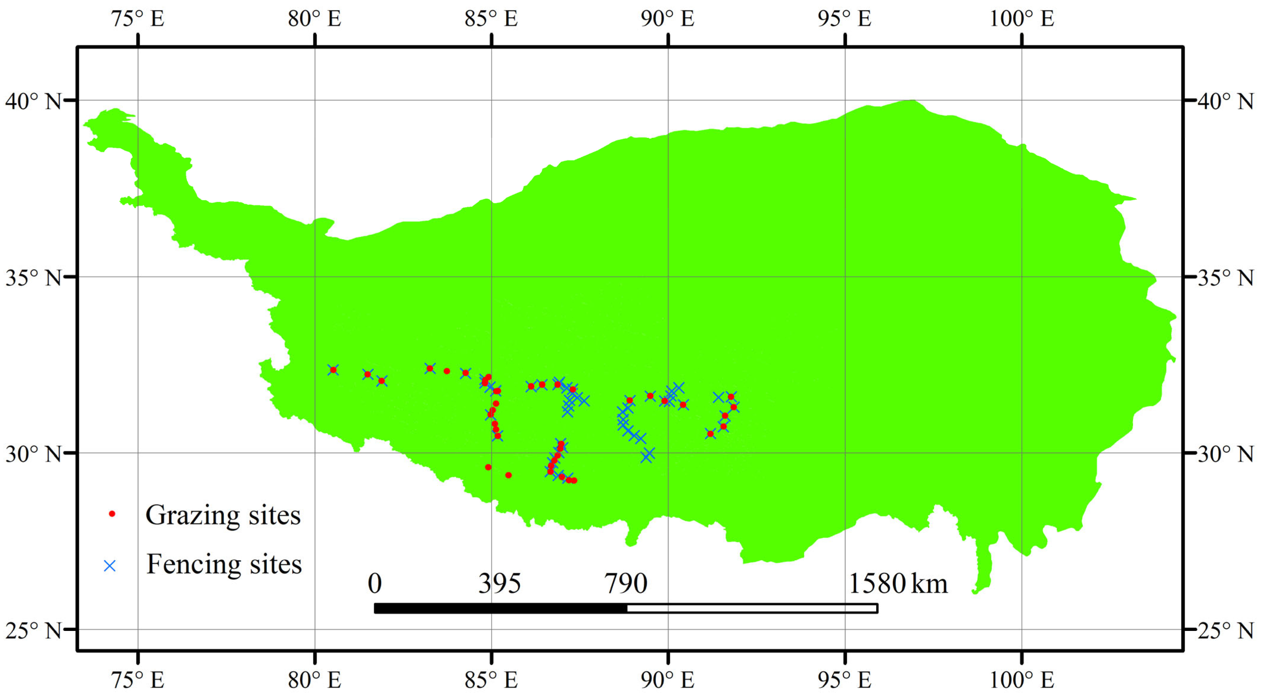
This research was conducted in the Xizang alpine grasslands, China (Figure A1), an area characterized by a plateau monsoon climate with warm and humid summers and cold dry winters, during which the majority of annual precipitation (from 100 to 700 mm) occurs [12]. The region encompasses 1.2 × 10⁶ km2 of alpine grasslands, representing nearly two-thirds of China’s total alpine grassland area, and supports extensive alpine meadow and alpine steppe vegetation, which is typically found at elevations ranging from 3800 to 5200 m [13]. The dominant species include Stipa capillacea, Carex atrofusca, Kobresia pygmaea, and Stipa purpurea. These accelerated climate changes make the Qinghai-Xizang Plateau an ideal system for examining how phylogenetic diversity patterns respond to environmental changes under different management regimes [14].
During the 2020–2021 growing seasons, a stratified random sampling design was implemented across the alpine ecotone, encompassing both meadow and steppe vegetation types (Figure A1). Consistent with vegetation structure differences, nested quadrat systems were employed—0.25 m2 for dense meadow communities versus 1 m2 for open steppe formations—adhering to IUCN ecosystem monitoring guidelines. The investigated plant community data included species richness (number of species per plot), total vegetation cover (%), and mean plant height (cm), recorded during peak growing season. Data were collected from fixed sampling plots using standardized quadrat surveys, ensuring consistent measurement across different management regimes and ecological gradients. These community-level attributes were used to assess vegetation structure and diversity under varying environmental and anthropogenic conditions. Based on the surveyed plant community data, three metrics of phylogenetic diversity were calculated for each sampling quadrat: PD, MPD, and MNTD. These metrics were derived from species composition data and a phylogenetic tree constructed from the regional species pool, enabling quantitative assessment of phylogenetic diversity patterns within plant communities. Phylogenetic diversity metrics, including PD, MPD, and MNTD, were computed using the “picante” package in R, based on species occurrence data per quadrat and a pruned phylogenetic tree tailored to the regional flora. A total of 403 and 226 quadrat-level observations were available for PD, MPD, and MNTD under fencing and grazing conditions, respectively.

2.2. Normalized-Difference Vegetation Index and Climate

The growing-season (May-September) NDVImax data (30 m resolution) were obtained from the National Ecosystem Science Data Center of China [15] (http://www.nesdc.org.cn; accessed on 10 July 2024). Climate variables—annual mean temperature, annual precipitation, and annual radiation—were derived from the National Tibetan Plateau Data Center [https://data.tpdc.ac.cn/zh-hans/data/44a449ce-e660-44c3-bbf2-31ef7d716ec7 (accessed on 2 April 2025)] [16]. The data time span of NDVImax and climate variables was 2000–2021. In exclosure-based models, the three climate variables served as key predictors. For grazing scenarios, NDVImax was incorporated alongside climate variables to specifically capture vegetation productivity responses to grazing pressure, which may modify microclimate conditions and nutrient cycling within pastoral systems.

2.3. Model Methodology

Our sampling design employed stratified randomization (R caret::createDataPartition) with strata defined by (i) land use intensity (continuous grazing vs. long-term fencing >10 years) and (ii) floristic assemblages (verified by NMDS ordination). This approach ensured proportional representation of both anthropogenic treatments and ecological variability. A 75%:25% split was applied within each stratum to generate training and validation subsets. The validation set [n = 50 (grazing); n = 80 (fencing)] preserved stratum balance while minimizing spatial autocorrelation through (1) geographic dispersion of sampling quadrats (Figure A1), ensuring no two validation points fell within 500 m of each other; (2) stratified random selection constrained by environmental covariates (elevation, slope, NDVI). This approach prevented data leakage while maintaining taxonomic representativeness. Sample sizes differed between management regimes (fenced: n = 323; grazed: n = 216) but were balanced across all phylogenetic diversity indices (PD, MNTD, MPD). The distribution reflected natural heterogeneity in grazing pressure and vegetation recovery stages.
All statistical modeling was implemented in R using established discipline-specific packages [17]. (1) Regression-based methods: Multiple linear regression ((MLR); base R stats package) provides a simple interpretable approach for linear relationships [18]. Generalized linear regression (GLR) extends MLR for non-normal error distributions. (2) Tree-based methods: Recursive regression trees ((RRTs); “rpart” package [18]) and conditional inference trees (CITs) partition the feature space recursively to handle nonlinear/high-dimensional data. Random forest ((RF); “randomForest” package [19]) uses parallel ensembles of decision trees to reduce overfitting and assess variable importance. Generalized boosted regression ((GBR); “gbm” package [20]) builds trees sequentially to correct residuals and capture complex patterns. eXtreme gradient boosting ((eXGB); “rminer” package [21]) refines boosting via regularization for improved speed/accuracy. (3) Other machine learning approaches: Support vector machines ((SVMs); “e1071” package [22]) optimize hyperplane placement to maximize classification margins. Artificial neural networks ((ANNs); “rminer” package [21]) simulate biological neural systems to learn intricate nonlinear relationships. Together, these approaches encompass ensemble learning (RF, GBR, eXGB), geometric optimization (SVM), statistical regression (MLR, GLR), rule-based partitioning (RRT, CIT), and adaptive learning (ANN) [23]. This methodological diversity, verified through version control, enables robust modeling across varied data structures while enhancing predictive performance.

2.4. Model Accuracy Evaluation

Quantification of training error varied across modeling frameworks due to differences in R package (version 4.2.2 for windows) implementations. The random forest (RF) model optimized performance by minimizing mean squared error (MSE) and reporting R2-values (Table A1). In contrast, the GBR model employed both mean training error and cross-validation thresholds as stopping criteria (Table A2). Support vector machine (SVM) evaluations focused on residual distributions and hyperplane distances (Table A3), while multiple linear regression (MLR) and recursive regression tree (RRT) relied exclusively on R2 optimization (Table A4 and Table A5). Other models, including GLR, ANN, CIT, and eXGB, used model-specific error reduction protocols (Table A6). To enable consistent comparison across models, we applied four standardized validation metrics: relative bias (quantifying systematic over-/under-prediction), root mean squared error (RMSE, measuring overall deviation magnitude), regression slope of observed vs. simulated values (assessing proportional consistency), and R2 between predicted and observed values (evaluating variance explanation). This suite balances sensitivity to different error types while aligning with standard practices in ecological modeling.

3. Results

3.1. Model Construction

Ensemble models (tree-based aggregations) exhibited systematically distinct structural configurations compared with individual learners across all tested architectures. Our analysis incorporated 629 quadrat-level observations (403 fenced, 226 grazed), ensuring robust statistical comparisons. Under fencing conditions, the number of trees in the RF models ranged from 512 to 623 (Table A1), placing them between the nearly saturated forests of GBR (1000 trees, Table A2) and the kernel-based SVM (280–285 support vectors). Under grazing conditions, RF models contained 723 to 738 trees (Table A1), which was comparable to the GBR models (996–1000 trees, Table A2) but noticeably higher than the number of support vectors in the SVM models (176–192, Table A3). Intrinsic ensemble models, particularly the tree aggregation mechanisms employed in RF, demonstrated consistently superior simulation accuracy across various management regimes (Table A1, Table A4 and Table A5). Under fencing conditions, RF achieved notably higher simulation accuracy (R2 = 0.66–0.72; Table A1) compared with multiple linear regression (R2 = 0.18–0.23; Table A4) and recursive regression (R2 = 0.48–0.54; Table A5). Similarly, under grazing conditions, RF maintained its advantage (R2 = 0.68–0.78; Table A1), outperforming both multiple linear regression (R2 = 0.22–0.29; Table A4) and recursive regression (R2 = 0.22–0.35; Table A5). Training errors showed a degree of computational homogeneity across ANN, GLR, CIT, and eXGB algorithms (Table A6). Under fenced conditions, eXGB consistently yielded the lowest training errors (ranging from 1517.4 to 8771.17) in most scenarios. Under grazing conditions, notable differences in training error were also observed among the ANN, GLR, CIT, and eXGB models (Table A6).

3.2. Model Validation

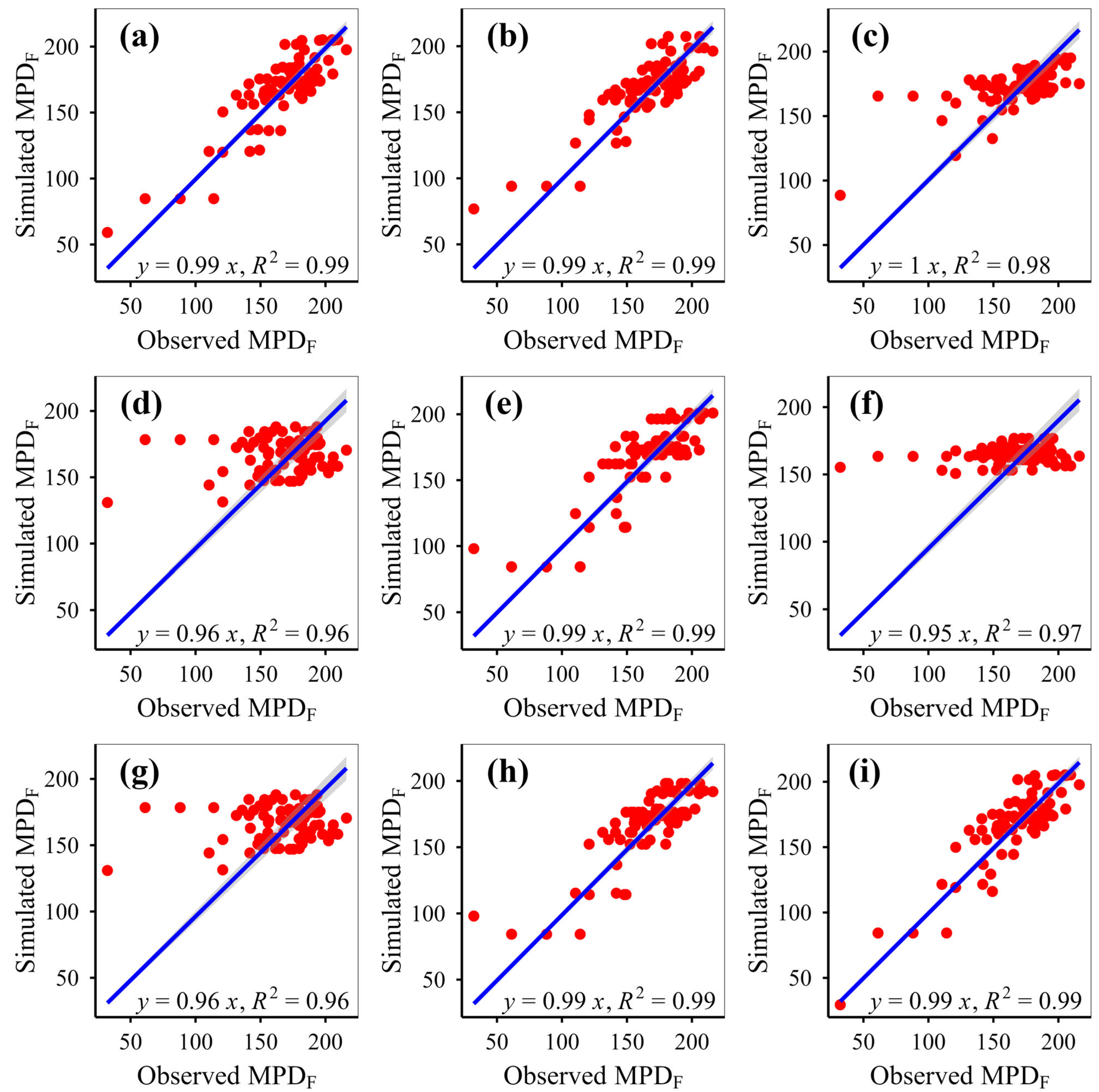
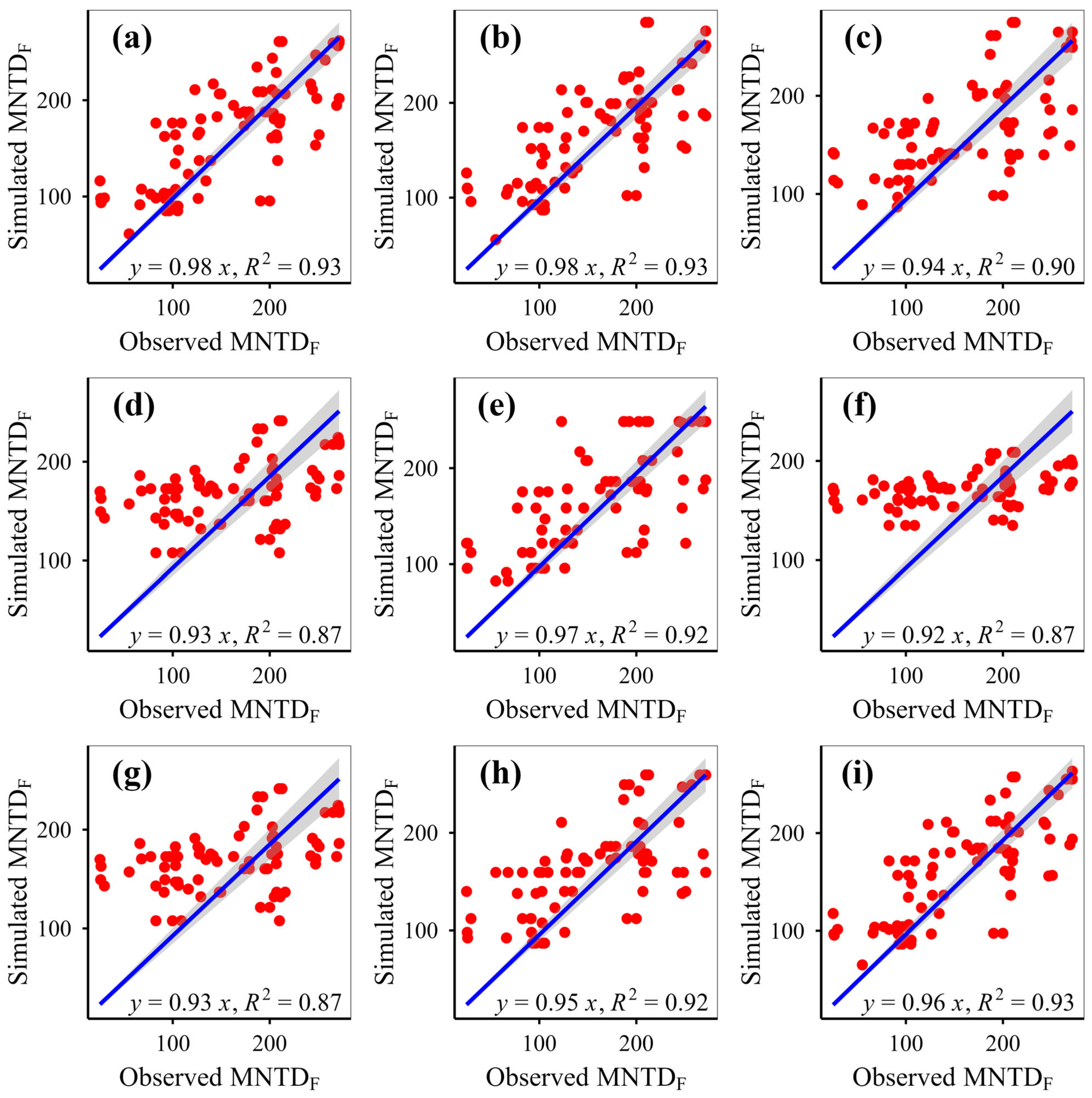
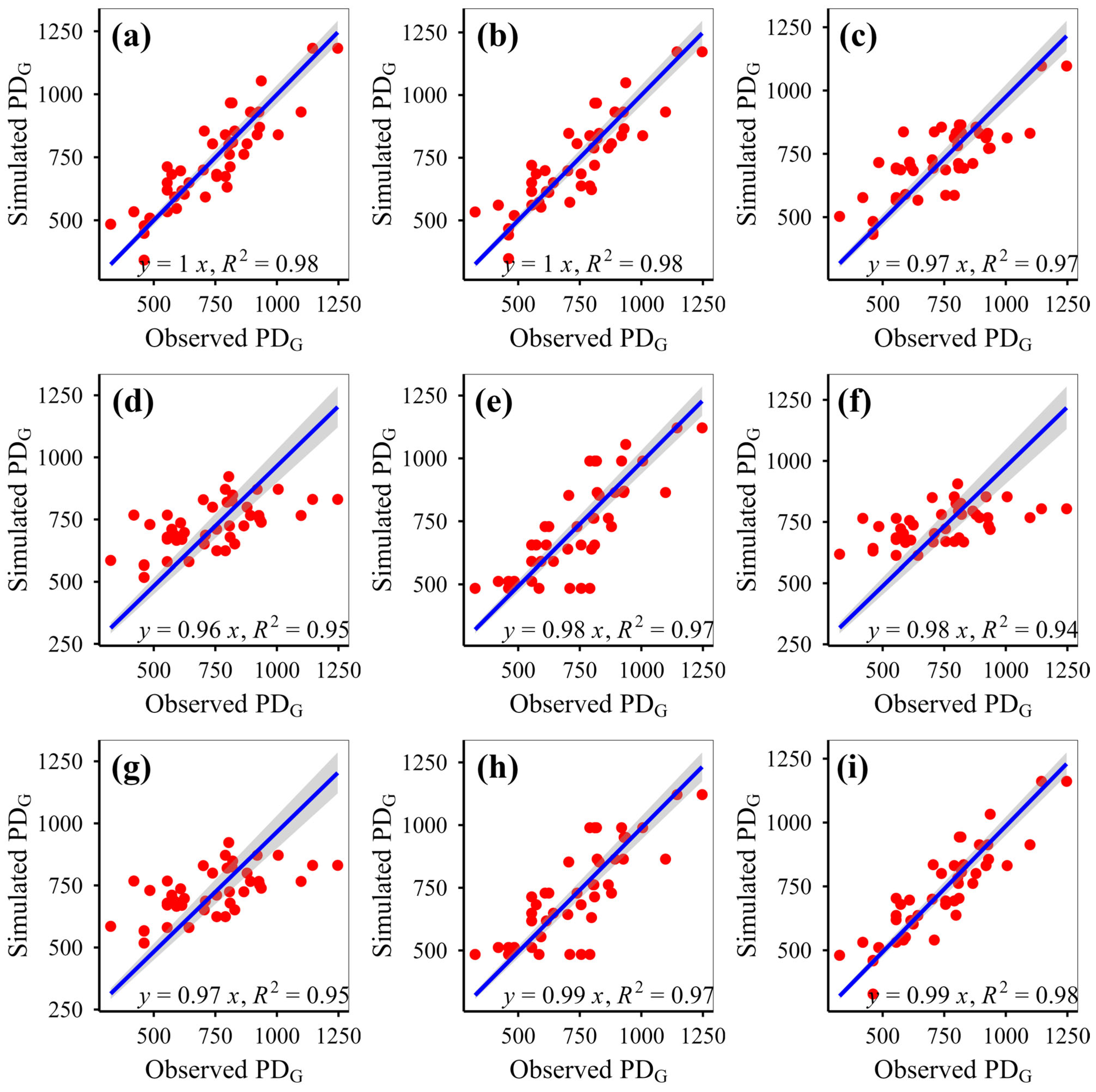
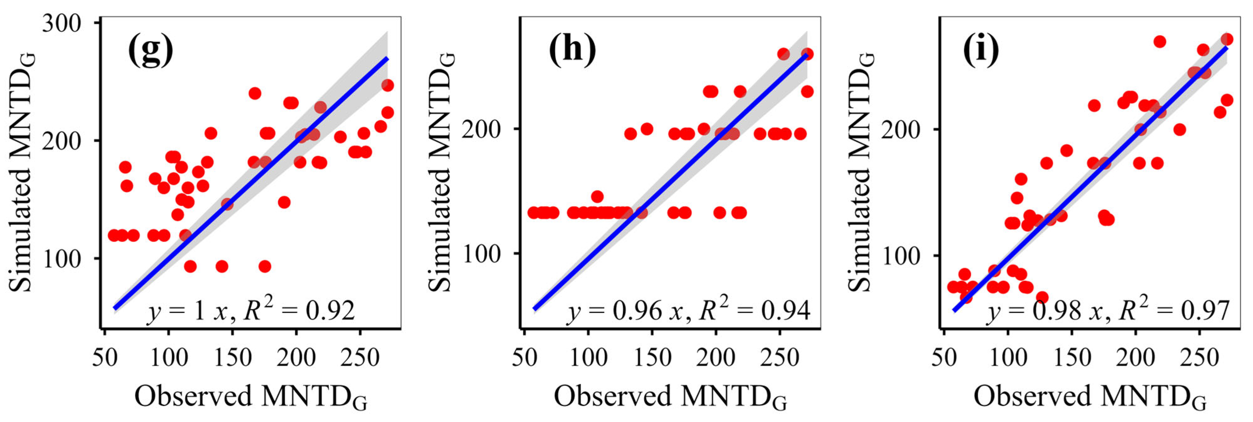
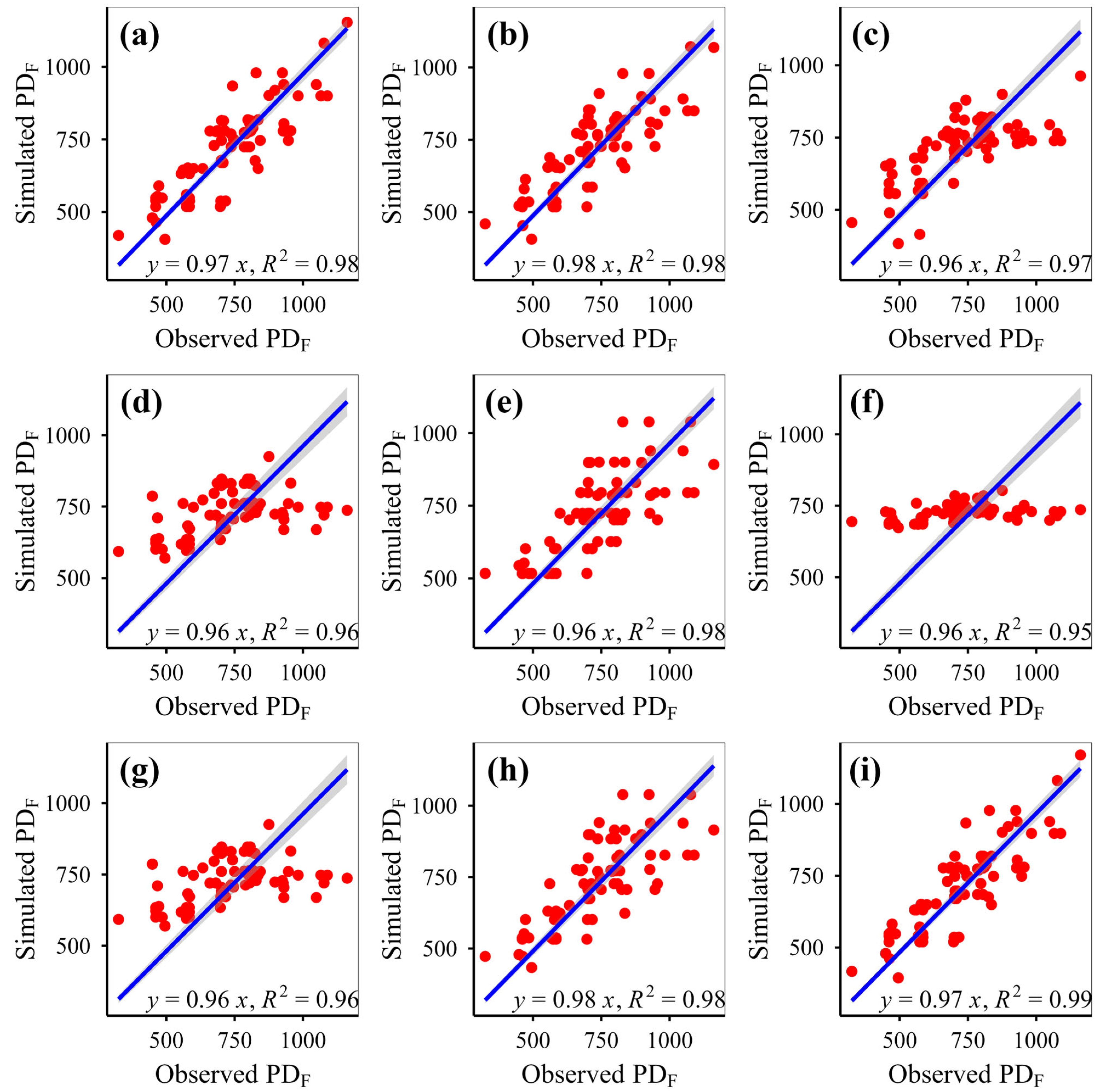
A comparative analysis of nine computational algorithms across 629 observations under fencing and grazing conditions revealed distinct patterns in their predictive accuracy for phylogenetic diversity metrics (Table 1 and Table 2, Figure 1, Figure 2, Figure 3, Figure 4, Figure 5 and Figure 6). The eXGB model achieved the highest precision for specific scenarios: under fencing conditions, it exhibited the lowest relative bias (−0.08%) and RMSE (9.54) for MPD (Figure 2i) and the lowest bias (2.95%) and RMSE (44.86) for MNTD (Figure 3i), while, under grazing conditions, it outperformed other models in predicting PD (bias = 0.33%, RMSE = 29.08). However, eXGB showed limitations for grazing-related MPD and MNTD, where its bias and RMSE were the highest among the top three models (Figure 5i and Figure 6i). In contrast, the RF algorithm demonstrated robust performance, delivering the lowest bias (−1.63%) and RMSE (16.89) for grazing MPD and the lowest bias (−1.09%) and RMSE (27.59) for grazing MNTD (Table 1 and Table 2), alongside competitive accuracy for fencing PD (bias = −1.39%, RMSE = 86.64; Figure 1a). The GBR model exhibited intermediate performance across metrics, exemplified by its bias (4.80%) and RMSE (46.94) for fencing MNTD. Scatterplot analysis (Figure 1, Figure 2, Figure 3, Figure 4, Figure 5 and Figure 6) further validated the exclusion of six models (MLR, RRT, GLR, ANN, CIT, SVM) due to asymmetric distributions or one-to-many value mappings, which undermined their reliability.

4. Discussion

4.1. The Relationship Between Model Structural Differences and Algorithmic Characteristics

Tree-based ensemble methods (RF, GBR) aggregate predictions from multiple base learners, improving robustness through bootstrap aggregation (bagging) or error-correcting boosting algorithms, respectively [24]. In contrast, SVM is kernel function methods based on structural risk minimization, and their complexity mainly lies in the number of support vectors and the dimension of the kernel function [25].
In this study, the model structure parameters (such as the number of trees and the number of support vectors) showed systematic differences under both fenced and grazed conditions, indicating that the model’s sensitivity to data distribution and ecological disturbance responses varies. Firstly, in fencing, tree numbers in the random forest (512–623) lies between GBR (1000 trees) and SVM (280–285 support vectors). This might suggest that RF’s fitting degree is between the overfitting-prone GBR and the more concise SVM. This moderate complexity may be beneficial for dealing with nonlinear and redundant variables in relatively stable ecosystem data (such as fenced plots). Secondly, in grazing, tree numbers in the random forest increased to 723–738, approaching GBR (996–1000), and significantly higher than the number of support vectors in SVM (176–192). Grazing, as an ecological disturbance factor, leads to more complex or unstable data features, thus RF needs to build more decision trees to fully capture the changing features. This is consistent with the existing research viewpoint that RF can better handle high-dimensional non-stationary ecological data [26,27]. The number of support vectors in SVM decreases under grazing conditions, which may indicate that the SVM model has limited adaptability to nonlinear changes in disturbed data or that its kernel function has limited expressive power for such data. SVM typically performs better in scenarios with more regular data structures and less noise [28], which also explains the trend of model structure simplification under grazing conditions.
Therefore, the structural differences among various algorithms reflect their adaptation strategies to the complexity of data and the response mechanisms to ecological disturbances. The increase in model complexity of random forest under grazing conditions indicates its sensitivity and adaptability in capturing nonlinear ecological changes, while the decrease in the number of support vectors in SVM might imply that the model is overly simplified and unable to capture the high heterogeneity of the ecosystem.

4.2. Analysis of the Advantages and Error Characteristics of Ensemble Learning Models in Ecological Prediction

The results of this study demonstrate that RF, as an intrinsic ensemble model, exhibits outstanding simulation capabilities (R2 = 0.66–0.72 and 0.68–0.78, Table A1) in both fenced and grazing management scenarios, significantly outperforming traditional MLR and recursive regression methods (Table A4 and Table A5). This trend validates the robustness and generalization ability of ensemble models in handling nonlinear, multi-dimensional, and high-noise ecological data [24,26].
RF reduces the problem of a single tree being easily influenced by local outliers by voting or averaging the results of multiple decision trees, and it also has robust feature selection capabilities and can automatically handle complex interactions between variables. In this study, RF achieved the highest R2 value in both management scenarios, indicating that it can maintain stable predictive ability under different ecological pressures. This is consistent with the widespread recommendation of RF in ecological modeling for predicting species distribution [27], ecological restoration [29], and other scenarios. In contrast, the R2 values of MLR in both scenarios were relatively low (0.18–0.29), indicating that its linear assumption and sensitivity to multicollinearity limit its application in complex ecosystems [30]. Although recursive regression was slightly better than MLR, it still fell short of RF in terms of variable handling capacity and generalization performance, especially when nonlinearity, interaction, and multiple noises were present.
In terms of training error, eXGB demonstrated the smallest error under the fence conditions (1517.4–8771.17, Table A6), indicating its extremely strong model fitting ability, which is consistent with its algorithm principle of continuously optimizing residuals based on the gradient descent strategy [31]. However, it shows significant fluctuations under grazing conditions, suggesting that it may have a risk of overfitting, especially when the dataset is small or the noise is large [32]. ANN, GLR, and CIT exhibit a certain degree of homogeneity in terms of training error (Table A6), which may stem from their different modeling mechanisms but ultimately share a certain common performance ceiling in ecosystem data modeling. For instance, ANN is prone to becoming stuck in local optima when there are many parameters and limited samples, while GLR is constrained by the linear assumption, and CIT may be overly conservative in data segmentation [29,33].
Overall, RF and eXGB have demonstrated the most superior performance in complex ecological modeling, but the challenges they face (such as RF’s deficiency in interpretability and eXGB’s risk of overfitting) also need to be taken into account. Although ANN, GLR, and CIT have relatively simpler structures, their performance in modeling nonlinear features may be limited. These research results emphasize that, when making ecological predictions such as the phylogenetic diversity of plant communities, the selection of models should comprehensively consider the trade-offs among data characteristics, management scenarios, and algorithm complexity.

4.3. Analysis of the Differences in the Predictive Ability of Algorithms for Phylogenetic Diversity in Plant Communities

This study’s comparative analysis of nine machine learning algorithms under fencing and grazing conditions revealed significant differences in their predictive capabilities for plant community phylogenetic diversity (PD, MPD, MNTD) (Table 1 and Table 2, Figure 1, Figure 2, Figure 3, Figure 4, Figure 5 and Figure 6). The results demonstrate that eXGB and RF, as ensemble learning models, exhibited complementary strengths across different metrics and management contexts, while six other models (MLR, RRT, GLR, ANN, CIT, SVM) were excluded due to unreliable scatterplot distributions (Figure 1, Figure 2, Figure 3, Figure 4, Figure 5 and Figure 6).
Under fencing conditions, the eXGB model achieved exceptional accuracy for fencing scenarios, with the lowest bias (–0.08%) and RMSE (9.54) for MPD (Figure 2i) and optimal performance for MNTD (bias = 2.95%, RMSE = 44.86; Figure 3i). This aligns with its gradient-based iterative optimization mechanism, which excels at capturing stable nonlinear ecological relationships in undisturbed systems [30]. The fencing environment’s reduced background noise (e.g., minimal species turnover) likely enhanced eXGB’s ability to identify key drivers like climate–NDVI interactions [34,35]. In contrast, RF dominated grazing scenarios, delivering the lowest bias (–1.63%) and RMSE (16.89) for MPD, along with robust MNTD predictions (bias = –1.09%, RMSE = 27.59). This reflects RF’s capacity to handle heterogeneous data through its randomized feature selection and multi-tree architecture [24]. Grazing-induced community shifts (e.g., phylogenetic clustering due to herbivory pressure [36]) create non-stationary data patterns where RF’s inherent variance reduction proves advantageous [26].
Notably, eXGB outperformed for grazing PD (bias = 0.33%, RMSE = 29.08), while RF excelled in fencing PD (bias = –1.39%, RMSE = 86.64; Figure 1a). This dichotomy suggests that eXGB’s residual-driven learning is sensitive to perturbation-induced nonlinearities [37], while RF’s bootstrap aggregation stabilizes predictions in structured communities [38]. This aligns with the paradigm that hybrid modeling approaches optimize ecological forecasts [9]. For example, GBR’s intermediate performance (fencing MNTD: bias = 4.80%, RMSE = 46.94) further underscores the value of multi-algorithm benchmarking. Our study advances ecological modeling best practices by demonstrating how integrating condition-specific model selection, multi-metric validation, and algorithmic diversity can systematically address the limitations of single-model approaches in heterogeneous ecosystems. Specifically, our findings advocate for (1) condition-specific model selection—prioritize eXGB for stable systems with clear underlying drivers and RF for disturbed or heterogeneous environments; (2) multi-metric validation—integrate bias and root mean square error (RMSE) with visual scatterplot analysis (Figure 1, Figure 2, Figure 3, Figure 4, Figure 5 and Figure 6) to identify asymmetric prediction patterns; and (3) algorithmic diversity—avoid overreliance on individual models and leverage their complementary strengths, as demonstrated in [39].

5. Conclusions

This study simulated plant phylogenetic diversity under different scenarios (fenced vs. grazed) on the Qinghai-Xizang Plateau using nine models based on various algorithms. This study demonstrates that eXGB, RF, and GBR are the most reliable algorithms for predicting plant community phylogenetic diversity, outperforming the other six models (MLR, RRT, GLR, ANN, CIT, SVM). The eXGB model excels in predicting MPD and MNTD under fencing conditions and PD under grazing conditions, but its accuracy declines for grazing-related distance metrics (MPD/MNTD). In contrast, RF delivers consistent performance, achieving high precision for MPD/MNTD under grazing and PD under fencing, thus offering balanced predictive capability across diverse scenarios. Critically, evaluation of scatterplot integrity (e.g., symmetry along 1:1 lines) and multi-metric validation (bias, RMSE, R2, slope) proves essential for robust model assessment. While no single algorithm dominates all scenarios, eXGB and RF emerge as contextually optimal choices, highlighting the necessity for condition-specific model selection in ecological diversity studies.
Author Contributions

Conceptualization, M.X. and G.F.; methodology, M.X. and G.F.; formal analysis, M.X. and G.F.; data curation, M.X. and G.F.; writing—original draft preparation, M.X., T.M., W.S., S.L. and G.F.; writing—review and editing, M.X., T.M., W.S., S.L. and G.F.; visualization, M.X. and G.F.; funding acquisition, T.M. and G.F. All authors have read and agreed to the published version of the manuscript.

Funding

This research was funded by the Open Project of State Key Laboratory of Plateau Ecology and Agriculture, Qinghai University [2024-ZZ-07], the Lhasa Science and Technology Plan Project [LSKJ202422], the Tibet Autonomous Region Science and Technology Project [XZ202401JD0029, XZ202501ZY0086, XZ202501ZY0056], and Construction of Zhongba County Fixed Observation and Experiment Station of First Support System for Agriculture Green Development.

Data Availability Statement

The data that support the findings of this study are available from the corresponding author upon request.

Conflicts of Interest

The authors declare no conflicts of interest.

Abbreviations

The following abbreviations are used in this manuscript:
RFrandom forest
GBRgeneralized boosted regression
SVMsupport vector machine
MLRmultiple linear regression
RRTrecursive regression tree
ANNartificial neural network
GLRgeneralized linear regression
CITconditional inference tree
eXGBeXtreme gradient boosting
PDFaith’s phylogenetic diversity
MPDmean pairwise distance
MNTDmean nearest taxon distance

Appendix A

Figure A1. Sampling sites.
Diversity 17 00569 g0a1
Table A1. Random forest model parameters of Faith’s phylogenetic diversity (PD), mean pairwise distance (MPD), and mean nearest taxon distance (MNTD) of plant communities under fencing and free-grazing conditions.
ConditionsVariableMean Square ErrorsntreemtryR2n
FencingPD9243.0962330.72323
MPD327.8959420.70323
MNTD1478.4451210.66323
GrazingPD10,773.4973840.78216
MPD367.7772330.71216
MNTD1333.77673240.68216
Table A2. Generalized boosted regression parameters of Faith’s phylogenetic diversity (PD), mean pairwise distance (MPD), and mean nearest taxon distance (MNTD) of plant communities under fencing and free-grazing conditions.
ConditionsVariableTree NosMean Train ErrorMean Cv Errorn
FencingPD100010,886.8617,005.92323
MPD1000373.62495.26 323
MNTD10001501.811945.41323
GrazingPD1000 12,128.3526,462.67 216
MPD1000407.81576.82216
MNTD9961138.531818.57 216
Table A3. Support vector machine parameters of Faith’s phylogenetic diversity (PD), mean pairwise distance (MPD), and mean nearest taxon distance (MNTD) of plant communities under fencing and free-grazing conditions.
ConditionsVariableMean ResidualsMean Decision ValuesSupport Vector Nosn
FencingPD8.09−0.04284323
MPD−4.320.13280323
MNTD0.64−0.01285323
GrazingPD9.25−0.04176216
MPD−3.890.11192216
MNTD−0.3410.01183216
Table A4. Multiple linear regression parameters of Faith’s phylogenetic diversity (PD), mean pairwise distance (MPD), and mean nearest taxon distance (MNTD) of plant communities under fencing and free-grazing conditions.
ConditionsVariableInterceptTemperaturePrecipitationRadiationNDVIR2n
FencingPD−486.52813.760.640.12 0.18323
MPD−271.202.140.130.05 0.19323
MNTD390.801.21−0.23−0.02 0.23323
GrazingPD−1973.5324.390.890.31−159.210.29216
MPD−396.812.890.110.0713.210.22216
MNTD745.88−7.13−0.27−0.06−0.250.35216
Table A5. Recursive regression tree parameters of Faith’s phylogenetic diversity (PD), mean pairwise distance (MPD), and mean nearest taxon distance (MNTD) of plant communities under fencing and free-grazing conditions.
ConditionsVariableR2n
FencingPD0.50323
MPD0.48323
MNTD0.54323
GrazingPD0.73216
MPD0.55216
MNTD0.65216
Table A6. Artificial neural network (ANN), generalized linear regression (GLR), conditional inference tree (CIT), and eXtreme gradient boosting (eXGB) parameters of Faith’s phylogenetic diversity (PD), mean pairwise distance (MPD), and mean nearest taxon distance (MNTD) of plant communities under fencing and free-grazing conditions.
ConditionsVariableANNGLRCITeXGBn
FencingPD14,083.4414,770.0011,918.088771.17323
MPD2721.222822.422025.091517.4323
MNTD5329.865684.374146.593142.62323
GrazingPD10,355.4012,120.759326.096250.41216
MPD1751.641988.911423.661159.05216
MNTD2745.303234.922433.692018.21216

References

  1. Faith, D.P. Conservation evaluation and phylogenetic diversity. Biol. Conserv. 1992, 61, 1–10. [Google Scholar] [CrossRef]
  2. Cadotte, M.W.; Jonathan Davies, T.; Regetz, J.; Kembel, S.W.; Cleland, E.; Oakley, T.H. Phylogenetic diversity metrics for ecological communities: Integrating species richness, abundance and evolutionary history. Ecol. Lett. 2010, 13, 96–105. [Google Scholar] [CrossRef] [PubMed]
  3. Yang, J.; Dong, J.; Xiao, X.; Dai, J.; Wu, C.; Xia, J.; Zhao, G.; Zhao, M.; Li, Z.; Zhang, Y.; et al. Divergent shifts in peak photosynthesis timing of temperate and alpine grasslands in China. Remote Sens. Environ. 2019, 233, 111395. [Google Scholar] [CrossRef]
  4. Cadotte, M.W.; Cavender-Bares, J.; Tilman, D.; Oakley, T.H. Using phylogenetic, functional and trait diversity to understand patterns of plant community productivity. PLoS ONE 2009, 4, e5695. [Google Scholar] [CrossRef] [PubMed]
  5. Qian, H.; Sandel, B. Phylogenetic structure of regional angiosperm assemblages across latitudinal and climatic gradients in North America. Glob. Ecol. Biogeogr. 2017, 26, 1258–1269. [Google Scholar] [CrossRef]
  6. Song, W.; Li, Y.; Luo, A.; Su, X.; Liu, Y.; Luo, Y.; Jiang, K.; Sandanov, D.; Wang, W.; Wang, Z. The Phylogenetic Structure Patterns of Angiosperm Species and Their Determinants in East Eurasia. Glob. Ecol. Biogeogr. 2024, 33, e13897. [Google Scholar] [CrossRef]
  7. Mazel, F.; Mooers, A.O.; Riva, G.V.D.; Pennell, M.W. Conserving phylogenetic diversity can be a poor strategy for conserving functional diversity. Syst. Biol. 2017, 66, 1019–1027. [Google Scholar] [CrossRef]
  8. Thornhill, A.H.; Baldwin, B.G.; Freyman, W.A.; Nosratinia, S.; Kling, M.M.; Morueta-Holme, N.; Madsen, T.P.; Ackerly, D.D.; Mishler, B.D. Spatial phylogenetics of the native California flora. BMC Biol. 2017, 15, 96. [Google Scholar] [CrossRef]
  9. Cadotte, M.W.; Arnillas, C.A.; Livingstone, S.W.; Yasui, S.-L.E. Predicting communities from functional traits. Trends Ecol. Evol. 2015, 30, 510–511. [Google Scholar] [CrossRef]
  10. Chen, Q.C.; Hu, T.; Li, X.H.; Song, C.P.; Zhu, J.K.; Chen, L.Q.; Zhao, Y. Phosphorylation of SWEET sucrose transporters regulates plant root: Shoot ratio under drought. Nat. Plants 2022, 8, 68–77. [Google Scholar] [CrossRef]
  11. Niu, B.; Zhang, X.; Piao, S.; Janssens, I.A.; Fu, G.; He, Y.; Zhang, Y.; Shi, P.; Dai, E.; Yu, C. Warming homogenizes apparent temperature sensitivity of ecosystem respiration. Sci. Adv. 2021, 7, eabc7358. [Google Scholar] [CrossRef]
  12. Ding, J.; Yang, T.; Zhao, Y.; Liu, D.; Wang, X.; Yao, Y.; Peng, S.; Wang, T.; Piao, S. Increasingly important role of atmospheric aridity on Tibetan alpine grasslands. Geophys. Res. Lett. 2018, 45, 2852–2859. [Google Scholar] [CrossRef]
  13. Ran, Q.; Hao, Y.; Xia, A.; Liu, W.; Hu, R.; Cui, X.; Xue, K.; Song, X.; Xu, C.; Ding, B.; et al. Quantitative Assessment of the Impact of Physical and Anthropogenic Factors on Vegetation Spatial-Temporal Variation in Northern Tibet. Remote Sens. 2019, 11, 1183. [Google Scholar] [CrossRef]
  14. Schickhoff, U.; Bobrowski, M.; Mal, S.; Schwab, N.; Singh, R. The world’s mountains in the Anthropocene. In Mountain Landscapes in Transition: Effects of Land Use Climate Change; Springer: Berlin/Heidelberg, Germany, 2022; pp. 1–144. [Google Scholar] [CrossRef]
  15. Khalil, M.I.; Gibson, D.J.; Baer, S.G.; Willand, J.E. Functional diversity is more sensitive to biotic filters than phylogenetic diversity during community assembly. Ecosphere 2018, 9, e02164. [Google Scholar] [CrossRef]
  16. Yang, K.; Jiang, Y.; Tang, W.; He, J.; Shao, C.; Zhou, X.; Lu, H.; Chen, Y.; Li, X.; Shi, J. A High-Resolution Near-Surface Meteorological Forcing Dataset for the Third Pole Region (TPMFD, 1979–2023); National Tibetan Plateau/Third Pole Environment Data Center: Beijing, China, 2023. [Google Scholar] [CrossRef]
  17. R Core Team. A Language and Environment for Statistical Computing. Available online: https://www.R-project.org/ (accessed on 24 April 2024).
  18. Therneau, T.; Atkinson, B.; Ripley, B.; Ripley, M.B. Package ‘rpart’. Available online: https://github.com/bethatkinson/rpart (accessed on 7 January 2025).
  19. Garge, N.R.; Bobashev, G.; Eggleston, B. Random forest methodology for model-based recursive partitioning: The mobForest package for R. BMC Bioinform. 2013, 14, 125. [Google Scholar] [CrossRef] [PubMed]
  20. Greenwell, B.; Boehmke, B.; Cunningham, J.; Developers, G.; Greenwell, B. Package ‘gbm’. Available online: https://github.com/gbm-developers/gbm (accessed on 28 June 2024).
  21. Cortez, P.; Cortez, M.P. Package ‘rminer’. Available online: https://cran.r-project.org/package=rminer (accessed on 4 June 2025).
  22. Meyer, D.; Dimitriadou, E.; Hornik, K.; Weingessel, A.; Leisch, F.; Chang, C.-C.; Lin, C.-C.; Meyer, M.D. Package ‘e1071’. Available online: http://r.meteo.uni.wroc.pl/web/packages/e1071/e1071.pdf (accessed on 16 September 2021).
  23. Zhang, G.; Fu, G. Changes in soil organic carbon, total nitrogen and total phosphorus in 2000–2020 and their driving mechanisms in Tibetan alpine grasslands. Glob. Planet. Chang. 2024, 239, 104484. [Google Scholar] [CrossRef]
  24. Breiman, L. Random Forests. Mach. Learn. 2001, 45, 5–32. [Google Scholar] [CrossRef]
  25. Cortes, C.; Vapnik, V. Support-vector networks. Mach. Learn. 1995, 20, 273–297. [Google Scholar] [CrossRef]
  26. Cutler, D.R.; Edwards, T.C., Jr.; Beard, K.H.; Cutler, A.; Hess, K.T.; Gibson, J.; Lawler, J.J. Random forests for classification in ecology. Ecol. Lett. 2007, 88, 2783–2792. [Google Scholar] [CrossRef]
  27. Elith, J.; Leathwick, J.R.; Hastie, T. A working guide to boosted regression trees. J. Anim. Ecol. 2008, 77, 802–813. [Google Scholar] [CrossRef]
  28. Hsu, C.-W.; Chang, C.-C.; Lin, C.-J. A Practical Guide to Support Vector Classification; National Taiwan University: Taipei, Taiwan, 2003; Available online: http://www.csie.ntu.edu.tw/~cjlin (accessed on 1 May 2025).
  29. Olden, J.D.; Lawler, J.J.; Poff, N.L. Machine learning methods without tears: A primer for ecologists. Q. Rev. Biol. 2008, 83, 171–193. [Google Scholar] [CrossRef] [PubMed]
  30. Dormann, C.F.; Elith, J.; Bacher, S.; Buchmann, C.; Carl, G.; Carré, G.; Marquéz, J.R.G.; Gruber, B.; Lafourcade, B.; Leitão, P.J. Collinearity: A review of methods to deal with it and a simulation study evaluating their performance. Ecography 2013, 36, 27–46. [Google Scholar] [CrossRef]
  31. Chen, T.; Guestrin, C. Xgboost: A scalable tree boosting system. In Proceedings of the 22nd ACM SIGKDD International Conference on Knowledge Discovery and Data Mining, San Francisco, CA, USA, 13–17 August 2016; pp. 785–794. [Google Scholar]
  32. Natekin, A.; Knoll, A. Gradient boosting machines, a tutorial. Front. Neurorobot. 2013, 7, 21. [Google Scholar] [CrossRef] [PubMed]
  33. Ruppert, D. The Elements of Statistical Learning: Data Mining, Inference, and Prediction; Taylor & Francis: Abingdon, UK, 2004. [Google Scholar]
  34. Díaz, S.; Lavorel, S.; de Bello, F.; Quétier, F.; Grigulis, K.; Robson, T.M. Incorporating plant functional diversity effects in ecosystem service assessments. Proc. Natl. Acad. Sci. USA 2007, 104, 20684–20689. [Google Scholar] [CrossRef]
  35. Laliberte, E.; Wells, J.A.; DeClerck, F.; Metcalfe, D.J.; Catterall, C.P.; Queiroz, C.; Aubin, I.; Bonser, S.P.; Ding, Y.; Fraterrigo, J.M. Land-use intensification reduces functional redundancy and response diversity in plant communities. Ecol. Lett. 2010, 13, 76–86. [Google Scholar] [CrossRef]
  36. Weiher, E.; Forbes, S.; Schauwecker, T.; Grace, J.B. Multivariate control of plant species richness and community biomass in blackland prairie. Oikos 2004, 106, 151–157. [Google Scholar] [CrossRef]
  37. Elith, J.; Graham, C.H. Do they? How do they? Why do they differ? On finding reasons for differing performances of species distribution models. Ecography 2009, 32, 66–77. [Google Scholar] [CrossRef]
  38. Buckley, L.B.; Urban, M.C.; Angilletta, M.J.; Crozier, L.G.; Rissler, L.J.; Sears, M.W. Can mechanism inform species’ distribution models? Ecol. Lett. 2010, 13, 1041–1054. [Google Scholar] [CrossRef]
  39. Norberg, A.; Abrego, N.; Blanchet, F.G.; Adler, F.R.; Anderson, B.J.; Anttila, J.; Araújo, M.B.; Dallas, T.; Dunson, D.; Elith, J. A comprehensive evaluation of predictive performance of 33 species distribution models at species and community levels. Ecol. Monogr. 2019, 89, e01370. [Google Scholar] [CrossRef]
Figure 1. Comparison of simulated and observed Faith’s phylogenetic diversity (PD) of plant communities for (a) RF, (b) GBR, (c) SVM, (d) MLR, (e) RRT, (f) GLR, (g) ANN, (h) CIT, and (i) eXGB under fencing conditions. Solid lines show linear regressions between model estimates and field observations. Each red dot represents a single paired observation of observed and simulated values for PD in the samples analyzed.
Diversity 17 00569 g001
Figure 2. Comparison of simulated and observed mean pairwise distance (MPD) of plant communities for (a) RF, (b) GBR, (c) SVM, (d) MLR, (e) RRT, (f) GLR, (g) ANN, (h) CIT, and (i) eXGB under fencing conditions. Solid lines show linear regressions between model estimates and field observations. Each red dot represents a single paired observation of observed and simulated values for MPD in the samples analyzed.
Diversity 17 00569 g002
Figure 3. Comparison of simulated and observed mean nearest taxon distance (MNTD) of plant communities for (a) RF, (b) GBR, (c) SVM, (d) MLR, (e) RRT, (f) GLR, (g) ANN, (h) CIT, and (i) eXGB under fencing conditions. Solid lines show linear regressions between model estimates and field observations. Each red dot represents a single paired observation of observed and simulated values for MNTD in the samples analyzed.
Diversity 17 00569 g003
Figure 4. Comparison of simulated and observed Faith’s phylogenetic diversity (PD) of plant communities for (a) RF, (b) GBR, (c) SVM, (d) MLR, (e) RRT, (f) GLR, (g) ANN, (h) CIT, and (i) eXGB under grazing conditions. Solid lines show linear regressions between model estimates and field observations. Each red dot represents a single paired observation of observed and simulated values for PD in the samples analyzed.
Diversity 17 00569 g004
Figure 5. Comparison of simulated and observed mean pairwise distance (MPD) of plant communities for (a) RF, (b) GBR, (c) SVM, (d) MLR, (e) RRT, (f) GLR, (g) ANN, (h) CIT, and (i) eXGB under grazing conditions. Solid lines show linear regressions between model estimates and field observations. Each red dot represents a single paired observation of observed and simulated values for MPD in the samples analyzed.
Diversity 17 00569 g005aDiversity 17 00569 g005b
Figure 6. Comparison of simulated and observed mean nearest taxon distance (MNTD) of plant communities for (a) RF, (b) GBR, (c) SVM, (d) MLR, (e) RRT, (f) GLR, (g) ANN, (h) CIT, and (i) eXGB under grazing conditions. Solid lines show linear regressions between model estimates and field observations. Each red dot represents a single paired observation of observed and simulated values for MNTD in the samples analyzed.
Diversity 17 00569 g006aDiversity 17 00569 g006b
Table 1. Quantitative assessment of simulation accuracy through relative bias (%) calculations comparing model outputs with field observations for three key phylogenetic metrics: Faith’s phylogenetic diversity (PD), mean pairwise distance (MPD), and mean nearest taxon distance (MNTD) in plant community assemblages.
ConditionsVariableRFGBRSVMMLRRRTGLRANNCITeXGB
FencingPD−1.39−0.85−0.950.40−1.680.620.40−0.17−2.25
MPD0.150.312.68−0.630.21−1.81−0.63−0.24−0.08
MNTD4.224.803.345.524.646.355.513.602.95
GrazingPD1.581.941.062.530.394.442.560.810.33
MPD−1.63−1.48−1.68−3.92−3.81−6.07−3.88−3.76−3.02
MNTD−1.09−0.802.619.123.2411.348.953.16−1.42
Table 2. The RMSE between the simulated and observed Faith’s phylogenetic diversity (PD), mean pairwise distance (MPD), and mean nearest taxon distance (MNTD) of plant communities.
ConditionsVariableRFGBRSVMMLRRRTGLRANNCITeXGB
FencingPD86.6497.34126.02150.10113.91160.60150.10109.6989.92
MPD16.3416.7524.2631.8818.6030.8331.8817.859.54
MNTD45.1746.9454.5662.4449.4363.1262.4450.4544.86
GrazingPD94.65102.34125.07171.84 120.73180.70171.86119.4393.21
MPD16.8917.5023.2131.1921.0636.94 31.1811.4317.81
MNTD27.5928.4541.0550.8233.8954.9650.7442.6329.08
Disclaimer/Publisher’s Note: The statements, opinions and data contained in all publications are solely those of the individual author(s) and contributor(s) and not of MDPI and/or the editor(s). MDPI and/or the editor(s) disclaim responsibility for any injury to people or property resulting from any ideas, methods, instructions or products referred to in the content.