Impact of Climate Change on the Distribution of Cinnamomum malabatrum (Laurales—Lauraceae), a Culturally and Ecologically Important Species of Malabar, Western Ghats, India

Abstract

The impact of climate change on the distribution of Cinnamomum malabatrum (Laurales—Lauraceae), a culturally and ecologically important species in the Malabar region of Western Ghats, India, was studied using a MaxEnt machine learning algorithm. The findings are rooted in extensive field data and advanced modeling techniques. The predicted range shifts and contraction of suitable habitats for the species indicate significant challenges ahead, especially in the Malabar midlands and coastal plains—areas of high endemicity. The proposed conservation strategies provide a comprehensive framework that encompasses the protection of sacred groves, sustainable land-use policies, afforestation, and community conservation strategies within protected areas. This study serves as a clarion call for concerted action and collaboration among researchers, policymakers, local communities, and conservation practitioners to preserve the delicate balance of the ecosystem in the face of environmental change.

1. Introduction

Anthropogenic climate change (CC) is disrupting human and natural systems worldwide, with risks and vulnerabilities projected to increase in the coming decades [1]. There is widespread and mounting evidence implicating CC as the primary reason for global biodiversity loss [2,3]. A meta-analysis of species distribution responses to CC revealed significant decreases (14–28%) from the original biodiversity state for increasing global mean temperatures between 1 °C and 2 °C [4]. Climate change also exacerbates and interacts with other human-induced stressors, such as habitat loss and fragmentation, with biodiverse ecoregions disproportionately impacted [5]. Global efforts such as the Kunming–Montreal Global Biodiversity Framework (signed in December 2022) have set ambitious targets for biodiversity conservation, including protecting at least 30% of the Earth’s surface. In particular, it recommends ‘areas of particular importance for biodiversity’ as needing this protection [6].

The Western Ghats (WG) constitute one such biodiverse tropical–subtropical forest ecoregion in southwestern India. It is of immense global importance due to its dense forest cover, its impact on global climate patterns, such as monsoons, and its impact on biodiversity. The integrity of WG forests has been under threat since the 1850s, a threat that has become pronounced over the past few decades due to human activities. Currently, only 3.2% of the land area of the WG remains intact [7]. Structural degradation and local extinction of rare species have been linked to human impacts in the Nilgiri Biosphere Reserve (NBR) within the WG [8], and the contribution of CC as a threat multiplier to this impact cannot be disregarded. Climate-induced warming has already been attributed to the divergent trends observed in the southwest monsoons over the northern and southern West Ghats (NWG and SWG) in the past 84 years, due to a shift in the low-level jet stream [9]. Previous studies have observed and modeled the effects of CC on several WG species, such as Garcinia indica [10], Piper nigrum [11], Nilgiritragus hylocrius [12], Sholicola albiventris [13], endemic flycatchers Ficedula nigrorufa and Eumyias albicaudatus [14], Herpestes fuscus fuscus [15], Cinnamomum travancoricum [16], Loris lydekkerianus [17], Gyps bengalensis [18], and several sp. of the Myristicaceae family [19], among others.

Cinnamomum malabatrum (Lauraceae) is closely related to C. verum and is commonly confused with Cinnamomum tamala. It is a highly variable endemic species in southern India, particularly in the WG and adjacent regions. Kattu karuva—a locally named aromatic plant identified by Kostermans [20] as Cinnamomum malabatrum—was initially described by Van Rheede [21] in Hortus malabaricus (1685). Kostermans reported that Hooker [22] and Gamble [23] referred to this isotype specimen as Cinnamomum iners. It is also widely reported in the ‘sacred groves’ in the coastal plains of the Alappuzha district (9.14°–9.89° N and 76.26°–76.66° E) in Kerala, which represents one of the indigenous and community-conserved areas recognized by the IUCN [24].

Historically, the unripe fruits of this species have been used as substitutes and adulterants for Cassia buds. They are also used as clove bud substitutes in ‘paan’, a widespread chewing habit in South Asia. Although its bark is inferior to true cinnamon, aromatic leaves are vital to many culinary traditions and indigenous medical practices. The bark is marketed as a nontimber forest product (NTFP) by the indigenous Kattunaikka tribe in the Wayanad Wildlife Sanctuary, Kerala [25]. Phytochemical studies on its leaves have revealed its anticancer, antimicrobial, and anti-inflammatory properties [26]. Its essential oil was also shown to have inhibitory effects on enzymes involved in diabetes [27]. Additionally, certain phytoconstituents found in leaf extracts are being explored as potential innovative drug candidates for addressing and managing hyperandrogenism associated with polycystic ovary syndrome (PCOS) [28]. The bark and its infusion are used to treat coughs, colds, toothaches, liver complaints, gallstones, and serve as a mouth freshener [27]. In ayurvedic practice, the dry, unripe fruit of C. malabatrum has been used as ‘Nagakesar’, a substitute for the dried buds of Mesua ferrea [27]. More recently, the bark of C. malabatrum has been dried, powdered, and utilized as a base material for incense sticks known as “agarbathi” in vernacular languages. The leaves are employed as a holding substratum for steaming during the preparation of certain dishes, known locally as ‘thirali’ or ‘elayappam’ [27]. The wood is also valued as high-quality fuel [29].

This species plays a vital role in the forest-associated economies of WG states and could lead to the development of novel pharmacological products. The population of this species has significantly declined due to indiscriminate felling, raising serious conservation concerns [27,30]. Despite its ecological and socioeconomic importance, the impact of CC on the habitat and range of the Cinnamomum genus remains understudied in India. Research on endemic Cinnamomum species from WG has focused on characteristics such as essential oil composition [29]; therefore, species from the Cinnamomum genus have received increased attention in other parts of the world. Research from China on C. mairei and C. camphora has revealed range shifts in the northeast and northwest, respectively, accompanied by slight range expansions [31,32]. However, research from Australia revealed a decline of up to 99% for C. propinquum in 2080 [33]. Research and conservation efforts within the genus could be influenced by a “charisma bias”, where better-known species, such as true Cinnamon (C. verum) and camphor (C. camphora), receive more attention. With this in mind, we contend that this understudied, culturally important, and pharmacologically valuable species warrants proactive research to plan for its conservation. Studying the impact of CC on the vulnerability of C. malabatrum is crucial, given the limited comprehensive research on its susceptibility to climatic shifts. However, few investigations on anthropogenic threats have been conducted [27,30].

This study provides the first spatially explicit assessment of C. malabatrum’s fundamental climate niche and projected range dynamics, aiming to establish a foundational understanding of its ecological requirements in the context of climate change. We ask: What is the potential (fundamental) extent of suitable habitat for this species under current and future climatic conditions, and what do these patterns suggest about its long-term vulnerability and conservation prospects? We hypothesize that C. malabatrum, as a mid-elevation endemic, may exhibit elevation-dependent contraction and possible southward shifts under drying trends projected for the WG, particularly in the dry season. These dynamics have been observed in other montane endemics that are subject to climatic filtering and have limited upslope refugia [34,35]. To examine this, we use MaxEnt to model the species’ fundamental niche under three IPCC AR6 Shared Socioeconomic Pathways (SSP1-2.6, SSP3-7.0, and SSP5-8.5) for the years 2040, 2070, and 2100. Our specific objectives are as follows: (1) to model current and projected distributions of C. malabatrum; (2) to quantify changes in suitable habitat and identify areas of potential range contraction or expansion; and (3) to evaluate the species’ ecological niche based on a broad set of environmental predictors, which has been shown to improve model performance [36,37]. As previous studies have mainly focused on phytochemical traits, this work fills a critical gap by offering a spatially grounded perspective on an ecologically, culturally, and pharmacologically important species. By situating our analysis within a biodiversity hotspot experiencing both climatic and anthropogenic pressures, we aim to inform conservation planning, including reserve expansion and climate-integrated management strategies.

2. Materials and Methods

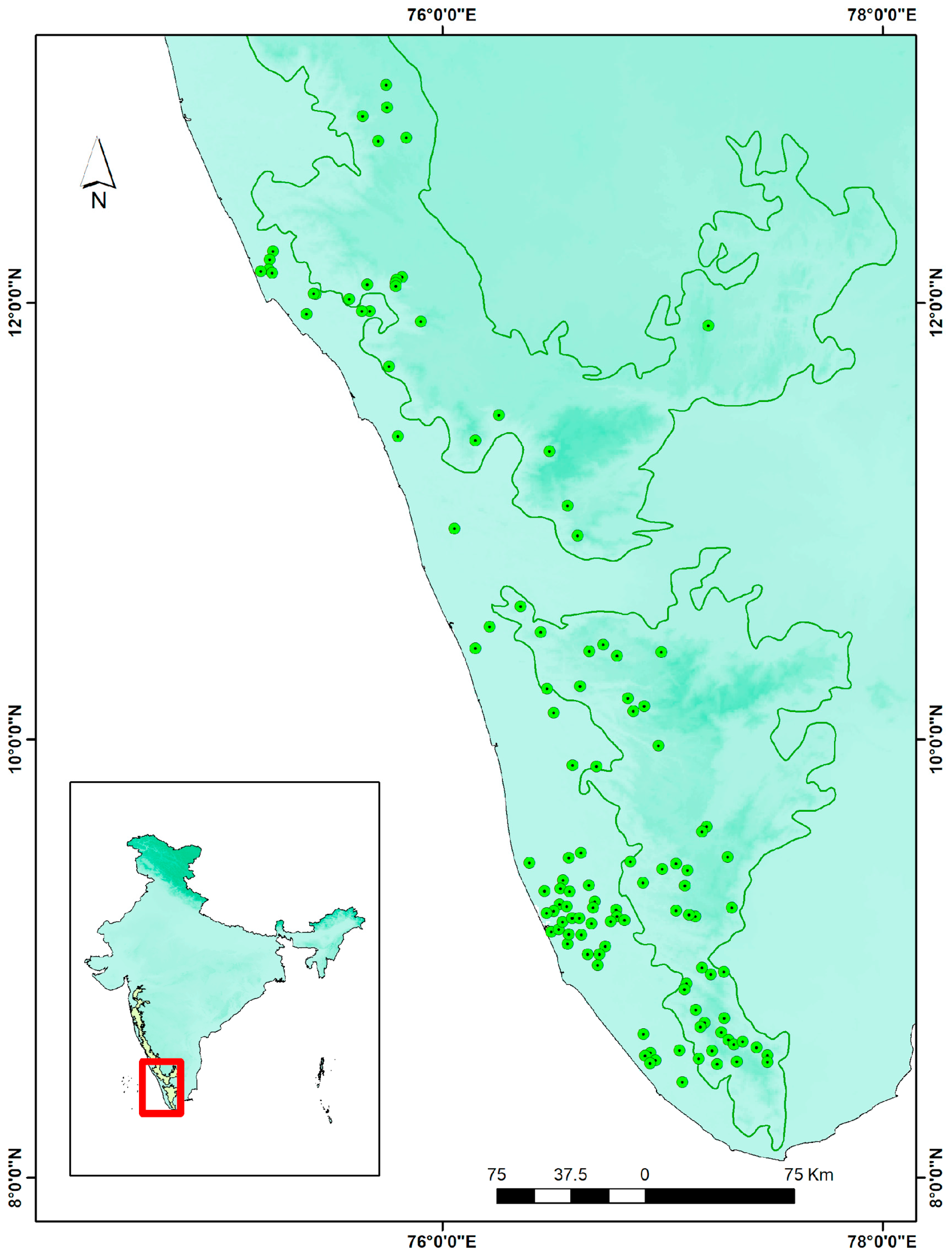
2.1. Study Area

The present study is focused on southwestern India, with a primary emphasis on the states of Kerala (8.29–12.76° N and 74.86–77.28° E) and Karnataka (11.59–18.45° N and 74.09–78.58° E). Our investigation focuses on the distribution of C. malabatrum within the WG, an extensive mountain range (8°–21° N and 73°–89° E) that stretches ~1600 km along the Malabar and Konkan coasts of peninsular India and is spread across Tamil Nadu, Kerala, Karnataka, Goa, Maharashtra, and Gujarat. This region is celebrated for its remarkable biodiversity and endemism, encompassing several distinctive hotspots [38], including Mahabaleshwar (17.92° N, 73.64° E), Palani Hills (10.21° N, 77.39° E), Nilgiris (11.37° N, 76.76° E), Anamalai (10.3° N, 77° E), Silent Valley (11.07° N, 76.43° E), and Agasthyamalai (8.13°–9.17° N, 76.87°–77.57° E). Notably, Nilgiri and Agasthyamalai have received the Biosphere Reserve status, with Nilgiri additionally holding the prestigious UNESCO World Heritage Site designation. The Nilgiri and Anamalai regions in the WG mountain range include peaks rising over 2500 m above sea level (asl). The WG is interrupted by three gaps—south to north—the Shencottah–Achankovil gap (8–9° N, 77–78° E), a major 30–40 km wide Palghat gap (10–11° N, 76–77° E), and the Goa gap (14–15° N, 74–75° E).

The study area explicitly encompasses the SWG, one of the four ecoregions within the WG. The WG ecoregions include the moist deciduous forests and montane rainforests of NWG and SWG, respectively. We restricted our study to areas within SWGs, the adjacent midlands, and coastal plains, where the highest occurrence points for C. malabatrum were identified in existing records. While some records exist for outlier points in interior Tamil Nadu, southern Karnataka, and Goa, these records have been excluded to concentrate our efforts on the region where conservation initiatives can have the most significant impact. Our study area encompasses 25 districts, with 14 in Kerala, 5 in Karnataka, and 6 in Tamil Nadu (see

Table 1. Districts where Cinnamomum malabatrum is found (the % area in columns 3 and 4 was calculated by the authors using raster operations in QGIS 3.16 Hannover software).

State	District Name	% Area of District Suitable for C. malabatrum	% of the Total Suitable Area of C. malabatrum Present in the District
Karnataka	Chikmagalur	1.59%	0.47%
	Dakshin Kannad	1.83%	0.35%
	Hassan	1.18%	0.33%
	Kodagu	20.29%	3.44%
	Udupi	0.13%	0.02%
Kerala	Alappuzha	91.86%	4.73%
	Ernakulam	58.19%	5.42%
	Idukki	60.26%	12.44%
	Kannur	65.31%	7.49%
	Kasaragod	6.57%	0.53%
	Kollam	98.14%	9.76%
	Kottayam	81.75%	7.11%
	Kozhikode	43.45%	4.08%
	Malappuram	17.05%	2.47%
	Palakkad	17.98%	3.33%
	Pathanamthitta	96.90%	10.56%
	Thiruvananthapuram	91.54%	7.73%
	Thrissur	32.88%	4.00%
	Wayanad	41.83%	3.67%
Tamil Nadu	Coimbatore	6.36%	1.95%
	Dindigul	2.67%	0.67%
	Kanniyakumari	35.45%	2.33%
	Nilgiris	16.79%	1.77%
	Theni	5.66%	0.67%
	Tirunelveli	16.68%	4.67%

). Please note that the district names in the table below have been populated based on the modeled current habitat suitability and not the occurrence dataset. As such, there may be some mismatches—for example, Dakshin Kannada, Udupi, and Dindigul, which do not feature in our occurrence records but, upon modeling, are shown to have minuscule areas of the total suitable area of the species—0.35%, 0.02%, and 0.67%, respectively.

In addition to the WG, C. malabatrum is also found in the neighboring Malabar Coast (8–12° N, 75–77° E), which is characterized by the Malabar moist forest, a subtype of tropical evergreen forest. This region is notable for its high population density and extensive forests, primarily in designated protected areas. However, scattered pockets of native vegetation persist, primarily due to the settlement patterns of individual households, which often feature home gardens. The region experiences an annual temperature range of 22–32 °C and receives an average annual precipitation of approximately 3000 mm [39].

2.2. Species Occurrence and Collection of Field Data

For this study, we collated species occurrence records from two key sources: the Indian Biodiversity Information Portal (https://indiabiodiversity.org/) and the Global Biodiversity Information Facility database (https://www.gbif.org/). To enrich our dataset, we also incorporated select data points from field visits, the literature, published CD–ROMs [40], citizen science records [41], and herbarium records [42]. In addition, geolocation details from various published studies and scientific databases, such as the Atlas of endemics of the Western Ghats, India (AEWG), include the distribution of tree species in evergreen and semi–evergreen forests, following Pascal and Ramesh [40], which resulted in a comprehensive dataset comprising 122 records (see

Table 2. Occurrence points and endemicity of Cinnamomum malabatrum used for computational modeling after spatial thinning.

Species Name	Endemic/Non-Endemic	Prevalence Localities	Occurrence (Spatial Thin x = 10 km)
Cinnamomum malabatrum	Endemic to SWG	122	56

). All records span an elevation gradient from 98 m to 1745 m above sea level, with a median of 694 m. Supplementary Table S1 provides the latitude and longitude records, the name of the location, and the district for each point. The modeling relies on aggregated data sources for spatial and temporal coverage, utilizing data from citizen science contributions such as GBIF, Pl@ntNet, and iNaturalist. Detailed systematic sampling techniques are documented in the AEWG database by Pascal and Ramesh [40].

To ensure data accuracy, all data locations were standardized to the WGS84 datum using ArcGIS 10.4 software. Figure 1 maps all the occurrence points included in our primary dataset.

2.3. Elimination of Sampling Biases via Spatial Thinning

Ensuring the accuracy and reliability of model predictions hinges on effectively eliminating or reducing sampling bias. Sampling bias can be introduced through various sources, including uneven sampling efforts across regions or habitats, a preference for easily accessible areas, a bias toward regions with relatively high human population density or research activity, and the absence of some species in online databases, resulting in an incomplete representation of species distribution.

One commonly employed strategy to mitigate sampling bias and enhance model accuracy is ‘spatial thinning’. This approach accounts for bias in favor of well-surveyed regions while concurrently diminishing spatial autocorrelation and overfitting, as described by Kramer-Schadt et al. [43]. In datasets with a relatively substantial number of occurrence records, spatial thinning proves advantageous over ‘background manipulation’, which involves modifying environmental data to mirror the same bias in occurrence data.

In this study, spatial thinning was deployed to reduce the number of occurrence points from 110 to 56 (see Table 2). This was accomplished by retaining only one record within a 10 km radius. We utilized the ‘spThin version 0.2.0’ package in R Studio 1.4.1717, employing the nearest neighbor distance (NND) to enhance the accuracy and reliability of our model predictions.

2.4. Occurrence Data and the Fundamental Niche

The Special Distribution Model (SDM) incorporates occurrence records from aggregated data sources that span both historical and contemporary periods. There has been a significant land-use change and other anthropogenic pressures within the study region. Consequently, some of the records used may reflect areas that no longer support viable populations of C. malabatrum. However, our modeling objective is to approximate the species’ fundamental niche, i.e., the full range of environmental conditions under which it is known to persist, rather than its currently occupied realized niche [44]. The realized niche is restricted by dispersal limitation, interspecific competition, and, crucially, land-use change. However, the fundamental niche remains a more accurate representation of a species’ potential persistence under environmental conditions [45]. This approach aligns with ecological theory, indicating that the realized niche is often a constrained subset of the fundamental niche due to biotic interactions and anthropogenic alterations [46,47]. Given that C. malabatrum remains poorly studied within its genus, reliance solely on recent or confirmed presences would risk underrepresenting its ecological breadth. Faurby and Araújo [48] demonstrate that excluding occurrence records from regions experiencing anthropogenic range contractions can lead to a systematic underestimation of environmental suitability, resulting in biased projections under CC scenarios. The rationale is also supported by Jarvie and Svenning [49], who argue that eliminating occurrences based on current land-use can truncate the realized niche, resulting in spatial bias in correlative models. By incorporating all available occurrence data (subject to spatial thinning to minimize sampling bias), we aim to develop a more robust characterization of the species’ fundamental niche, which is crucial for evaluating future range dynamics under changing climatic conditions.

2.5. Environmental Variables

We employed a comprehensive set of 54 abiotic environmental variables as predictors of species distribution. This dataset comprises 19 bioclimatic variables, which are considered more meaningful than using absolute temperature and precipitation values in establishing relationships between species distributions and climatic factors. These bioclimatic variables encompass parameters such as the maximum temperature of the warmest month and the precipitation of the driest month. Additionally, these variables included other variables of ecological importance, such as the Koppen climate classification, potential evapotranspiration rate, soil attributes, and vegetation indices, collectively contributing to the comprehensiveness of our predictive model. See

Table 3. Environmental variables considered as predictors of species distribution for C. malabatrum prior to a multicollinearity check.

Variable Name	Expansion
bio1	Mean annual air temperature
bio2	Mean diurnal air temperature range
bio3	Isothermality
bio4	Temperature seasonality
bio5	Mean daily maximum air temperature of the warmest month
bio6	Mean daily minimum air temperature of the coldest month
bio7	Annual range of air temperature
bio8	Mean daily mean air temperatures of the wettest quarter
bio9	Mean daily mean air temperatures of the driest quarter
bio10	Mean daily mean air temperatures of the warmest quarter
bio11	Mean daily mean air temperatures of the coldest quarter
bio12	Annual precipitation amount
bio13	The precipitation amount of the wettest month
bio14	The precipitation amount of the driest month
bio15	Precipitation seasonality
bio16	Mean monthly precipitation amount of the wettest quarter
bio17	Mean monthly precipitation amount of the driest quarter
bio18	Mean monthly precipitation amount of the warmest quarter
bio19	Mean monthly precipitation amount of the coldest quarter
soil	Categorical soil map
aspect	Compass direction of the slope of the terrain
ndvi	Normalized difference vegetation index
drainage	Drainage map of the terrain
alt	Altitude
waterbody	Categorical map of waterbodies
aridity	Aridity index
slope	Slope of terrain
pet	Annual potential evapotranspiration
pet_1	Monthly potential evapotranspiration—January
pet_2	Monthly potential evapotranspiration—February
pet_3	Monthly potential evapotranspiration—March
pet_4	Monthly potential evapotranspiration—April
pet_5	Monthly potential evapotranspiration—May
pet_6	Monthly potential evapotranspiration—June
pet_7	Monthly potential evapotranspiration—July
pet_8	Monthly potential evapotranspiration—August
pet_9	Monthly potential evapotranspiration—September
pet_10	Monthly potential evapotranspiration—October
pet_11	Monthly potential evapotranspiration—November
pet_12	Monthly potential evapotranspiration—December
npp	Net Primary productivity
landcover	Categorical map of land cover
gst	Mean temperature of the growing season
gsp	Accumulated precipitation amount on growing season days
gsl	Growing season length
gdd0	Growing degree days heat sum above 0 °C
gdd5	Growing degree days heat sum above 5 °C
gdd10	Growing degree days heat sum above 10 °C
kg0	Köppen–Geiger climate classification
kg1	Köppen–Geiger climate classification without As/Aw distinction
kg2	Köppen–Geiger climate classification [45]
kg3	Köppen–Geiger climate classification [50]
kg4	Köppen–Geiger climate classification [51]
kg5	Köppen–Geiger climate classification [52]

for the complete list of environmental variables.

Forty-five of the 54 variables we used were obtained from the CHELSA (Climatologies at High Resolution for the Earth’s Land Surface Areas) project [53]. From the CHELSA-BIOCLIM+ dataset [53], data were preprocessed in the following manner—data for the present day were obtained by averaging yearly data from 1981 to 2010, and those for 2040, 2070, and 2100 were obtained by averaging annual data from 2011 to 2040, 2041–2070, and 2071–2100, respectively.

Apart from bioclimatic variables, we relied on specific variables such as ‘Landcover’ and ‘NDVI’, which were derived from satellite imagery acquired from BHUVAN, a geospatial platform developed by the Indian Space Research Organization (ISRO). Specifically, we accessed the 1:10,000 scale map and subsequently resampled it using the “resampling” SDMtoolbox v2.6 in ArcGIS 10.4. We meticulously prepared the data via QGIS 3.16 Hannover tools for variables not sourced from external databases. Moreover, variables such as “aspect”, “slope”, “drainage”, and “waterbody” were constructed using ArcGIS 10.4, with data originating from digital elevation model (DEM) maps downloaded from the Databasin portal [54]. The ‘soil’ variable was extracted from a map available in the Food and Agriculture Organization (FAO) database [55], initially at a 10 km × 10 km resolution, and subsequently resampled and upscaled to a 1 km × 1 km raster, which is consistent with the resolutions of the other datasets.

To ensure consistency across future scenarios, we retained constant values for nine variables: land cover, aridity, NDVI, aspect, slope, drainage, water body, altitude, and soil. Although dynamic land-use datasets such as the global 1 km plant functional type projections [56] now exist, at the time of model construction, these were either not yet widely integrated into high-resolution SDM workflows or lacked compatibility with the CHELSA climate layers used in our framework. As noted in Section 2.4 above, our objective here was to estimate the species’ fundamental niche rather than the realized niche shaped by present-day land-use. Moreover, in our final model, land cover and NDVI contributed minimally to predictive performance (permutation importance < 2%), further justifying their static treatment (see Section 3.1 below). While recent studies [57,58] have demonstrated the utility of integrating land-use transitions into SDMs, they also highlight substantial uncertainty and difficulty in aligning such projections with species-level modeling at landscape scales. We have therefore opted for a methodologically stable, climate-driven framework, but acknowledge that future model iterations may benefit from the inclusion of SSP-aligned land-use layers as integration tools mature.

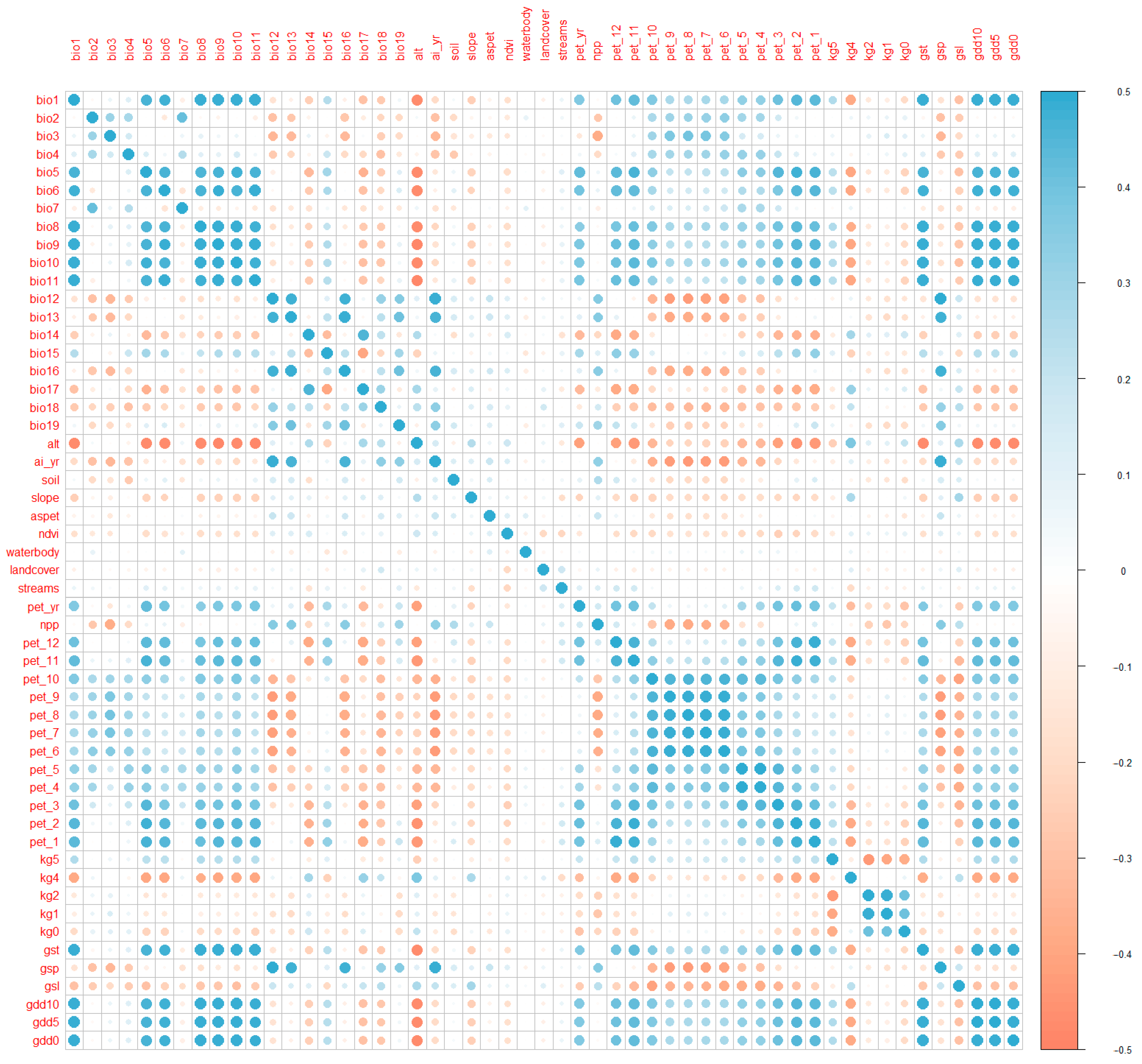
2.6. Multicollinearity

Multicollinearity, characterized by linear relationships among predictor variables in a statistical model, can lead to erroneous inferences of species distributions and, subsequently, the development of inaccurate distribution models [59]. To mitigate multicollinearity-related inaccuracies, we conducted a thorough examination of the pairwise Pearson correlation coefficients among our 54 predictor variables, following the approach of Mateo et al. [60]. Variables exhibiting a high correlation with |r| > 0.8 were removed. In some instances, the threshold for removal was set higher, such as |r| > 0.85 [61,62]. The dataset was refined after collinear variables were eliminated, leaving us with 20 variables for further analysis. See Figure 2 for an illustration of multicollinearity between variables.

2.7. Shared Socioeconomic Pathways

Shared Socioeconomic Pathways (SSP) are scenarios identified by the Intergovernmental Panel on Climate Change (IPCC), which characterize and describe developmental ‘pathways’ for global society based on the absence or extent of climate policies [63]. Among the scenarios and forecasts focused on CC, the SSP largely supplanted RCP (Regional Concentration Pathways) because the SSP provides a more comprehensive framework. Five different SSPs exist, which have varying challenges in either the mitigation or adaptation space [64]. The Model Intercomparison Project (MIP) for CMIP–6 identified multiple projected scenarios (Tier 1, or baseline) to be modeled among all possibilities [65]. The present study utilizes three of these scenarios, along with their corresponding radiative forcing levels—SSP1—2.6, SSP3—7.0, and SSP5—8.5—during three future periods: 2040, 2070, and 2100—to develop a species distribution model (SDM) for C. malabatrum. The three pathways represent distinct trajectories: SSP1 denotes a sustainable or optimistic pathway; SSP3 represents a middle-of-the-road pathway; and SSP5 corresponds to a highly pessimistic pathway, facilitating clearer and more interpretable results.

We used CMIP–6 models over CMIP–5 because the former is reported to show ‘significant improvement’ over CMIP–5 in ‘capturing the spatio–temporal pattern of monsoon over Indian landmass, especially in the WG’, and they capture monsoon onset and extreme events better, two parameters with ecological significance. The improvement in capturing WG precipitation is because the CMIP–5 global circulation model (GCM) with coarser resolution does not accurately capture orographic precipitation, a limitation noted in previous SDM efforts in WG [66].

We used a downscaled, high–resolution dataset with a grid size of ≊30 arc-seconds (≊1 sq. km) provided by the CHELSA project. CHELSA Version–2.1 [67,68] provides data from five GCMs, of which (1) Geophysical Fluid Dynamics Laboratory Earth System Model Version 4 (GFDL ESM–4) [69] and (2) Meteorological Research Institute Earth System Model Version–2 (MRI ESM–2) were used for our research, following Yukimoto et al. [70]. The average of these two models is relevant to the Indian climate scenario [71,72].

Although our choice of GFDL-ESM4 and MRI-ESM2-0 was informed by their demonstrated performance in capturing WG precipitation patterns, we acknowledge that restricting to two GCMs may limit the representation of inter-model uncertainty. A broader ensemble of CMIP–6 models could offer a more comprehensive range of possible futures, particularly for sensitive variables such as dry-season precipitation. However, this must be weighed against the potential for increased projection noise and ecological misalignment at local scales.

2.8. MaxEnt Modeling

Species distribution models (SDMs) are empirical or mathematical models that correlate species occurrence data with environmental and geographical conditions to predict suitable habitat ranges [73]. They require geographically referenced occurrence data and ecologically relevant variables to generate spatial maps of species suitability as outputs. Among various SDM techniques, MaxEnt (maximum entropy) has demonstrated notable advantages, including its ability to handle presence–only data and small sample sizes efficiently, and is the most preferred computational tool when dealing with species with low numbers of reported sightings [74,75].

In a comparative analysis of 12 algorithms, MaxEnt exhibited superior predictive capability with small sample sizes and ranked among the top performers across all sample sizes [76]. MaxEnt has been benchmarked against other SDMs (e.g., BRT, GLM, GAM) in comparative studies and found to perform well in data-scarce settings [77]. MaxEnt operates by integrating environmental variables in .asc files with occurrence records in .csv files. We used the maximum entropy model (Maxent version 3.3.3) [78] to map the past, current, and future distributions of C. malabatrum.

Numerous studies conducted in recent years have suggested that the MaxEnt model’s default settings, which are primarily based on empirical adjustments, may result in suboptimal model performance [79,80]. This study optimized the choice of original predictor variables, also known as “feature classes” or FC, by expanding the combination of feature classes to enhance the model’s flexibility and fitting ability, resulting in improved predictive capability. In particular, 56 C. malabatrum distribution records were split into a 3:7 proportion, with 70% allocated for training and 30% for testing. Furthermore, six feature class (FC) parameter combinations (including L, LQ, H, LQH, LQHP), and 13 regularization multiplier (RM) parameters. LQHPT was established, where L stands for linear, Q for quadratic, H for hinge, P for product, and T for threshold. The 78 parameter combinations mentioned above were tested using the ENMeval 2.0.5 package in R Studio 1.4.1717 software, and the model’s fit and complexity were assessed using the Akaike Information Criterion corrected (AICc), to obtain the combination of parameters with the lowest delta value. The best model was ultimately determined by the AICc value. Following optimization, feature class LQ (linear + quadratic) with an RM (rm = 1) was the final parameter combination found. To verify the stability and dependability of the model, as mentioned, 30% of the data was used as the test set, and the runs were repeated 15 times to ensure robust predictions.

The settings and variables used for model building significantly affect MaxEnt’s performance [81]. We employed the ‘ENMeval 2.0.5’ package following Muscarella et al. [82] to refine our model. ENMeval 2.0.5 suggests initial models and settings, such as the regularization multiplier and the number of background points. We selected the model with the lowest Akaike information criterion (AIC) value. The variables with the lowest contribution and permutation importance were excluded, and the ENMeval 2.0.5 tool was rerun using the remaining variables, iterating until a model with the lowest AIC value was obtained.

The final MaxEnt model was run with 10–fold cross-validation, using 10,000 background points and 5000 iterations. The output format was set to ‘complementary log-log’ (cloglog), which is most suitable for estimating the probability of species presence [78]. The permutation importance percentage and jackknife test gain values of the variables provided insights into the significance of the predictor variables in determining species suitability.

2.9. Justification for Variable-to-Occurrence Ratio in MaxEnt Modeling

While our final model employed 20 environmental predictors with only 56 presence records (post-spatial thinning), we addressed potential overfitting through rigorous multicollinearity filtering, permutation importance, and jackknife testing. Although the variable-to-sample ratio may seem high, studies suggest that in small-sample contexts, effective regularization and careful variable selection are more critical than strict thresholds [83]. We applied MaxEnt’s automatic feature selection with a regularization multiplier of 2, enabling the adaptive incorporation of hinge features, which are suited for small datasets [79]. While ENMeval-based tuning using AICc is valuable, its complexity may be less suited to data-limited and narrow-range species such as C. malabatrum. Recent work [84,85] supports the use of hinge features in such contexts, as they strike a balance between flexibility and ecological realism. Therefore, our modeling strategy reflects best practices for small-sample SDMs by integrating variable pruning, moderate regularization, and interpretable feature use to ensure robust predictions under presence-only constraints.

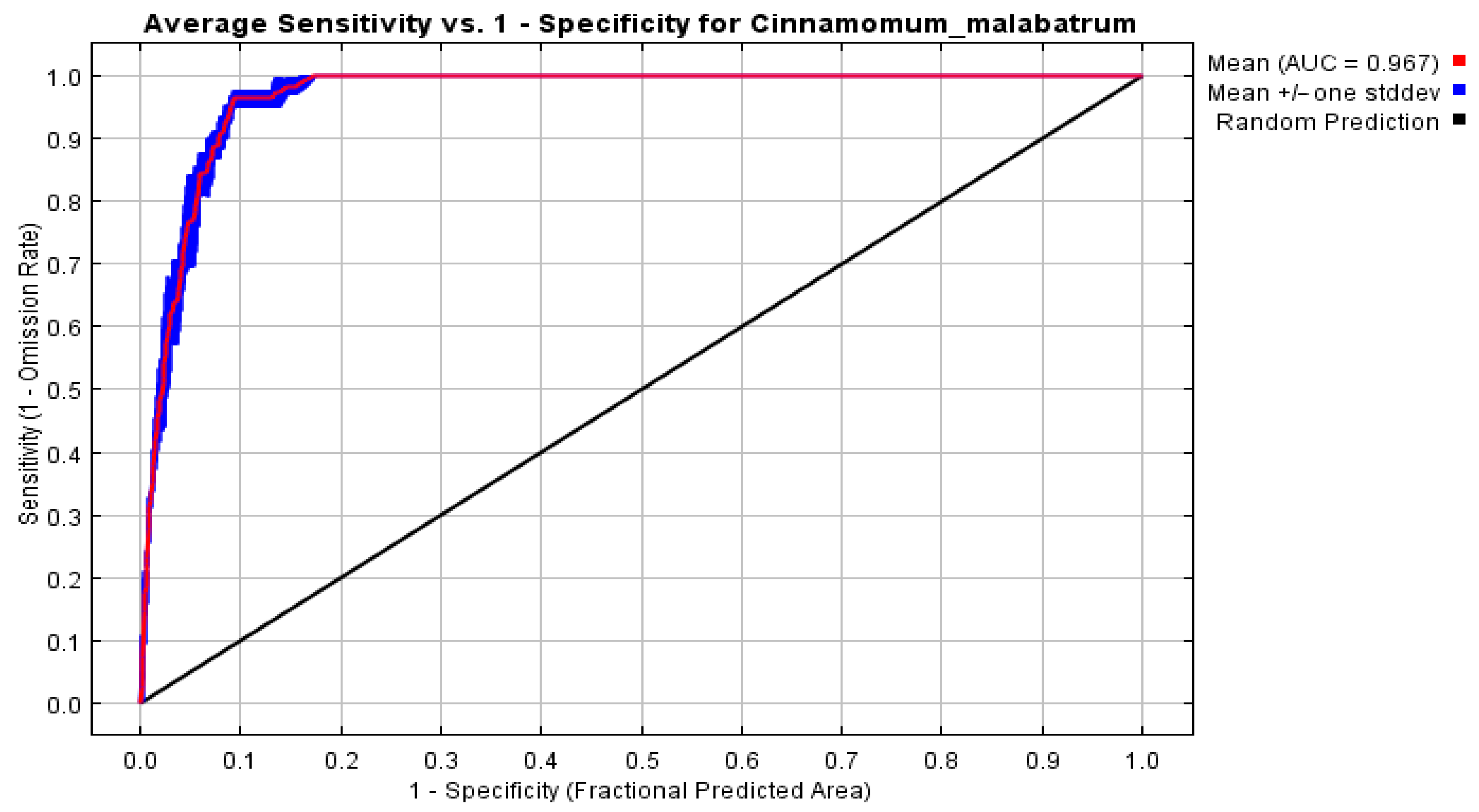
2.10. Model Validation

Model validation is crucial to ensure that the model accurately reflects the patterns and relationships in the data and can be successfully generalized to new data. A validated model also ensures that it outperforms random guessing and minimizes the risk of overfitting, which occurs when the model fits the training data too closely and performs poorly on new data. Species distribution models based on MaxEnt use several validation techniques, and it is often necessary to use a combination of techniques to ensure accuracy. We used four methods: (1) true skill statistics (TSSs); (2) kappa; (3) receiver operating characteristic (ROC)/area under the curve (AUC); and (4) jackknife tests.

The TSS and kappa coefficients are measures of agreement between the model’s predictions and the observed data, taking into account possible omissions (false negatives and false positives). However, while the kappa coefficient is influenced by prevalence, the TSS coefficient is not. The dependence of kappa on prevalence has been claimed to introduce “bias and statistical artifacts into estimates of accuracy,” a shortcoming not shared by TSS, because it is independent of prevalence [86]. Both can have values ranging between −1 and +1, with a value of 0 indicating that the model performs no better than a random guess. Values closer to 1 indicate better model validity [86]. Over three runs, our model achieved averages of 0.70 for the kappa coefficient and 0.85 for the TSS (see

Table 4. Model validation using additional independent statistics such as the Cohen Kappa Test and the True Skill Statistics (TSS).

	RUN1	RUN2	RUN3	AVG
TSS	0.854	0.823	0.884	0.85
KAPPA	0.701	0.716	0.692	0.70

), indicating a moderately high level of robustness.

The ROC curve and AUC (presented in Figure 3) provide an alternative method for evaluating model performance by measuring the trade-off between model sensitivity and specificity. The mean AUC for our model was 0.967, which confirms excellent model performance. The jackknife test (see Figure 4), a resampling technique, was utilized to assess the influence of individual observations by iteratively removing one data point at a time and re-estimating the model. This evaluation procedure helps determine the contribution of each observation and enhances the understanding of model stability and performance.

2.11. Preparation of Species Distribution and Range Shift Maps

The outputs provided by the MaxEnt 3.3.3 software for the current and future scenarios were in the form of .asc files, which were converted and represented as georeferenced maps (Figure 5 and Figure 6a–c) using DivaGIS 7.5 software. All the maps represent the suitability of the species across five classes—Unsuitable (0–0.2), Barely suitable (0.2–0.4), Suitable (0.4–0.6), Highly suitable (0.6–0.8), and Very highly suitable (0.8–1.0). The study area, comprising 25 districts (see Table 1), is also outlined on the maps.

In addition to understanding current and predicted distributions in absolute terms, it is also important to track the range shift in each scenario. This is essential for understanding range contraction and, conversely, range expansion, where the range remains unchanged. Since our original maps included five suitability classes, preparing range shift maps with four different classes (Unsuitable, Unchanged, Expansion, Contraction) involved particular operations in QGIS 3.16 Hannover software, which are explained in detail below.

From the output species distribution map with five suitability classes, a separate intermediate map was created with three classes—Suitable (≥0.4), Unsuitable (0.0 < x < 0.4), and Completely unsuitable (~0)—thus collapsing all three suitable classes in the previous map (Suitable, Highly suitable, Very highly suitable) to a higher class, and two unsuitable classes (Unsuitable, Barely suitable) to a lower class. The shift in suitability between already suitable classes, i.e., a region moving from 0.59 to 0.85, cannot be tracked in this map. After 10 such intermediate maps (one for the present day and three each for 3 of the SSP scenarios) were prepared, pairwise ‘Raster Calculator’ operations in QGIS 3.16 were carried out, i.e., the present-day map was subtracted from each of the future maps. The resulting range shift maps are presented in Figure 7a–i, and explanations for the shifts are provided in Section 3.2 below.

3. Results and Discussion

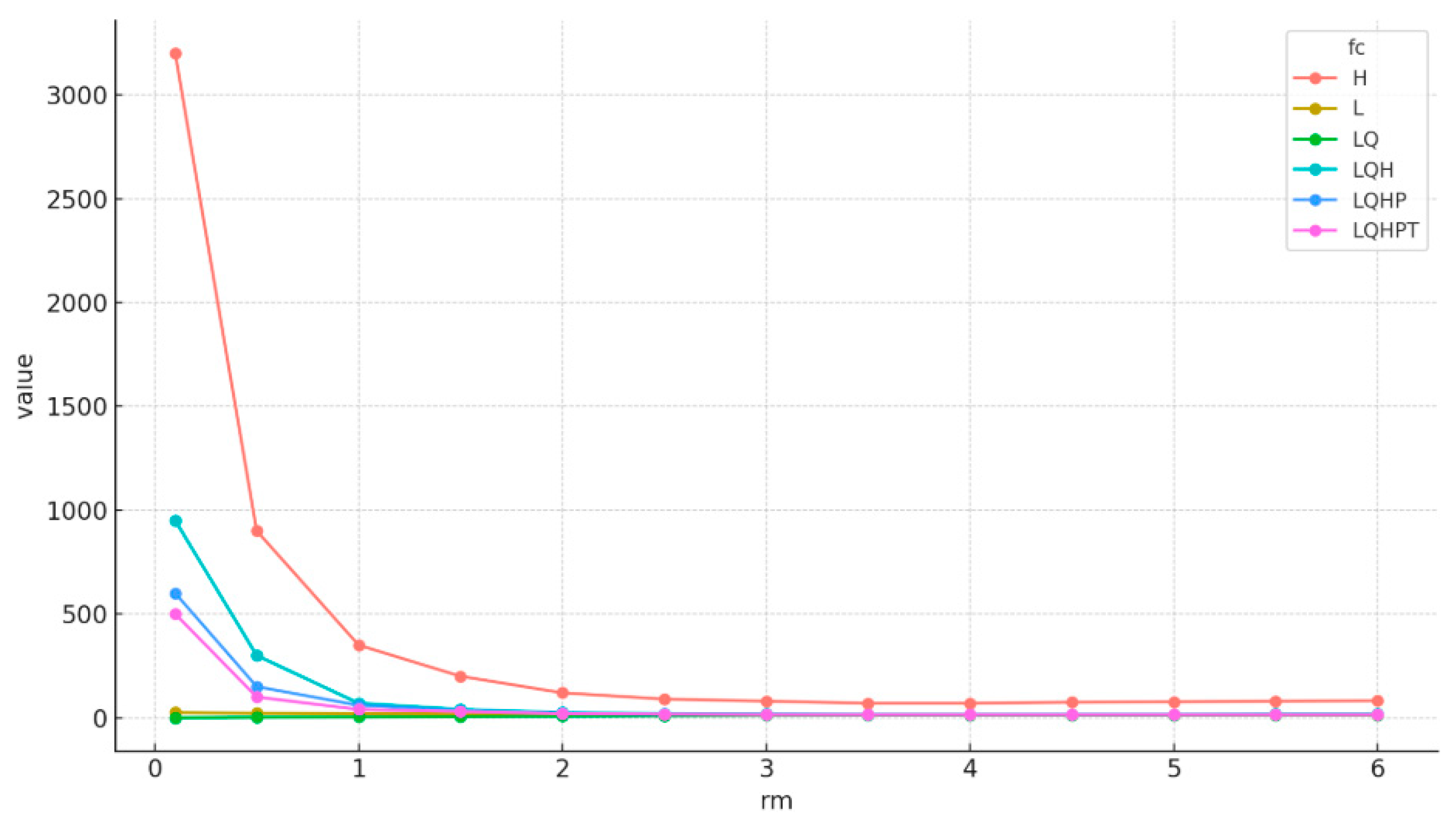
3.1. Optimization and Relative Contributions of the Environmental Variables

The MaxEnt model parameters are optimized using the ENMeval 2.0.5 package. See Figure 8 for Delta.AICc results of the MaxEnt model for C. malabratum under different parameter combinations. This confirms that when RM = 0.1 and FC = LQ, then delta.AICc = 0. This combination of parameters produces the least amount of overfitting and the lowest model complexity, as determined by the Akaike Information Criterion. RM = 0.1 and FC = LQ were thus chosen as the ideal model parameters. The model was built using the optimized parameters to replicate the ideal habitat for C. malabratum.

Within this optimized model, the precipitation of the driest month (bio17), which contributed 28%, was the most significant environmental variable among those considered. However, it is important to interpret this association probabilistically rather than deterministically. As MaxEnt is a correlative algorithm, it does not imply causal physiological responses. Our discussion of environmental drivers, including bio17 and kg1, reflects the statistical association between species presence and environmental predictors, not direct mechanistic limitations. We have accordingly framed our variable interpretation in probabilistic terms, following recommendations from Elith et al. [81] and Merow et al. [83]. Tropical forests exhibit a significant association between water availability during the dry season and species distribution, particularly during droughts [87,88]. Water availability during the dry season has been shown to restrict the ranges of wet-associated species across the neotropics [89] and in WG [90]. This is because new seedlings with shallow root systems cannot access the moister soil levels, and multi-year droughts may impact carbon storage and leaf growth.

The associations between occurrence points and climatic variables such as bio17 (precipitation of the driest quarter) are interpreted in probabilistic terms, acknowledging that MaxEnt is a correlative tool and does not infer physiological mechanisms or causal ecological processes. This approach aligns with the recommendations of Elith et al. [81] and Merow et al. [83], who emphasize that predictor contributions in SDMs should be treated as statistical likelihoods rather than mechanistic determinants of species’ performance. Furthermore, while bio17 emerged as the top predictor in our model, its ecological relevance is interpreted within the broader ecohydrological context of evergreen Lauraceae. Precipitation during dry months has been shown to act as a limiting factor for seedling survival and leaf phenology in related taxa [88], reinforcing its plausibility as a climatic filter for C. malabatrum.

The global CC is typically associated with an increase in overall precipitation levels, resulting from an increase in the air’s moisture capacity. However, local and seasonal patterns may have different trends. Multiple studies have demonstrated a statistically significant decrease in annual precipitation levels in the WG over Kerala [91,92,93]. While statistically significant deviations have not been found for pre-monsoon (dry season) rainfall, an increasing trend in annual drought-like conditions may lead to reduced soil moisture.

The second most important variable is kg1, a simplified layer from the Köppen–Geiger climate classification system, contributing 24.7% to model performance. This system categorizes the Earth into climate groups based on seasonal temperature and precipitation patterns. Originating in 1884 and grounded in the research of climatologist Wladimir Köppen [94], with significant input from climatologist Rudolf Geiger in the 1950s [45,95], this classification employs a system with up to 3 tiers, starting with the five primary groups—A (tropical), B (arid), C (temperate), D (continental), and E (polar)—with subsequent classifications of seasonal precipitation and temperature. The version used in our modeling does not distinguish between tropical savanna subtypes (Aw: dry winter, As: dry summer), grouping them into a single class, whereas kg0 retains this distinction. See Table 3 for classifications of kg2–kg5.

The high contribution of kg1 indicates that C. malabatrum is likely sensitive to broad seasonal climate regimes typical of tropical monsoon (Am) and tropical savanna (Aw/As) climates prevalent across the WG. This supports the species’ ecological affinity for warm and humid monsoonal zones, while suggesting reduced viability in regions with greater seasonality or prolonged dry conditions. Such climatic constraints align with known forest–savanna mosaics in the WG, indicating that C. malabatrum’s distribution may be strongly influenced by tipping points in precipitation and temperature, such as drought or fire, which are key drivers of biome transitions.

Our study area on the western coast of India primarily comprises tropical monsoons (Am) and tropical savannas (Aw), which represent a contiguous biome not present in the study area [45]. A high contribution of the variable kg1 to the suitability of the species implies its endemicity to a relatively narrow range of temperature and precipitation combinations and its unviability beyond this limit in the tropical savanna. This is because while tropical savannas are highly ecologically diverse and provide functions such as food to herbivores, they are tree-limited. In recent studies, it has been suggested that both tropical forests and savannas could represent alternative ‘stable states’ with transitions occurring at ‘tipping points’ that are either climatic (shifts in temperature and precipitation) or human-mediated, such as fires [96,97,98].

The WG already contains examples of such ‘mosaic’ landscapes in the Nilgiris—shola tropical forests interspersed with grasslands [99], albeit within the Am classification. Paleoenvironmental studies within the WG have shown evidence of such alternate stable states [100], as well as vegetation responses to changing monsoon patterns, ranging from intense wet periods with Myristica swamps to cool and dry periods with drought-tolerant species [101]. Similarly, radiocarbon studies of peat samples from within Nilgiris indicated an intense fire episode ~3500 years ago, coinciding with the expansion of grasslands and the migration of pastoralist tribes to the region [102]. Overall, fire, precipitation, and other environmental drivers determine the transitions in vegetation and the establishment of alternate stable states or mosaic landscapes within our study region, including forests and savannas. However, for the continued viability of the species, the study area must be maintained within the tropical monsoon (Am) classification.

The three critical environmental variables in order of contribution are landcover, pet_4, and bio4 (see

Table 5. Environmental variable contribution in the model building of C. malabatrum.

Variable	Percent Contribution	Permutation Importance
bio17	28	14.1
kg1	24.7	3.4
landcover	11.9	1.1
pet_4	6.7	1.7
bio4	5.6	23.6
ai_yr	4.8	1
npp	2.9	30.4
bio12	2.3	7.2
slope_india	2.1	0.5
bio1	2	0.1
pet_7	2	1.6
bio18	1.4	3.4
bio3	1.3	0.4
pet_6	1.3	1
bio2	1	2.3
alt	0.7	3.7
kg0	0.5	1.6
india_aspect	0.4	1.6
in_water	0.3	0.5
ind_ndvi	0.2	0.7

). The land cover prepared from acquired satellite imagery in our analysis is a constant—we have not projected land cover changes across years and scenarios (explained in Section 2.4). Regardless of its influence, land cover changes underscore the importance of monitoring land-use as a critical conservation strategy. Globally, land cover change poses a significant threat to tropical biodiversity [4,103,104]. Pet_4 (monthly potential evapotranspiration in April) and bio4 (temperature seasonality) are related to changes in seasonal air temperatures influenced by CC (the ‘pet_’ variable referring to monthly potential evapotranspiration is appended by a number corresponding to the month of the year, 1 through 12, and ‘pet’ refers to the annual potential evapotranspiration—refer to Table 3). The individual contributions of the following 15 variables, regarding their influence on the ecological model, are less than 5%; therefore, we focus our attention on the five most important variables—bio17, kg1, landcover, pet_4, and bio4.

3.2. Current Distribution and Range of C. malabatrum

The current suitable habitats of C. malabatrum have been disaggregated into three categories—Suitable, Highly suitable, and Very highly suitable—at 0.2 increments of p > 0.4. (See

Table 6. Current habitat suitability of C. malabatrum in the 25 districts, both in terms of percentage and km².

Habitat Type	p-Value	Current Potential Distribution (Km2)	Cinnamomum malabatrum (%)
Unsuitable habitat	0.0–0.2	51,387.59	56.43%
Barely suitable habitat	0.2–0.4	15,510.36	17.03%
Suitable habitat	0.4–0.6	11,249.84	12.35%
Highly suitable habitat	0.6–0.8	8011.03	8.80%
Very highly suitable habitat	0.8–1.0	4912.16	5.39%
		Total—91,070.98	100.00%

). The highly and very highly suitable regions are almost exclusively located in the SWG and the coastal parts and midlands of the southern districts of Kerala (see Figure 5). Current ‘highly suitable’ and ‘very highly suitable’ areas above 11° N are restricted to a specific northwest–southeast-trending series of high-altitude locations (11.3°–11.5° N, 76.20–76.50° E), concentrated within the New Amarambalam Wildlife Sanctuary (11.34° N, 76.40° E). Cinnamomum malabatrum is also prevalent in the high-elevation slopes of SWGs, such as those in the Agasthyamalai Biosphere Reserve (ABR) and Periyar National Park (PNP) (9.46° N, 77.22° E). Among the total study area of 25 districts, ~75% of the area is unsuitable (56.43% unsuitable and 17.03% barely suitable), and <25% is ideal for the species.

The SWG, in particular, is a center of diversity for Cinnamomum—16 out of 18 species have been reported to be endemic to the region. Recent research has described (a) new species—C. agasthyamalayanum [105], C. nilagiricum [106], and C. gamblei [107]; (b) species with expanded ranges—C. Litseaefolium [108] and that of the rediscovered species—C. goaense [109], and C. heyneanum [110]. Another locus of high suitability for the species and a region from which a cluster of occurrence records was obtained (see Figure 1) is the coastal plains of southern Kerala, specifically from the Alappuzha district. These are the ‘sacred groves’, indigenous community-conserved areas containing remnants of primary forests with significant biodiversity. The species has been reported in 16 sacred grove sites across Kerala [111]. An extensive survey of 1128 sacred groves across the Alappuzha district reported considerable floristic diversity, comprising 127 families, 493 genera, and 687 species [112].

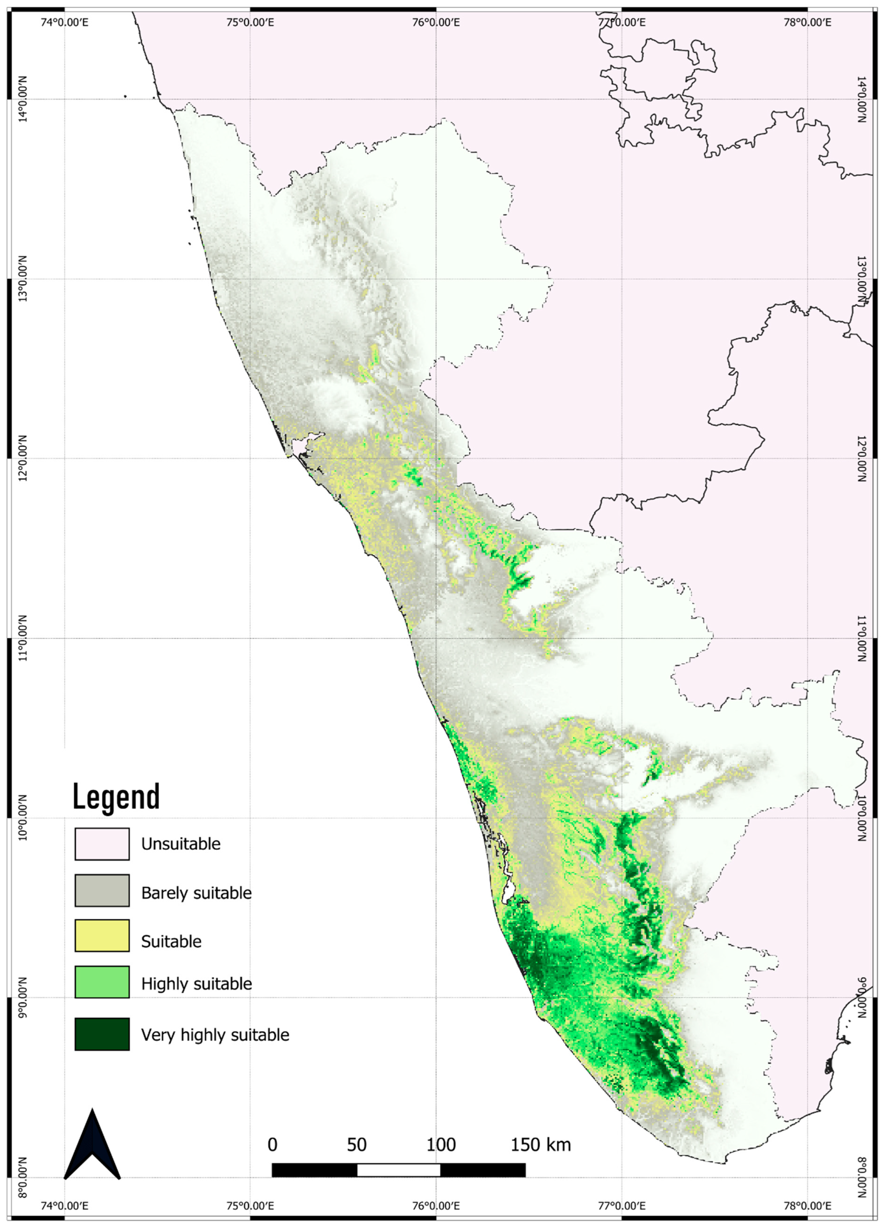
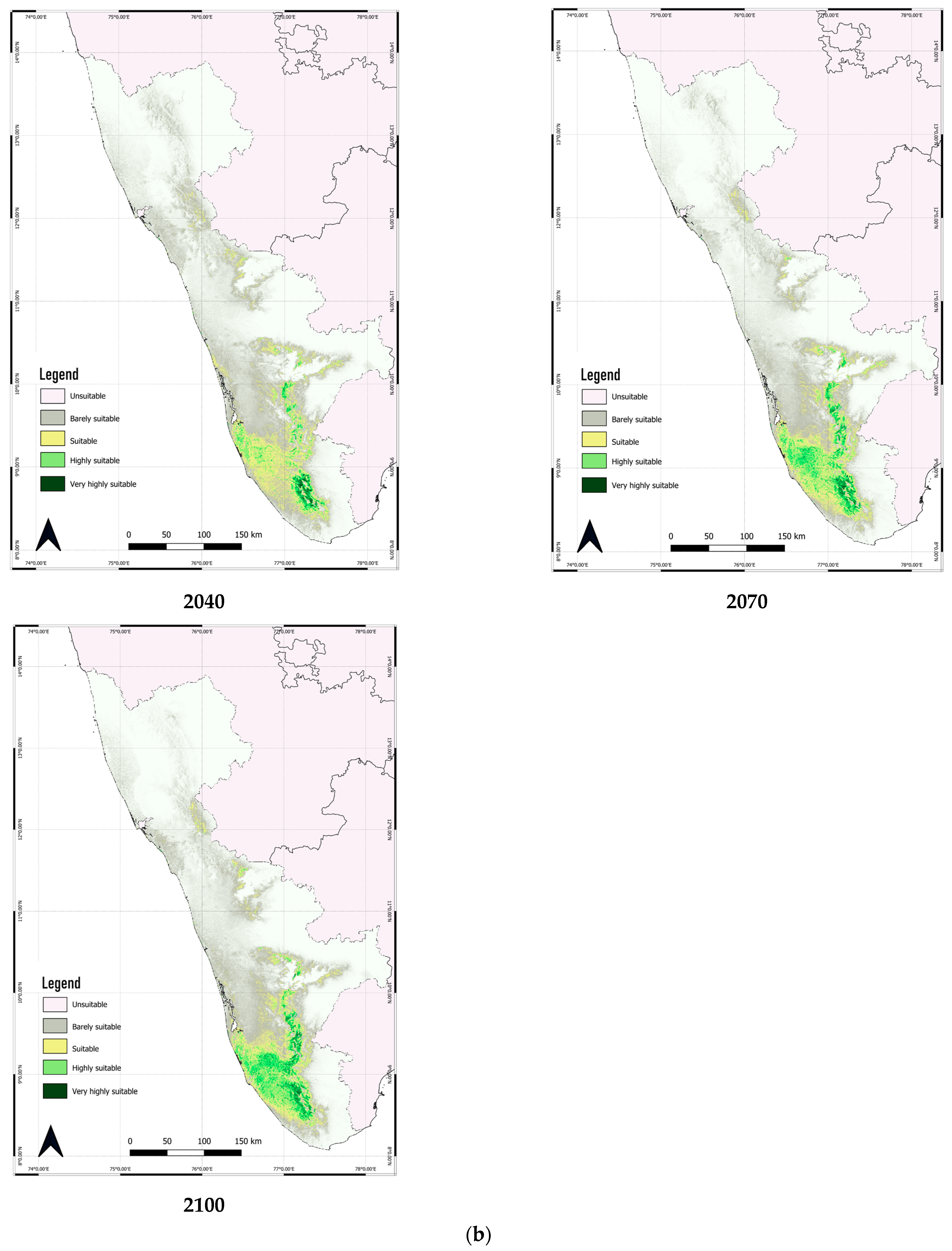
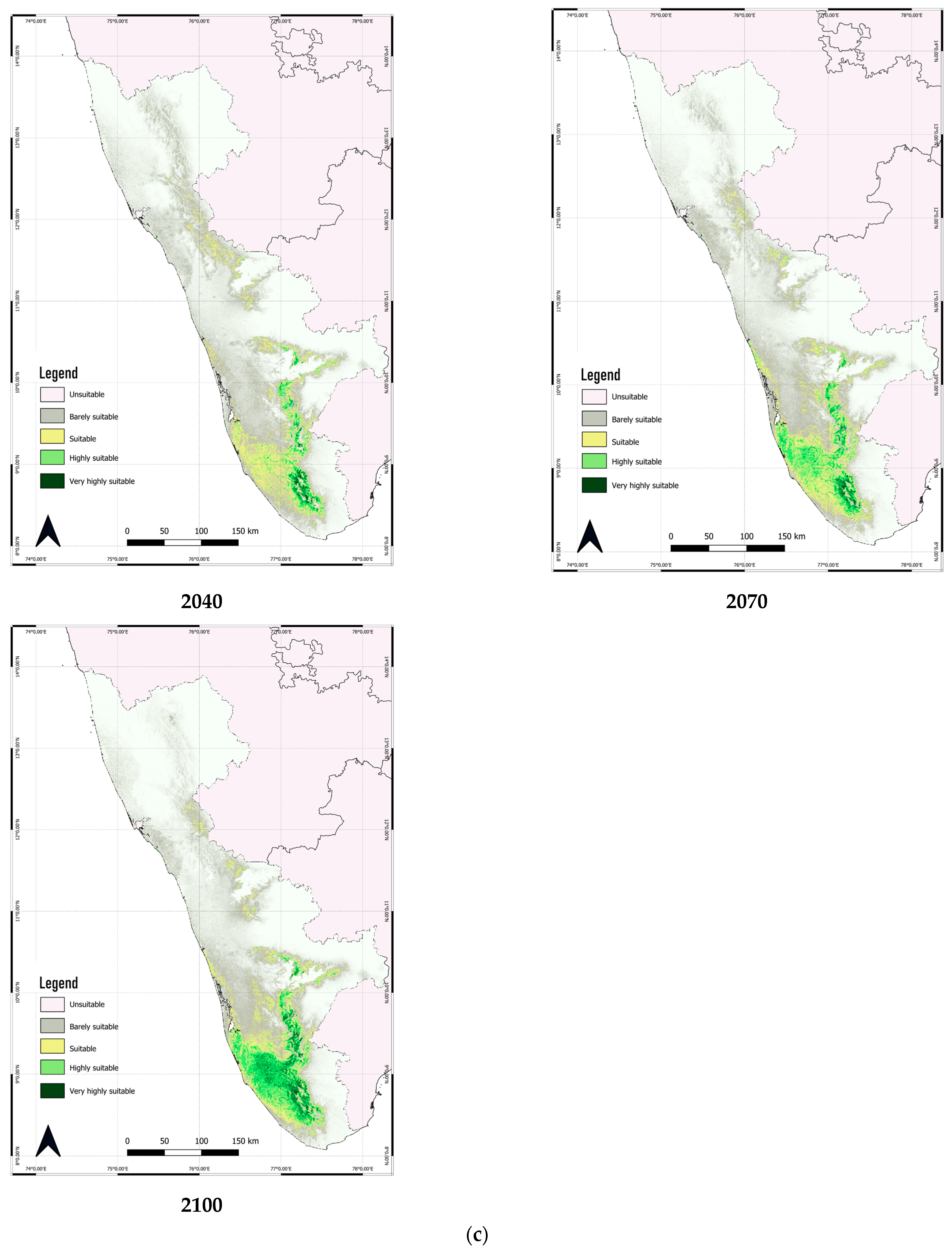
3.3. Predicted Distribution of C. malabatrum

The future habitat projections for C. malabatrum exhibit considerable variation across SSP scenarios, years, and suitability classes, with a consistent pattern of a reduction in suitable classes (greater than 0.4) and an increase in unsuitable classes (less than 0.4) (see

Table 7. Habitat suitability (%) of C. malabatrum under different projected climate scenarios.

Cinnamomum malabatrum		2040			2070			2100
Habitat Class	Current	SSP1_2.6	SSP3_7.0	SSP5_8.5	SSP1_2.6	SSP3_7.0	SSP5_8.5	SSP1_2.6	SSP3_7.0	SSP5_8.5
Unsuitable	51,387.59	59,164.27	61,637.63	59,777.97	65,507.84	64,502.15	60,302.32	64,946.41	62,632.37	61,553.33
Barely suitable	15,510.36	16,169.58	15,872.00	16,996.57	13,525.94	12,704.01	15,046.71	12,618.02	13,670.93	12,064.17
Suitable	11,249.84	8801.76	8564.04	9240.97	7769.93	6641.15	7720.19	7213.55	7052.54	7649.38
Highly Suitable	8011.03	5376.65	4333.86	4030.38	3570.11	6067.07	6588.89	4658.42	6223.03	6302.27
Very highly suitable	4912.16	1558.71	663.44	1025.09	697.16	1156.60	1412.87	1634.58	1492.11	3501.82

). The predicted suitable regions are almost exclusively across southern Kerala, with ‘Suitable’ (0.4–0.6) areas in the midlands and coastal regions and ‘Highly suitable’ and ‘Very highly suitable’ (0.6–0.8 and 0.8–1.0, respectively) holdouts at higher elevation slopes of the SWG, such as the Agasthyamalai Biosphere Reserve (ABR). The distribution areas have shifted almost entirely southward, resulting in a substantial increase in unsuitable areas and a decrease in suitable areas across all scenarios and periods (see

Table 8. Change in habitat suitability (from present day) of Cinnamomum malabatrum under different projected climate scenarios (km²).

Cinnamomum malabatrum	2040			2070			2100
Habitat Class	SSP1_2.6	SSP3_7.0	SSP5_8.5	SSP1_2.6	SSP3_7.0	SSP5_8.5	SSP1_2.6	SSP3_7.0	SSP5_8.5
Unsuitable	15.13%	19.95%	16.33%	27.48%	25.52%	17.35%	26.39%	21.88%	19.78%
Barely suitable	4.25%	2.33%	9.58%	−12.79%	−18.09%	−2.99%	−18.65%	−11.86%	−22.22%
Suitable	−21.76%	−23.87%	−17.86%	−30.93%	−40.97%	−31.38%	−35.88%	−37.31%	−32.00%
Highly suitable	−32.88%	−45.90%	−49.69%	−55.44%	−24.27%	−17.75%	−41.85%	−22.32%	−21.33%
Very highly suitable	−68.27%	−86.49%	−79.13%	−85.81%	−76.45%	−71.24%	−66.72%	−69.62%	−28.71%

).

In eight out of nine scenarios (see Figure 6a–c), there is a noticeable clustering of high-suitability areas in the ABR. In three of the nine scenarios (SSP 1—2.6, 2040, 2100 and SSP 5—8.5, 2100), there are high suitability holdouts in a north–south trending cluster of points (between 8.4° N, 77.5° E and 10° N, 77° E) centered around the PNP. In just one of the nine scenarios (SSP 5—8.5, 2100), there is a diffuse spread of suitable and highly suitable areas in the midlands of Pathanamthitta (9.07°–9.48° N and 76.47°–77.28° E) and Kollam districts (8.76°–9.17° N and 76.45°–77.26° E) of Kerala, east of ABR (see Figure 6c).

The Agasthyamalai Biosphere Reserve has been a protected area since 2001, with additional conserved areas added since then. It has high endemic diversity, which experienced extensive deforestation in the eight decades preceding its protection, particularly between 1920 and 1973 [113]. Invasive tendencies of the local bamboo species Ochlandra travancorica (Poaceae) in the core area have also been reported [113], despite extensive conservation efforts that led to nearly zero deforestation between 2001 and 2012 [113].

PNP (also known as the Periyar Tiger Reserve, PTR) spans an area of 777 sq. km and has been protected as a wildlife sanctuary since 1950. The core area of 350 sq. km has been designated as a national park since 1982. [114]. It has been recognized to hold a collection of multiple endangered and endemic fauna and flora. The collection of non-timber forest products (NTFP), including that of C. malabatrum, has been reported from the region [115]. Recent conservation efforts have had a positive impact, including bringing former poachers and local communities on board for enhanced monitoring [115]. The distribution of C. malabatrum in the future will depend on continued protection efforts, which is also true for ABR.

The projections for 2100 across all three scenarios show suitable regions to the north of PNR (9.46°N, 77.22° E) and east of Idukki Wildlife Sanctuary (9.78° N, 76.96° E), which encompasses Cardamom Hill Reserves (CHR) (9.86° N, 77.15° E) and smaller towns such as Vandiperiyar (9.57° N, 77.05° E), Kumli (9.60° N, 77.16° E), Ayyappankovil (9.69° N, 77.04° E), and Kattappana (9.75° N, 77.11° E). C. malabatrum has been reported as an endemic shade tree in cardamom plantations [116], and the dangers to biodiversity due to intensive cardamom cultivation are prevalent. Ensuring the distribution of the species in this region would thus require consideration of the interests of multiple stakeholders.

Similarly, Vandiperiyar, Kumli, Ayyappankovil, and Kattappana have their economies and primary sources of livelihood centered around highland plantation agriculture; the dangers to biodiversity resulting from land-use change have been noted over the years [117]. The Idukki district in Kerala, where these areas are located, has been the locus of multiple local protests against perceived threats to livelihoods from increased conservation efforts. Therefore, any conservation efforts that rely solely on increasing protected areas would be sociopolitically infeasible.

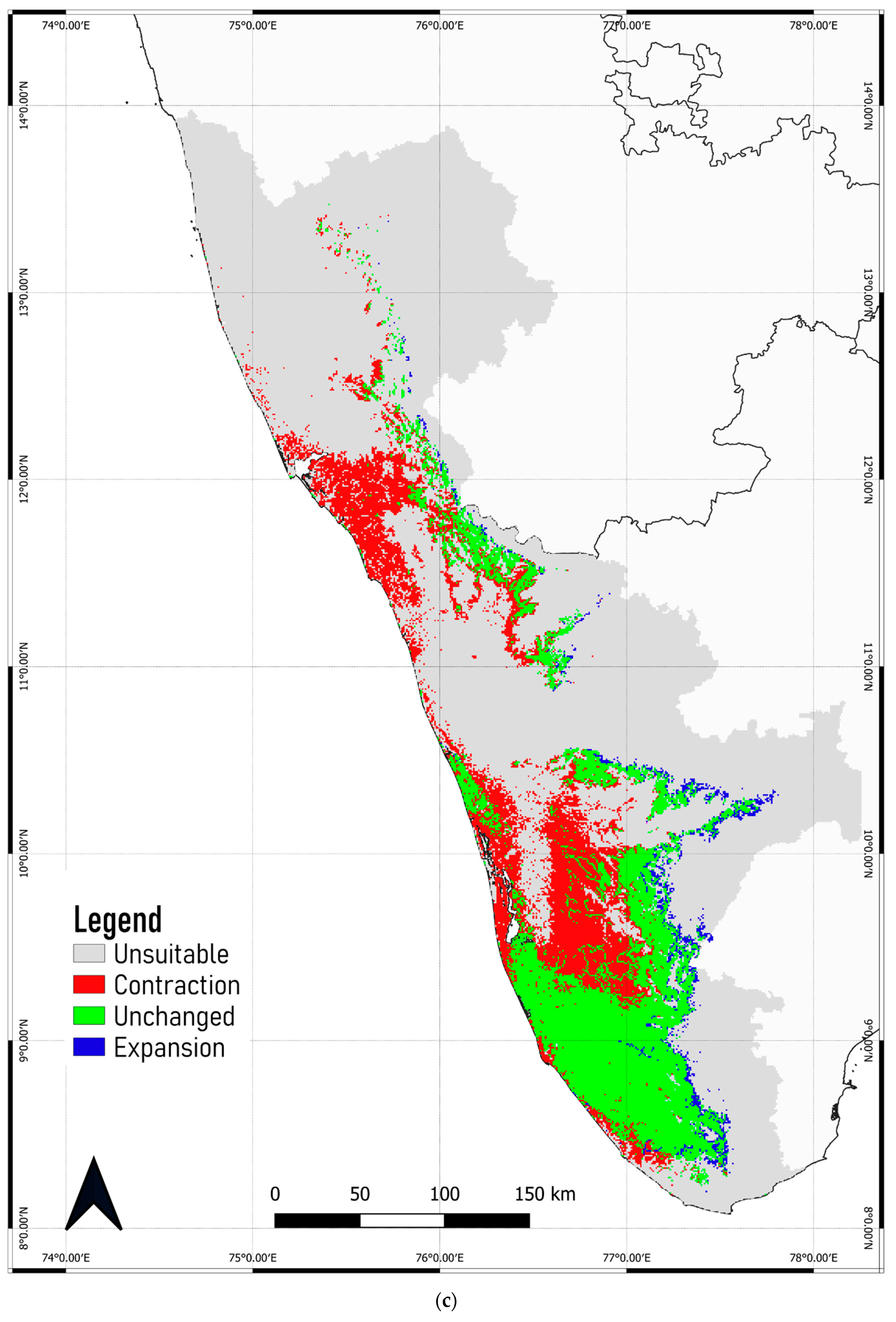
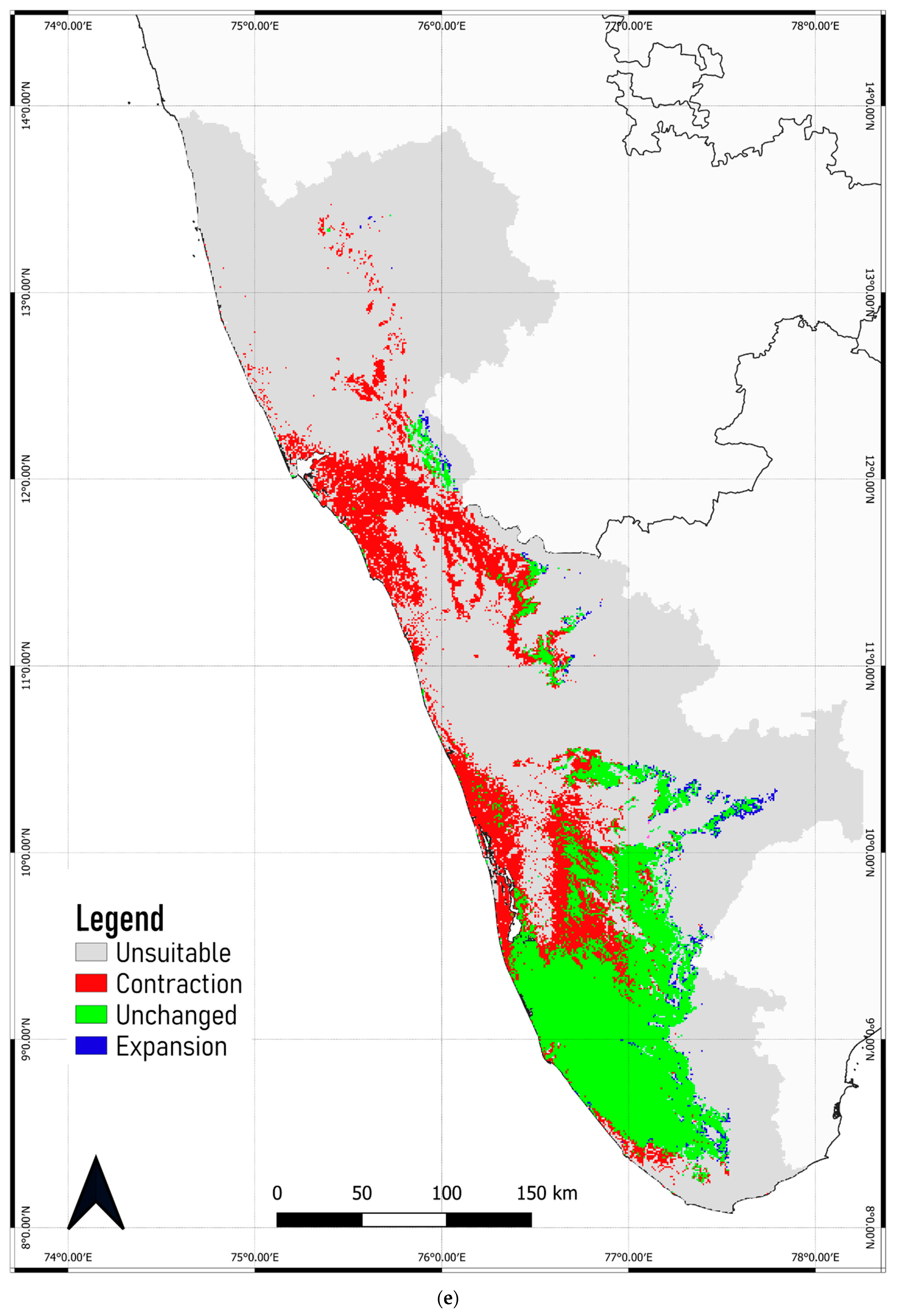
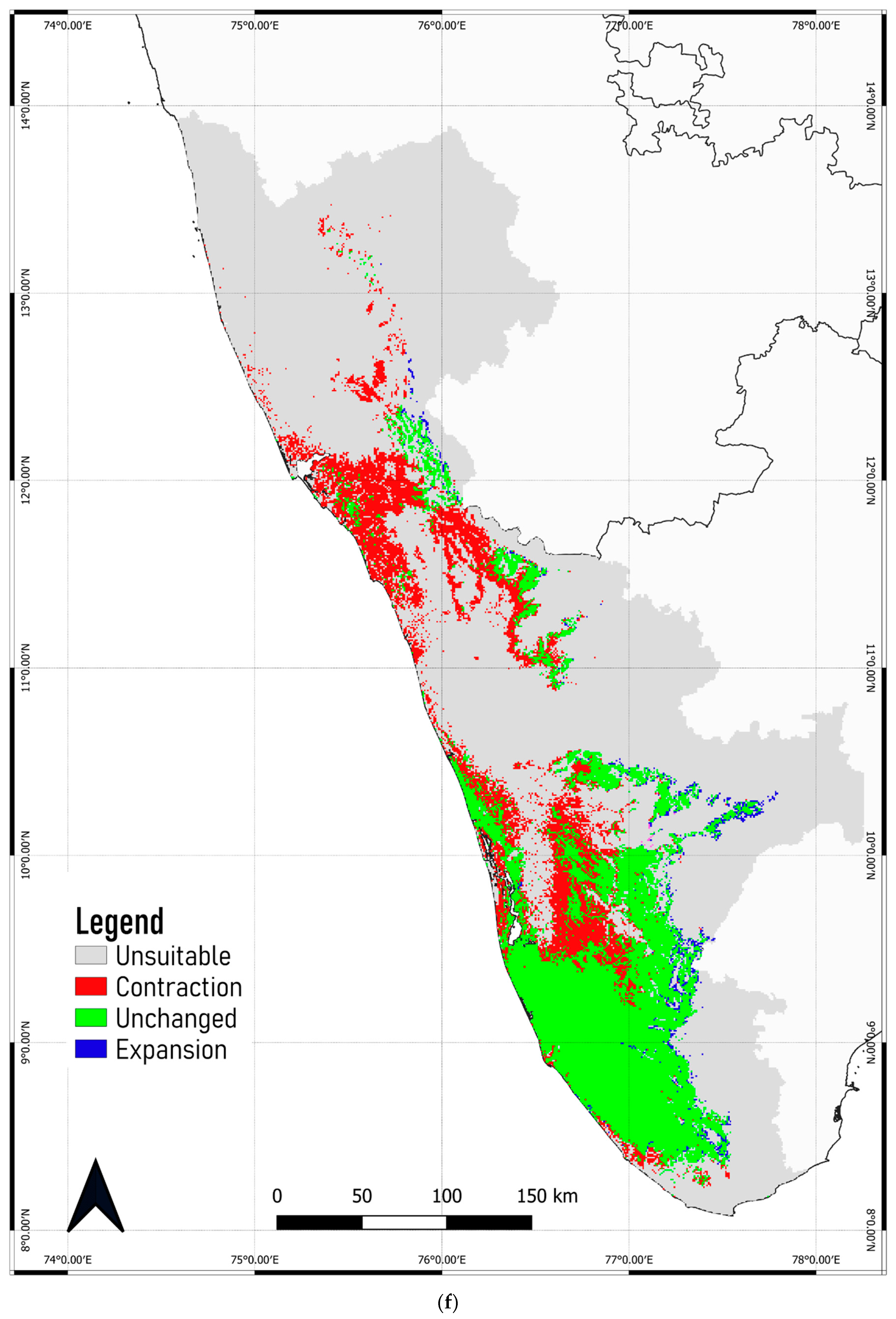
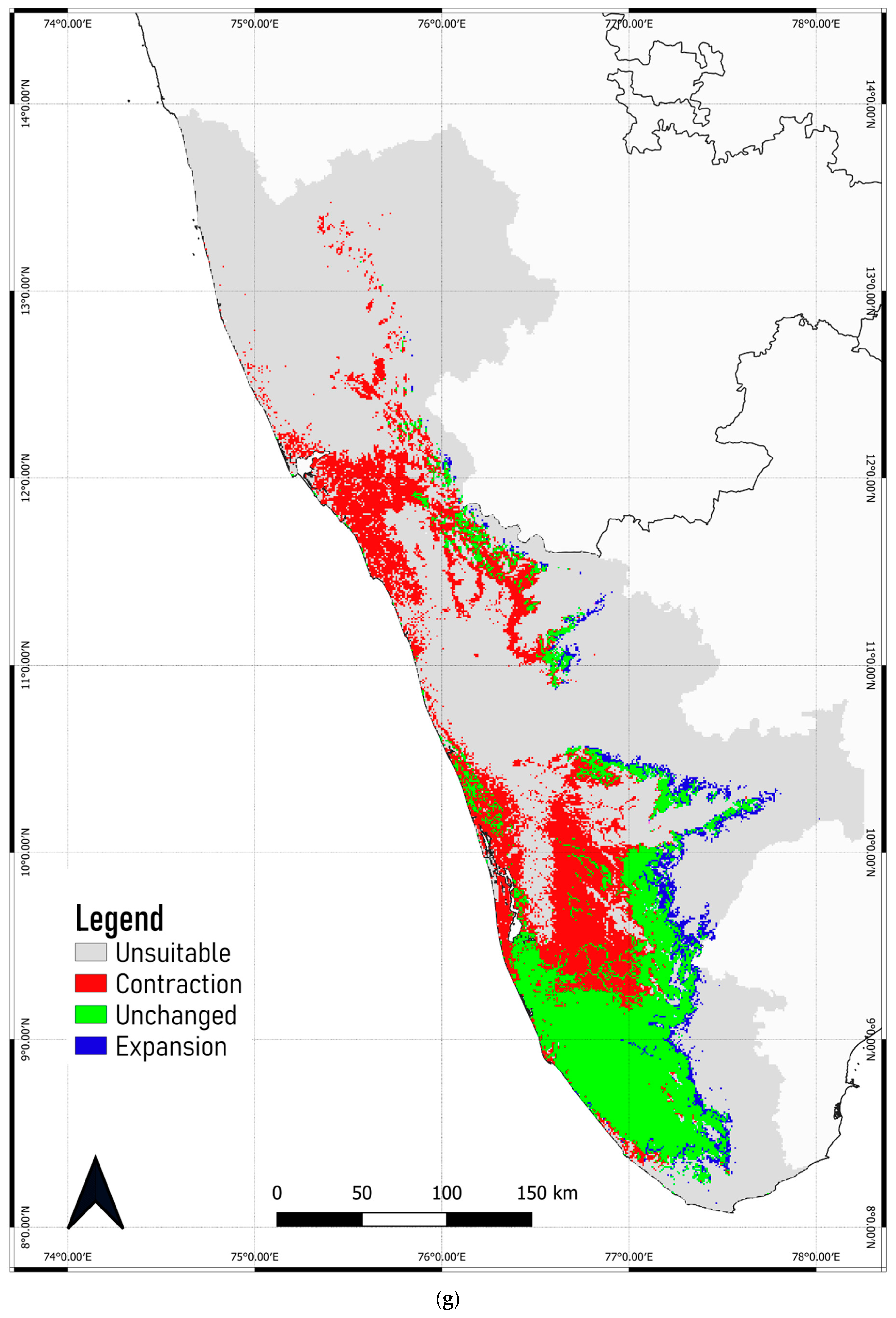
3.4. Predicted Shift in the Range of C. malabatrum

All range shift predictions for C. malabatrum (see Figure 7a–i) show a noticeable contraction of ‘Highly suitable’ and ‘Very Highly suitable’ areas in the northern regions in the present range—northern Kerala and southern Karnataka (above 11° N). In all scenarios, there is a substantial contraction in the midlands and coastal regions, particularly in the Alappuzha district in Kerala. However, this is most pronounced in three scenarios—SSP 5—8.5 in 2040, SSP 1—2.6 in 2070, and SSP 1—2.6 in 2100. Where they exist, possibilities of expansion are restricted to the higher elevations of the SWG.

Significant range contraction occurred in areas above 11° N across all scenarios (11–13° N and 75–77 ° E). In particular, this has occurred in lowlands and the coastal regions, which currently harbor areas of medium suitability (0.4–0.6). The prognosis is decidedly more mixed for the elevated slopes of the WG, above 400 m (11.3–12.5–12.5–N, 75.50–76.50–E). Only two scenarios (2040—SSP1—2.6 and SSP5—8.5) have unchanged ranges across the elevated region, with range contraction occurring only closer to the valleys. Two other scenarios (SSP1—2.6 in 2070 and 2100) depict more pessimistic versions of the previous two, with range contraction extending into higher elevations and a small selection of areas maintaining unchanged ranges. All other scenarios (2040— SSP3—7.0; 2070—SSP3—7.0, and SSP5—8.5; 2100—SSP3—7.0 and SSP5—8.5) show a complete range contraction in the middle of this high-elevation area (11.3°–12.0° N, 76°–76.50° E) and two ‘Unchanged’ holdouts on either side (centered at 12° N, 76° E and 11.3° N, 76.50° E). Across all scenarios, only minuscule possibilities of range expansion exist, situated along the eastern (i.e., higher elevation) edges of the ‘Unchanged’ regions. Only one scenario (2100—SSP1—2.6, (see Figure 7g)) shows the most significant possibility of expansion into parts of Tamil Nadu, including the Cumbum valley (9.75° N, 77.30° E).

The regions in the study area comprising the midlands and coastal areas of the southern districts of Kerala (south of 11° N) paint a mixed picture across range shift scenarios. In all the cases, the regions of the Thiruvananthapuram, Pathanamthitta, Kottayam, and Alappuzha districts (Table 1) between 8.3° and 9.3° N and between 76.3° and 77.3° E retain the most significant proportion of ‘Unchanged’ status. Given that this region currently has extensive coverage of areas with suitability above 0.6 (Figure 4), the situation appears promising. However, this must be considered alongside the future distribution maps (see Figure 6a–c), where across the region, we observe a shift from the two categories above to ‘Suitable’, a dynamic not captured by our range shift maps. Across all the scenarios, we also observe range contraction in coastal areas (containing the ‘sacred groves’), with the most pronounced decline in five out of the nine scenarios (2040—SSP3—7.0, SSP5—8.5; 2070—SSP1—2.6, SSP3—7.0; and 2100—SSP1—2.6, SSP3—7.0).

The midlands across the Kottayam, Ernakulam, Idukki, and Pathanamthitta districts of Kerala (9.0–10.5° N, 76.50–77° E) show varying responses. The most marked contraction occurs in 7 out of 9 scenarios, except for SSP3—7.0 and SSP5—8.5 in 2100. However, this contraction is partially offset by an ‘unchanged’ status in a small region centered at 9.9° N, 76.7° E in four of these seven scenarios. Specifically, the ‘unchanged’ status is observed in 2040 under SSP1—2.6 and SSP3—7.0, and in 2070 under SSP3—7.0 and SSP5—8.5. In all scenarios, range expansions are restricted to the eastern high-elevation edges. Two scenarios (2100—SSP1—2.6 and SSP5—8.5) show the most significant possibility of expansion across the entire eastern edge (8.0–10.5° N), as shown in

Table 9. Range shift analysis of C. malabatrum under different climate scenarios in Km².

	2040			2070			2100
Range Shift Category	SSP1_2.6	SSP3_7.0	SSP5_8.5	SSP1_2.6	SSP3_7.0	SSP5_8.5	SSP1_2.6	SSP3_7.0	SSP5_8.5
Range expansion	1100.12	567.34	1266.19	506.64	668.50	730.88	1931.31	459.44	1884.11
Unsuitable	65,849.26	66,382.04	65,678.13	66,437.67	66,275.82	66,213.44	65,018.90	66,489.94	65,060.21
Unchanged	14,578.00	12,938.36	13,009.18	11,511.17	13,171.88	14,953.98	11,538.14	14,221.41	15,512.89
Range contraction	9543.60	11,183.24	11,117.48	12,615.50	10,954.79	9172.68	12,582.62	9900.19	8613.77

.

While these midland and coastal districts show ‘unchanged’ status to a high degree in our projections, it is critical to note that this may over-represent actual persistence potential, particularly in heavily fragmented landscapes of districts such as Kottayam and Alappuzha. Given the intensity of land-use change in these districts, characterized by urbanization, plantation agriculture, and habitat discontinuity, our fundamental niche model (as elaborated in Section 2.4) likely includes areas where real-world survival and regeneration of C. malabatrum may be ecologically implausible. The apparent persistence of suitability in these zones should therefore be interpreted cautiously. As our model estimates the species’ fundamental niche, it includes areas that may no longer be ecologically viable due to human transformation. Future efforts that integrate land-use projections aligned with SSPs could provide more comprehensive forecasts of realized habitat availability.

When we examine the range shift maps in conjunction with a district map of our study area, it becomes clear that the range contraction is restricted to specific regions across all scenarios. By identifying these districts, more targeted conservation efforts could be suggested. Kerala already has the institutional capacity to direct biodiversity conservation at the decentralized level through biodiversity management committees [118].

We extracted a separate vector map of the four districts in Kerala where the range contraction seemed to be concentrated—Kannur, Kozhikode, Kottayam, and Idukki. By intersecting this map with the range shift maps, we could isolate the range contraction area within these districts and compare it with the overall range contraction area (see

Table 10. Districts where the range contraction of C. malabatrum is concentrated.

	2040			2070			2100
Range Contraction in Kozhikode, Kannur, Kottayam, and Idukki Districts	SSP1_2.6	SSP3_7.0	SSP5_8.5	SSP1_2.6	SSP3_7.0	SSP5_8.5	SSP1_2.6	SSP3_7.0	SSP5_8.5
Range contraction (sq.km)	4779.78	5142.22	5410.36	5698.18	4701.88	4432.92	5658	4189.38	3747.4
% total range contraction	51.21%	47.03%	49.68%	46.13%	43.74%	49.36%	45.98%	43.23%	44.31%

). As shown in the table, 43–51% of all range contractions across all the scenarios are in these four districts.

Although our findings offer strong proof of C. malabatrum’s range contraction and southward shifts due to CC, a thorough analysis reveals more significant ecological and conservation ramifications. The species’ high sensitivity to monsoonal regimes (kg1) and dry-season precipitation (bio17) highlights how ecohydrological thresholds limit its niche, which is consistent with theories of environmental envelopes and climatic filtering [88,89]. According to Hirota et al. [96], these niche constraints imply that C. malabatrum might experience nonlinear reactions to gradual CC, particularly in areas that are getting close to ecological tipping points.

Further, our results are consistent with frameworks for climate-smart conservation planning, which prioritize dynamic prioritization in response to anticipated changes in species distributions [119]. There is an urgent need to mainstream community-conserved areas into regional biodiversity policies, given the expected decline in sacred groves and midland habitats in the future. We recognize that static land-use layers and the lack of dynamic biotic interactions may overestimate the persistence potential in fragmented habitats, despite our modeling employing a fundamental niche approach [120].

Given these considerations, conservation strategies need to be integrative and multi-scale, incorporating indigenous stewardship, conflict-sensitive planning in agricultural frontiers, and assisted regeneration in sacred groves. According to Gadgil et al. [121], these are particularly important in WG landscapes where the social-ecological context is complicated and disputed. Our results ultimately highlight the need for climate vulnerability assessments to critically examine the practical viability of conservation implementation under sociopolitical constraints in addition to quantifying exposure and risk.

4. Adaptation Strategies for the Conservation of C. malabatrum

The following are the adaptation strategies suggested for the conservation of C. malabatrum.

(a)

The relatively widespread distribution of C. malabatrum (as opposed to other species with limited suitability and endemicity within WG) in the Malabar midlands and coastal plains is unique. These are also the regions where the maximum range contraction is projected to occur across scenarios and time periods. Therefore, any conservation strategy for C. malabatrum should focus on Malabar midlands and coastal plains because conservation efforts here may prove more accessible in some respects.

(b)

Informal protected areas and traditions (such as sacred groves) may be as valuable as protected reserves in conserving biodiversity, as suggested by [122].

(c)

Cinnamomum malabatrum is most widely reported within the Malabar plains in the ‘sacred groves’ of Kerala, a type of Indigenous Community Conserved Area, as mentioned in Section 3.2. These areas face challenges in Kerala, primarily due to anthropogenic pressure for urbanization and land-use conversion. The improved management and protection of these resources could aid in conserving not only C. malabatrum but also threatened and endangered species, such as Myristica.

(d)

Globally, fragmentation due to land-use conversion significantly impacts tropical tree species. Although the Malabar plains are densely populated, C. malabatrum is at risk of habitat loss due to deforestation, land degradation, and commercial exploitation. This study confirms that precipitation during the driest month is a key ecological variable that stresses C. malabatrum.

(e)

In a study from Nicaragua related to tropical dry forest restoration, irrigation and fertilization were positively correlated with seedling quality and were suggested to improve posttransplant results [123]. A similar study in a seasonally moist forest in Peru revealed that irrigation improved the survival and growth of young seedlings and the growth of older seedlings. These strategies may also benefit our study area, for example, through the social forestry department in Kerala.

(f)

The relationships of indigenous and tribal communities with their surrounding ecosystems and the importance of traditional knowledge, beliefs, and practices for biodiversity conservation have been well documented over the past few decades [121]. The economic importance of C. malabatrum to the Kattunaikka tribe has been mentioned previously [25]. We suggest new policy initiatives to initiate and improve local markets and institutions in SWG. Furthermore, indigenous tribal groups must be included as key stakeholders, which could help conserve the species.

We thus recommend a four-pronged conservation strategy for C. malabatrum—(1) protection of sacred groves in the Malabar plains; (2) policies to prevent indiscriminate land-use change; (3) afforestation/reforestation with supplemental irrigation during summer months; and (4) community conservation strategies within protected areas.

5. Conclusions

In conclusion, the impact of CC on the distribution of C. malabatrum within the WG has implications for biodiversity, cultural practices, and local economies. The findings, rooted in extensive field data and advanced modeling techniques, underscore the urgency of proactive conservation measures.

The predicted range shifts and contraction of suitable habitats for C. malabatrum indicate significant challenges ahead, especially in the Malabar midlands and coastal plains, areas of high endemicity for the species. This calls for targeted conservation interventions in these regions.

The proposed adaptation strategies, including protecting sacred groves, implementing sustainable land-use policies, promoting afforestation efforts with irrigation support, and fostering community engagement, provide a comprehensive framework for conservation. Emphasizing the importance of traditional knowledge and ecosystem stewardship by indigenous communities is essential for the successful implementation of these strategies.

As the global community faces the challenges of CC, biodiversity conservation, and sustainable development, it is essential to recognize the interconnectedness of ecological, cultural, and economic factors. The proposed conservation strategies offer a holistic approach that addresses the protection of a culturally and ecologically significant species, contributing to broader ecosystem resilience and community well-being in the face of environmental change.

In conclusion, this study serves as a clarion call for concerted action and collaboration among researchers, policymakers, local communities, and conservation practitioners to safeguard the delicate balance of nature and the ecosystem. Implementing these strategies plays an essential role in preserving the ecological and cultural heritage of the Malabar region.

References

1. IPCC. Climate Change 2022–Impacts, Adaptation and Vulnerability; Cambridge University Press (CUP): Cambridge, UK, 2023. [Google Scholar]
2. Sintayehu, D.W. Impact of climate change on biodiversity and associated key ecosystem services in Africa: A systematic review. Ecosyst. Health Sustain. 2018, 4, 225–239. [Google Scholar] [CrossRef]
3. Habibullah, M.S.; Din, B.H.; Tan, S.-H.; Zahid, H. Impact of climate change on biodiversity loss: Global evidence. Environ. Sci. Pollut. Res. 2021, 29, 1073–1086. [Google Scholar] [CrossRef] [PubMed]
4. Nunez, S.; Arets, E.; Alkemade, R.; Verwer, C.; Leemans, R. Assessing the impacts of climate change on biodiversity: Is below 2 °C enough? Clim. Change 2019, 154, 351–365. [Google Scholar] [CrossRef]
5. Segan, D.B.; Murray, K.A.; Watson, J.E. A global assessment of current and future biodiversity vulnerability to habitat loss–climate change interactions. Glob. Ecol. Conserv. 2016, 5, 12–21. [Google Scholar] [CrossRef]
6. Obura, D. The Kunming-Montreal Global Biodiversity Framework: Business as usual or a turning point? One Earth 2023, 6, 77–80. [Google Scholar] [CrossRef]
7. Reddy, C.S.; Jha, C.S.; Dadhwal, V.K. Earth Observations based Conservation Prioritization in Western Ghats, India. J. Geol. Soc. India 2018, 92, 562–567. [Google Scholar] [CrossRef]
8. Anitha, K.; Joseph, S.; Chandran, R.J.; Ramasamy, E.; Prasad, S.N. Tree species diversity and community composition in a human-dominated tropical forest of Western Ghats biodiversity hotspot, India. Ecol. Complex. 2010, 7, 217–224. [Google Scholar] [CrossRef]
9. Varikoden, H.; Revadekar, J.V.; Kuttippurath, J.; Babu, C.A. Contrasting trends in southwest monsoon rainfall over the Western Ghats region of India. Clim. Dyn. 2018, 52, 4557–4566. [Google Scholar] [CrossRef]
10. Pramanik, M.; Paudel, U.; Mondal, B.; Chakraborti, S.; Deb, P. Predicting climate change impacts on the distribution of the threatened Garcinia indica in the Western Ghats, India. Clim. Risk Manag. 2018, 19, 94–105. [Google Scholar] [CrossRef]
11. Sen, S.; Gode, A.; Ramanujam, S.; Ravikanth, G.; Aravind, N.A. Modeling the impact of climate change on wild Piper nigrum (Black Pepper) in Western Ghats, India using ecological niche models. J. Plant Res. 2016, 129, 1033–1040. [Google Scholar] [CrossRef]
12. Sony, R.; Sen, S.; Kumar, S.; Sen, M.; Jayahari, K. Niche models inform the effects of climate change on the endangered Nilgiri Tahr (Nilgiritragus hylocrius) populations in the southern Western Ghats, India. Ecol. Eng. 2018, 120, 355–363. [Google Scholar] [CrossRef]
13. Sreekumar, E.; Nameer, P. A MaxEnt modelling approach to understand the climate change effects on the distributional range of White-bellied Sholakili Sholicola albiventris (Blanford, 1868) in the Western Ghats, India. Ecol. Inform. 2022, 70, 101702. [Google Scholar] [CrossRef]
14. Sreekumar, E.R.; Nameer, P.O. Impact of Climate Change on Two High-Altitude Restricted and Endemic Flycatchers of The Western Ghats, India. Curr. Sci. 2021, 121, 1335–1342. [Google Scholar] [CrossRef]
15. Raman, S.; Shameer, T.T.; Sanil, R.; Usha, P.; Kumar, S. Protrusive influence of climate change on the ecological niche of endemic brown mongoose (Herpestes fuscus fuscus): A MaxEnt approach from Western Ghats, India. Model. Earth Syst. Environ. 2020, 6, 1795–1806. [Google Scholar] [CrossRef]
16. Das, M.L.; Bondada, S.; Rajesh, K.; Subrahmanyam, S. Climate change impacts on habitat suitability of Cinnamomum travancoricum (Lauraceae), a critically endangered endemic vascular plant in the Western Ghats, India. Isr. J. Ecol. Evol. 2023, 1, 1–19. [Google Scholar] [CrossRef]
17. Subrahmanyam, S.; Das, M.L.; Kumara, H.N. Climate Change Projections of Current and Future Distributions of the Endemic Loris lydekkerianus (Lorinae) in Peninsular India. In Exploring Synergies and Trade-offs between Climate Change and the Sustainable Development Goals; Springer: Berlin, Germany, 2021. [Google Scholar]
18. Anoop, N.; Babu, S.; Nagarajan, R.; Sen, S. Identifying suitable reintroduction sites for the White-rumped Vulture (Gyps bengalensis) in India’s Western Ghats using niche models and habitat requirements. Ecol. Eng. 2020, 158, 106034. [Google Scholar] [CrossRef]
19. Priti, H.; Aravind, N.; Shaanker, R.U.; Ravikanth, G. Modeling impacts of future climate on the distribution of Myristicaceae species in the Western Ghats, India. Ecol. Eng. 2016, 89, 14–23. [Google Scholar] [CrossRef]
20. Kostermans, A. A Note on Two Species of Cinnamomum (Lauraceae) Described in Hortus Indicus Malabaricus. In Botany and history of Hortus Malabaricus; Oxford IBH: New Delhi, India, 1980; pp. 163–167. [Google Scholar]
21. van Rheede, H.; Casearium, J.; Syen, A. Hortus Indicus Malabaricus Vol 1; Ametelodami: Amsterdam, The Netherlands, 1685. [Google Scholar]
22. Hooker, J.D. Flora of British India, Vol. V; Reeve & Co.: London, UK, 1886. [Google Scholar]
23. Gamble, J.S. Flora of the Presidency of Madras, Vol. II; Botanical Survey of India: Calcutta, India, 1925.
24. Berkes, F. Community conserved areas: Policy issues in historic and contemporary context. Conserv. Lett. 2009, 2, 20–25. [Google Scholar] [CrossRef]
25. Narayanan, M.R.; Mithunlal, S.; Sujanapal, P.; Kumar, N.A.; Sivadasan, M.; Alfarhan, A.H.; Alatar, A. Ethnobotanically Important Trees and Their Uses by Kattunaikka Tribe in Wayanad Wildlife Sanctuary, Kerala, India. J. Med. Plants Res. 2011, 5, 604–612. [Google Scholar]
26. Duguta, T.; Cheriyan, B.V. An Introduction and Various Phytochemical Studies of Cinnamomum Malabatrum: A Brief Review. Pharmacogn. J. 2021, 13, 792–797. [Google Scholar] [CrossRef]
27. Kuttithodi, A.M.; Narayanankutty, A.; Visakh, N.U.; Job, J.T.; Pathrose, B.; Olatunji, O.J.; Alfarhan, A.; Ramesh, V. Chemical Composition of the Cinnamomum malabatrum Leaf Essential Oil and Analysis of Its Antioxidant, Enzyme Inhibitory and Antibacterial Activities. Antibiotics 2023, 12, 940. [Google Scholar] [CrossRef] [PubMed]
28. Soumya, V.; Deepa, S.; Thachil, K.; Saravanan, J.; Hariprasad, R. GC-MS analysis and in silico docking of constituents of Cinnamomum malabatrum against CYP450 17α and CYP450 19 (Aromatase)- Key targets for hyperandrogenism. Drug Res. 2023, 73, 441–447. [Google Scholar] [CrossRef]
29. Ananthakrishnan, R.; SanthoshKumar, E.S.; Rameshkumar, K.B. Comparative Chemical Profiles of Essential Oil Constituents of Eight Wild Cinnamomum Species from the Western Ghats of India. Nat. Prod. Commun. 2018, 13, 1934578. [Google Scholar] [CrossRef]
30. Shylaja, M.; Ravindran, P.; Babu, K.N. Other Useful Species of Cinnamomum. In Cinnamon and Cassia; CRC Press: Boca Raton, FL, USA, 2003; pp. 346–371. [Google Scholar]
31. Qi, S.; Luo, W.; Chen, K.-L.; Li, X.; Luo, H.-L.; Yang, Z.-Q.; Yin, D.-M. The Prediction of the Potentially Suitable Distribution Area of Cinnamomum mairei H. Lév in China Based on the MaxEnt Model. Sustainability 2022, 14, 7682. [Google Scholar] [CrossRef]
32. Zhang, L.; Jing, Z.; Li, Z.; Liu, Y.; Fang, S. Predictive Modeling of Suitable Habitats for Cinnamomum Camphora (L.) Presl Using Maxent Model under Climate Change in China. Int. J. Environ. Res. Public Health 2019, 16, 3185. [Google Scholar] [CrossRef]
33. Costion, C.M.; Simpson, L.; Pert, P.L.; Carlsen, M.M.; Kress, W.J.; Crayn, D. Will tropical mountaintop plant species survive climate change? Identifying key knowledge gaps using species distribution modelling in Australia. Biol. Conserv. 2015, 191, 322–330. [Google Scholar] [CrossRef]
34. Freeman, B.G.; Lee-Yaw, J.A.; Sunday, J.M.; Hargreaves, A.L. Expanding, shifting and shrinking: The impact of global warming on species’ elevational distributions. Glob. Ecol. Biogeogr. 2018, 27, 1268–1276. [Google Scholar] [CrossRef]
35. Pauli, H.; Gottfried, M.; Reiter, K.; Klettner, C.; Grabherr, G. Signals of range expansions and contractions of vascular plants in the high Alps: Observations (1994–2004) at the GLORIA* master site Schrankogel, Tyrol, Austria. Glob. Change Biol. 2006, 13, 147–156. [Google Scholar] [CrossRef]
36. Bucklin, D.N.; Basille, M.; Benscoter, A.M.; Brandt, L.A.; Mazzotti, F.J.; Romañach, S.S.; Speroterra, C.; Watling, J.I.; Thuiller, W. Comparing species distribution models constructed with different subsets of environmental predictors. Divers. Distrib. 2014, 21, 23–35. [Google Scholar] [CrossRef]
37. Luoto, M.; Virkkala, R.; Heikkinen, R.K. The role of land cover in bioclimatic models depends on spatial resolution. Glob. Ecol. Biogeogr. 2006, 16, 34–42. [Google Scholar] [CrossRef]
38. Myers, N.; Mittermeier, R.A.; Mittermeier, C.G.; da Fonseca, G.A.B.; Kent, J. Biodiversity hotspots for conservation priorities. Nature 2000, 403, 853–858. [Google Scholar] [CrossRef]
39. Singh, A.K. Probable Agricultural Biodiversity Heritage Sites in India: XXI. The Malabar Region. Asian Agri-Hist. 2014, 18, 311–341. [Google Scholar]
40. Pascal, J.P.; Ramesh, B.R. Atlas of Endemics of the Western Ghats (India): Distribution of Tree Species in the Evergreen and Semi-Evergreen Forests; Institut Français de Pondichéry: Pondichéry, India, 1997. [Google Scholar]
41. Young, W.; Weckman, G.; Holland, W. A survey of methodologies for the treatment of missing values within datasets: Limitations and benefits. Theor. Issues Ergon. Sci. 2011, 12, 15–43. [Google Scholar] [CrossRef]
42. Lavoie, C. Biological collections in an ever changing world: Herbaria as tools for biogeographical and environmental studies. Perspect. Plant Ecol. Evol. Syst. 2013, 15, 68–76. [Google Scholar] [CrossRef]
43. Kramer-Schadt, S.; Niedballa, J.; Pilgrim, J.D.; Schröder, B.; Lindenborn, J.; Reinfelder, V.; Stillfried, M.; Heckmann, I.; Scharf, A.K.; Augeri, D.M.; et al. The importance of correcting for sampling bias in MaxEnt species distribution models. Divers. Distrib. 2013, 19, 1366–1379. [Google Scholar] [CrossRef]
44. Soberón, J. Grinnellian and Eltonian niches and geographic distributions of species. Ecol. Lett. 2007, 10, 1115–1123. [Google Scholar] [CrossRef]
45. Peel, M.C.; Finlayson, B.L.; McMahon, T.A. Updated world map of the Köppen-Geiger climate classification. Hydrol. Earth Syst. Sci. 2007, 11, 1633–1644. [Google Scholar] [CrossRef]
46. Guisan, A.; Thuiller, W. Predicting species distribution: Offering more than simple habitat models. Ecol. Lett. 2005, 8, 993–1009. [Google Scholar] [CrossRef]
47. Hirzel, A.H.; Le Lay, G. Habitat suitability modelling and niche theory. J. Appl. Ecol. 2008, 45, 1372–1381. [Google Scholar] [CrossRef]
48. Faurby, S.; Araújo, M.B. Anthropogenic range contractions bias species climate change forecasts. Nat. Clim. Change 2018, 8, 252–256. [Google Scholar] [CrossRef]
49. Jarvie, S.; Svenning, J.-C. Using species distribution modelling to determine opportunities for trophic rewilding under future scenarios of climate change. Philos. Trans. R. Soc. B Biol. Sci. 2018, 373, 20170446. [Google Scholar] [CrossRef] [PubMed]
50. Von Wissmann, H. Die Klima- und Vegetationsgebiete Eurasiens: Begleitworte zu einer Karte der Klimagebiete Eurasiens. Z. Der Ges. Für Erdkd. Berl. 1939, 81–92. [Google Scholar]
51. Thompson, L. Mapping Agricultural Production in South America. Geogr. Rev. 1922, 12, 319. [Google Scholar] [CrossRef]
52. Troll, C. Karte der Jahreszeiten-Klimate der Erde. Erdkunde 1964, 18, 5–28. [Google Scholar] [CrossRef]
53. Brun, P.; Zimmermann, N.E.; Hari, C.; Pellissier, L.; Karger, D.N. Global climate-related predictors at kilometer resolution for the past and future. Earth Syst. Sci. Data 2022, 14, 5573–5603. [Google Scholar] [CrossRef]
54. Databasin. 30 Arc-Second DEM of Asia. 2019. Available online: https://databasin.org/datasets/366a1bef53344c02bcd7d7611d5f61f7/ (accessed on 12 November 2019).
55. FAO; IIASA. Harmonized World Soil Database v1.2. 2012. Available online: http://www.fao.org/soils-portal/soil-survey/soil-maps-and-databases (accessed on 26 February 2016).
56. Chen, G.; Li, X.; Liu, X. Global land projection based on plant functional types with a 1-km resolution under socio-climatic scenarios. Sci. Data 2022, 9, 1–18. [Google Scholar] [CrossRef]
57. Dragonetti, C.; Thuiller, W.; Guégen, M.; Renaud, J.; Visconti, P.; Di Marco, M. The impact of global change on the distribution of mountain mammals and birds. Authorea 2024. [Google Scholar] [CrossRef]
58. Frye, C.E.; Sayre, R.G.; Breyer, S.; Roehrdanz, P.; Elsen, P.; Butler, K.A.; Sangermano, F.; Karagulle, D.; Wolff, N.; Smyth, R.; et al. Comparison Between Distributions of 2015 and Potential 2050 World Terrestrial Ecosystems Modeled from CMIP6 SSP-RCP-Based Climate Regions and Land Cover. AGU Fall Abstracts. 2024. Available online: https://agu.confex.com/agu/agu24/meetingapp.cgi/Paper/1593625 (accessed on 12 November 2019).
59. Dormann, C.F.; Elith, J.; Bacher, S.; Buchmann, C.; Carl, G.; Carré, G.; Marquéz, J.R.G.; Gruber, B.; Lafourcade, B.; Leitão, P.J.; et al. Collinearity: A review of methods to deal with it and a simulation study evaluating their performance. Ecography 2013, 36, 27–46. [Google Scholar] [CrossRef]
60. Mateo, R.G.; Vanderpoorten, A.; Muñoz, J.; Laenen, B.; Désamoré, A.; Bond-Lamberty, B. Modeling Species Distributions from Heterogeneous Data for the Biogeographic Regionalization of the European Bryophyte Flora. PLoS ONE 2013, 8, e55648. [Google Scholar] [CrossRef]
61. Ballesteros-Barrera, C.; Tapia-Pérez, O.; Zárate-Hernández, R.; Leyte-Manrique, A.; Martínez-Bernal, A.; Vargas-Miranda, B.; Martínez-Coronel, M.; Ortiz-Burgos, S. The Potential Effect of Climate Change on the Distribution of Endemic Anurans from Mexico’s Tropical Dry Forest. Diversity 2022, 14, 650. [Google Scholar] [CrossRef]
62. Elith, J.; Kearney, M.; Phillips, S. The art of modelling range-shifting species. Methods Ecol. Evol. 2010, 1, 330–342. [Google Scholar] [CrossRef]
63. O’Neill, B.C.; Kriegler, E.; Riahi, K.; Ebi, K.L.; Hallegatte, S.; Carter, T.R.; Mathur, R.; van Vuuren, D.P. A new scenario framework for climate change research: The concept of shared socioeconomic pathways. Clim. Change 2014, 122, 387–400. [Google Scholar] [CrossRef]
64. O’Neill, B.C.; Kriegler, E.; Ebi, K.L.; Kemp-Benedict, E.; Riahi, K.; Rothman, D.S.; van Ruijven, B.J.; van Vuuren, D.P.; Birkmann, J.; Kok, K.; et al. The roads ahead: Narratives for shared socioeconomic pathways describing world futures in the 21st century. Glob. Environ. Chang. 2017, 42, 169–180. [Google Scholar] [CrossRef]
65. O’NEill, B.C.; Tebaldi, C.; van Vuuren, D.P.; Eyring, V.; Friedlingstein, P.; Hurtt, G.; Knutti, R.; Kriegler, E.; Lamarque, J.-F.; Lowe, J.; et al. The Scenario Model Intercomparison Project (ScenarioMIP) for CMIP6. Geosci. Model Dev. 2016, 9, 3461–3482. [Google Scholar] [CrossRef]
66. Saha, U.; Sateesh, M. Rainfall extremes on the rise: Observations during 1951–2020 and bias-corrected CMIP6 projections for near- and late 21st century over Indian landmass. J. Hydrol. 2022, 608, 127682. [Google Scholar] [CrossRef]
67. Karger, D.N.; Conrad, O.; Böhner, J.; Kawohl, T.; Kreft, H.; Soria-Auza, R.W.; Zimmermann, N.E.; Linder, H.P.; Kessler, M. Climatologies at high resolution for the earth’s land surface areas. Sci. Data 2017, 4, 170122. [Google Scholar] [CrossRef]
68. Karger, D.N.; Conrad, O.; Böhner, J.; Kawohl, T.; Kreft, H.; Soria-Auza, R.W.; Zimmermann, N.E.; Linder, H.P.; Kessler, M. Data from: Climatologies at high resolution for the earth’s land surface areas. Dryad Digit. Repository 2018, 4, 170122. [Google Scholar] [CrossRef]
69. Dunne, J.P.; Horowitz, L.W.; Adcroft, A.J.; Ginoux, P.; Held, I.M.; John, J.G.; Krasting, J.P.; Malyshev, S.; Naik, V.; Paulot, F.; et al. The GFDL Earth System Model Version 4.1 (GFDL-ESM 4.1): Overall Coupled Model Description and Simulation Characteristics. J. Adv. Model. Earth Syst. 2020, 12, e2019MS002015. [Google Scholar] [CrossRef]
70. Yukimoto, S.; Kawai, H.; Koshiro, T.; Oshima, N.; Yoshida, K.; Urakawa, S.; Tsujino, H.; Deushi, M.; Tanaka, T.; Hosaka, M.; et al. The Meteorological Research Institute Earth System Model Version 2.0, MRI-ESM2.0: Description and Basic Evaluation of the Physical Component. J. Meteorol. Soc. Jpn. Ser. II 2019, 97, 931–965. [Google Scholar] [CrossRef]
71. Gupta, V.; Singh, V.; Jain, M.K. Assessment of precipitation extremes in India during the 21st century under SSP1-1.9 mitigation scenarios of CMIP6 GCMs. J. Hydrol. 2020, 590, 125422. [Google Scholar] [CrossRef]
72. Patel, G.; Das, S.; Das, R. Accuracy of historical precipitation from CMIP6 global climate models under diversified climatic features over India. Environ. Dev. 2024, 50, 100998. [Google Scholar] [CrossRef]
73. Guisan, A.; Zimmermann, N.E. Predictive habitat distribution models in ecology. Ecol. Model. 2000, 135, 147–186. [Google Scholar] [CrossRef]
74. Pearson, R.G.; Raxworthy, C.J.; Nakamura, M.; Peterson, A.T. Predicting species distributions from small numbers of occurrence records: A test case using cryptic geckos in Madagascar. J. Biogeogr. 2006, 34, 102–117. [Google Scholar] [CrossRef]
75. van Proosdij, A.S.J.; Sosef, M.S.M.; Wieringa, J.J.; Raes, N. Minimum required number of specimen records to develop accurate species distribution models. Ecography 2015, 39, 542–552. [Google Scholar] [CrossRef]
76. Wisz, M.S.; Hijmans, R.J.; Li, J.; Peterson, A.T.; Graham, C.H.; Guisan, A.; NCEAS Predicting Species Distributions Working Group. Effects of sample size on the performance of species distribution models. Divers. Distrib. 2008, 14, 763–773. [Google Scholar] [CrossRef]
77. Valavi, R.; Guillera-Arroita, G.; Lahoz-Monfort, J.J.; Elith, J. Predictive performance of presence-only species distribution models: A benchmark study with reproducible code. Ecol. Monogr. 2021, 92, e1486. [Google Scholar] [CrossRef]
78. Phillips, S.; Dudík, M.; Schapire, R. Maxent Software for Modeling Species Niches and Distributions (Version 3.3.3). Available online: https://biodiversityinformatics.amnh.org/ (accessed on 17 December 2018).
79. Radosavljevic, A.; Anderson, R.P.; Araújo, M. Making better Maxent models of species distributions: Complexity, overfitting and evaluation. J. Biogeogr. 2013, 41, 629–643. [Google Scholar] [CrossRef]
80. Bai, J.; Wang, H.; Hu, Y. Prediction of Potential Suitable Distribution of Liriodendron chinense (Hemsl.) Sarg. in China Based on Future Climate Change Using the Optimized MaxEnt Model. Forests 2024, 15, 988. [Google Scholar] [CrossRef]
81. Elith, J.; Phillips, S.J.; Hastie, T.; Dudík, M.; Chee, Y.E.; Yates, C.J. A statistical explanation of MaxEnt for ecologists. Divers. Distrib. 2011, 17, 43–57. [Google Scholar] [CrossRef]
82. Muscarella, R.; Galante, P.J.; Soley-Guardia, M.; Boria, R.A.; Kass, J.M.; Uriarte, M.; Anderson, R.P.; McPherson, J. ENMeval: An R package for conducting spatially independent evaluations and estimating optimal model complexity for Maxent ecological niche models. Methods Ecol. Evol. 2014, 5, 1198–1205. [Google Scholar] [CrossRef]
83. Merow, C.; Smith, M.J.; Silander, J.A., Jr. A practical guide to MaxEnt for modeling species’ distributions: What it does, and why inputs and settings matter. Ecography 2013, 36, 1058–1069. [Google Scholar] [CrossRef]
84. Morales, N.S.; Fernández, I.C.; Baca-González, V. MaxEnt’s parameter configuration and small samples: Are we paying attention to recommendations? A systematic review. PeerJ 2017, 5, e3093. [Google Scholar] [CrossRef] [PubMed]
85. Warren, D.L.; Matzke, N.J.; Cardillo, M.; Baumgartner, J.B.; Beaumont, L.J.; Turelli, M.; Glor, R.E.; Huron, N.A.; Simões, M.; Iglesias, T.L.; et al. ENMTools 1.0: An R package for comparative ecological biogeography. Ecography 2021, 44, 504–511. [Google Scholar] [CrossRef]
86. Allouche, O.; Tsoar, A.; Kadmon, R. Assessing the accuracy of species distribution models: Prevalence, kappa and the true skill statistic (TSS). J. Appl. Ecol. 2006, 43, 1223–1232. [Google Scholar] [CrossRef]
87. Comita, L.S.; Engelbrecht, B.M.J. Seasonal and spatial variation in water availability drive habitat associations in a tropical forest. Ecology 2009, 90, 2755–2765. [Google Scholar] [CrossRef] [PubMed]
88. Engelbrecht, B.M.J.; Comita, L.S.; Condit, R.; Kursar, T.A.; Tyree, M.T.; Turner, B.L.; Hubbell, S.P. Drought sensitivity shapes species distribution patterns in tropical forests. Nature 2007, 447, 80–82. [Google Scholar] [CrossRef] [PubMed]
89. Esquivel-Muelbert, A.; Baker, T.R.; Dexter, K.G.; Lewis, S.L.; ter Steege, H.; Lopez-Gonzalez, G.; Mendoza, A.M.; Brienen, R.; Feldpausch, T.R.; Pitman, N.; et al. Seasonal drought limits tree species across the Neotropics. Ecography 2016, 40, 618–629. [Google Scholar] [CrossRef]
90. Kodandapani, N.; Cochrane, M.A.; Sukumar, R. A comparative analysis of spatial, temporal, and ecological characteristics of forest fires in seasonally dry tropical ecosystems in the Western Ghats, India. For. Ecol. Manag. 2008, 256, 607–617. [Google Scholar] [CrossRef]
91. Nair, A.; Joseph, K.A.; Nair, K. Spatio-temporal analysis of rainfall trends over a maritime state (Kerala) of India during the last 100 years. Atmospheric Environ. 2014, 88, 123–132. [Google Scholar] [CrossRef]
92. Thomas, J.; Prasannakumar, V. Temporal analysis of rainfall (1871–2012) and drought characteristics over a tropical monsoon-dominated State (Kerala) of India. J. Hydrol. 2016, 534, 266–280. [Google Scholar] [CrossRef]
93. Vijay, A.; Sivan, S.D.; Mudbhatkal, A.; Mahesha, A. Long-Term Climate Variability and Drought Characteristics in Tropical Region of India. J. Hydrol. Eng. 2021, 26, 05021003. [Google Scholar] [CrossRef]
94. Köppen, W. The thermal zones of the Earth according to the duration of hot, moderate and cold periods and to the impact of heat on the organic world. Meteorol. Z. 2011, 20, 351–360. [Google Scholar] [CrossRef] [PubMed]
95. Geiger, R. Klassifikation der Klimate nach W. Köppen. In Landolt-Börnstein—Zahlenwerte und Funktionen aus Physik, Chemie, Astronomie, Geophysik und Technik, alte Serie; Springer: Berlin, Germany, 1954; Volume 3, pp. 603–607. [Google Scholar]
96. Hirota, M.; Holmgren, M.; Van Nes, E.H.; Scheffer, M. Global Resilience of Tropical Forest and Savanna to Critical Transitions. Science 2011, 334, 232–235. [Google Scholar] [CrossRef] [PubMed]
97. Murphy, B.P.; Bowman, D.M. What controls the distribution of tropical forest and savanna? Ecol. Lett. 2012, 15, 748–758. [Google Scholar] [CrossRef]
98. Oliveras, I.; Malhi, Y. Many shades of green: The dynamic tropical forest–savannah transition zones. Philos. Trans. R. Soc. B Biol. Sci. 2016, 371, 20150308. [Google Scholar] [CrossRef] [PubMed]
99. Bunyan, M.; Bardhan, S.; Jose, S. The Shola (Tropical Montane Forest)-Grassland Ecosystem Mosaic of Peninsular India: A Review. Am. J. Plant Sci. 2012, 3, 1632–1639. [Google Scholar] [CrossRef]
100. Bala, P.R.; Kavil, S.P.; Tayasu, I.; Yoshimizu, C.; Thirumalai, K.; Sajeev, K.; Sukumar, R. Paleovegetation dynamics in an alternative stable states landscape in the montane Western Ghats, India. Holocene 2021, 32, 297–307. [Google Scholar] [CrossRef]
101. Raja, P.; Achyuthan, H.; Farooqui, A.; Ramesh, R.; Kumar, P.; Chopra, S. Tropical Rainforest Dynamics and Palaeoclimate Implications since the late Pleistocene, Nilgiris, India. Quat. Res. 2018, 91, 367–382. [Google Scholar] [CrossRef]
102. Kavil, S.P.; Bala, P.R.; Ghosh, D.; Kumar, P.; Sukumar, R. Climate Change and the Migration of a Pastoralist People c. 3500 cal. Years BP Inferred from Palaeofire and Lipid Biomarker Records in the Montane Western Ghats, India. Environ. Archaeol. 2021, 28, 192–206. [Google Scholar] [CrossRef]
103. Bailey, K.M.; McCleery, R.A.; Binford, M.W.; Zweig, C. Land-cover change within and around protected areas in a biodiversity hotspot. J. Land Use Sci. 2015, 11, 154–176. [Google Scholar] [CrossRef]
104. Newbold, T.; Hudson, L.N.; Phillips, H.R.P.; Hill, S.L.L.; Contu, S.; Lysenko, I.; Blandon, A.; Butchart, S.H.M.; Booth, H.L.; Day, J.; et al. A global model of the response of tropical and sub-tropical forest biodiversity to anthropogenic pressures. Proc. R. Soc. B Biol. Sci. 2014, 281, 20141371. [Google Scholar] [CrossRef] [PubMed]
105. Robi, A.; Sujanapal, P.; Udayan, P. Cinnamomum Agasthyamalayanum Sp. Nov.(Lauraceae) from Kerala, India. Int. J. Adv. Res. 2014, 2, 1012–1016. [Google Scholar]
106. Geethakumary, M.P.; Pandurangan, A.G.; Deepu, S. A new species of Cinnamomum (Lauraceae) from Nilgiris, southern Western Ghats, India. Phytotaxa 2015, 224, 283. [Google Scholar] [CrossRef]
107. Geethakumary, M.P.; Deepu, S.; Pandurangan, A.G. A new species of Cinnamomum and notes on the status of C. palghatensis in Western Ghats, India. Phytotaxa 2017, 326, 252. [Google Scholar] [CrossRef]
108. Geethakumary, M.P.; Pandurangan, A.G.; Santhoshkumar, E.S. Cinnamomum litseaefolium (Lauraceae)—A new distributional record for India. Rheedea 2012, 22, 127–130. [Google Scholar]
109. Geethakumary, M.P.; Deepu, S.; Pandurangan, A.G. Rediscovery, extended distribution and conservation assessment of Cinnamomum goaense (Lauraceae) in the Western Ghats, India. J. Threat. Taxa 2018, 10, 12137–12139. [Google Scholar] [CrossRef]
110. Kumar, E.S.S.; Geethakumary, M.P.; Pandurangan, A.G.; Shaju, T. Rediscovery of Cinnamomum heyneanum Nees (Lauraceae) -A species endemic to the Western Ghats. Indian J. For. 2003, 26, 409–411. [Google Scholar] [CrossRef]
111. Chandrashekara, U.M. Conservation and Management of Sacred Groves in Kerala; Project funded by the Biodiversity Cell, Department of Forests and Wildlife, Government of Kerala; KFRI: Peechi, India, 2011. [Google Scholar]
112. Warrier, K.C.; Kunhikannan, C.; Sasidharan, K.R. Endangering sacred groves of a non forested region in Kerala, India and strategies for their conservation. Indian For. 2015, 141, 832–837. [Google Scholar]
113. Dutta, K.; Reddy, C.S. Geospatial Analysis of Reed Bamboo (Ochlandra travancorica) Invasion in Western Ghats, India. J. Indian Soc. Remote. Sens. 2016, 44, 699–711. [Google Scholar] [CrossRef]
114. Damayanti, E.K.; Masuda, M. Implementation process of India Ecodevelopment Project and the sustainability: Lessons from Periyar Tiger Reserve in Kerala State, India. Tropics 2008, 17, 147–158. [Google Scholar] [CrossRef]
115. Gubbi, S.; MacMillan, D.C. Can non-timber forest products solve livelihood problems? A case study from Periyar Tiger Reserve, India. Oryx 2008, 42, 222–228. [Google Scholar] [CrossRef]
116. Salish, J.M.; Hrideek, T.K.; Sujanapal, P. Shade tree composition in the cardamom plantations of the Cardamom Hill Reserve area, Western Ghats, India. Prospect. For. Agric. 2015, 119–121. [Google Scholar]
117. Alroy, J. Effects of habitat disturbance on tropical forest biodiversity. Proc. Natl. Acad. Sci. USA 2017, 114, 6056–6061. [Google Scholar] [CrossRef]
118. Laladhas, K.P.; Rani, J.R.; Vijaya Sree, A.S.; Nair, A.S.; Oommen, O.V. Statutory and Obligatory Responsibilities of State Biodiversity Boards for the Conservation of Indigenous Biodiversity and ABS. In Biodiversity Conservation Through Access and Benefit Sharing (ABS); Oommen, O.V., Laladhas, K.P., Nelliyat, P., Pisupati, B., Eds.; Springer: Cham, Switzerland, 2022. [Google Scholar] [CrossRef]
119. Stein, B.A.; Staudt, A.; Cross, M.S.; Dubois, N.S.; Enquist, C.; Griffis, R.; Hansen, L.J.; Hellmann, J.J.; Lawler, J.J.; Nelson, E.J.; et al. Preparing for and managing change: Climate adaptation for biodiversity and ecosystems. Front. Ecol. Environ. 2013, 11, 502–510. [Google Scholar] [CrossRef]
120. Zurell, D.; Jeltsch, F.; Dormann, C.F.; Schröder, B. Static species distribution models in dynamically changing systems: How good can predictions really be? Ecography 2009, 32, 733–744. [Google Scholar] [CrossRef]
121. Gadgil, M.; Berkes, F.; Folke, C. Indigenous knowledge for biodiversity conservation. Ambio 1993, 22, 151–156. [Google Scholar]
122. Bhagwat, S.A.; Kushalappa, C.G.; Williams, P.H.; Brown, N.D. The Role of Informal Protected Areas in Maintaining Biodiversity in the Western Ghats of India. Ecol. Soc. 2005, 10, 8. [Google Scholar] [CrossRef]
123. Lanuza-Lanuza, O.R.; Peguero, G.; Vilchez-Mendoza, S.; Casanoves, F. Effect of Irrigation and Fertilization on the Hardening of Forest Seedlings with Potential Use for Dry Tropical Forest Restoration. Rev. For. Mesoam. Kurú 2021, 18, 18–28. [Google Scholar]
Figure 1. Study area map showing C. malabatrum occurrence (the boundaries of the Western Ghats are indicated with a light green outline, with the red boundary showing the study area.
Diversity 17 00476 g001
Figure 2. Cinnamomum malabatrum variable selection using multicollinearity check. Sky blue dots denote positive correlation, and brown dots denote negative correlation.
Diversity 17 00476 g002
Figure 3. Cinnamomum malabatrum model validation using ROC/AUC.
Diversity 17 00476 g003
Figure 4. Jackknife test for regularized training gain reveals the importance of each input variable for C. malabatrum.
Diversity 17 00476 g004
Figure 5. Current potential habitat suitability of C. malabatrum.
Diversity 17 00476 g005
Figure 6. (a) Future potential habitat projection for C. malabatrum, under SSP 1-2.6—2040, 2070, and 2100 climate scenarios. (b) Future potential habitat projection for C. malabatrum, under SSP 3-7.0—2040, 2070, and 2100 climate scenarios. (c) Future potential habitat projection for C. malabatrum, under SSP 3-8.5—2040, 2070, and 2100 climate scenarios.
Diversity 17 00476 g006aDiversity 17 00476 g006bDiversity 17 00476 g006c
Figure 7. (a) Range shift prediction for C. malabatrum, under SSP 1-2.6 in 2040. (b) Range shift prediction for C. malabatrum, under SSP 3-7.0 in 2040. (c) Range shift prediction for C. malabatrum, under SSP 5-8.5 in 2040. (d) Range shift prediction for C. malabatrum, under SSP 1-2.6 in 2070. (e) Range shift prediction for C. malabatrum, under SSP 3-7.0 in 2070. (f) Range shift prediction for C. malabatrum, under SSP 5-8.5 in 2070. (g) Range shift prediction for C. malabatrum, under SSP 1-2.6 in 2100. (h) Range shift prediction for C. malabatrum, under SSP 3-7.0 in 2100. (i) Range shift prediction for C. malabatrum, under SSP 5-8.5 in 2100.
Diversity 17 00476 g007aDiversity 17 00476 g007bDiversity 17 00476 g007cDiversity 17 00476 g007dDiversity 17 00476 g007eDiversity 17 00476 g007fDiversity 17 00476 g007gDiversity 17 00476 g007hDiversity 17 00476 g007i
Figure 8. Optimization of the MaxEnt model for delta.AICc.
Diversity 17 00476 g008