Article

Phytoplankton and Zooplankton Assemblages Driven by Environmental Factors Along Trophic Gradients in Thai Lentic Ecosystems

by
Peangtawan Phonmat
1,
Ratcha Chaichana
1,*,
Chuti Rakasachat
1,
Pawee Klongvessa
1,
Wirong Chanthorn
1 and
Sitthisak Moukomla
2
1
Department of Environmental Technology and Management, Faculty of Environment, Kasetsart University, Bangkok 10900, Thailand
2
Department of Geography, Faculty of Liberal Arts, Thammasat University, Pathum Thani 12120, Thailand
*
Author to whom correspondence should be addressed.
Diversity 2025, 17(6), 372; https://doi.org/10.3390/d17060372
Submission received: 12 April 2025 / Revised: 14 May 2025 / Accepted: 20 May 2025 / Published: 22 May 2025

Abstract

:
This study investigates phytoplankton and zooplankton assemblages and their relationships with environmental factors along trophic gradients in 50 lentic ecosystems across Thailand. Field sampling was conducted at 264 points in April and May 2024. Physical, chemical, and biological parameters were measured both in the field and the laboratory. Plankton samples were identified and quantified to assess species richness, abundance, and community composition. The results revealed that lentic water bodies could be classified into four trophic states: 1 oligotrophic, 6 mesotrophic, 17 eutrophic, and 26 hypereutrophic systems. This study found that phytoplankton density peaked in hypereutrophic waters, while species richness was highest in oligotrophic conditions. Nutrient-rich environments favored Cyanophyta dominance, whereas Dinophyta were more abundant in nutrient-poor systems. Zooplankton assemblages, particularly Rotifers and Copepoda, showed higher abundance in eutrophic and hypereutrophic ecosystems, while diversity was greater in mesotrophic and oligotrophic waters. Statistical analyses indicated that environmental factors, especially nutrient concentrations, played a significant role in shaping plankton assemblages along the trophic gradients. Cyanophyta showed strong positive correlations with total dissolved solid (TDS) (r = 0.383, p < 0.01) and electrical conductivity (EC) (r = 0.403, p < 0.01), while Dinophyta showed a strong positive correlation with dissolved oxygen (r = 0.319, p < 0.05). Zooplankton, particularly Rotifers, exhibited significant correlations with total phosphorus (TP) (r = 0.358, p < 0.05) and TDS (r = 0.387, p < 0.01). Multidimensional Scaling (MDS) analysis and Principal Coordinate Analysis (PCoA) confirmed that water quality variables strongly influenced community structure. This study provides important insights into how environmental factors drive phytoplankton and zooplankton assemblages across trophic gradients in Thai lentic ecosystems, contributing to the improved understanding and management of freshwater bodies and eutrophication.

1. Introduction

Lentic water bodies make an enormous contribution to the conservation of biodiversity, ecosystem services, and the livelihoods of human communities. Nevertheless, growing anthropogenic activities (such as agriculture, urbanization, and industrialization) have extensively changed nutrient processes in these ecosystems, leading to various trophic states from oligotrophic to hypereutrophic conditions [1]. These ecosystems are highly susceptible to multiple stressors, including rising water temperatures due to climate change, thermal discharges from industry, reduced heat dissipation caused by physical alterations such as dams, and prolonged summer heatwaves associated with global warming [2]. In addition to thermal stressors, chemical contaminants such as pesticides and nutrients pose significant threats to aquatic ecosystems [3]. These pollutants are often introduced through agricultural runoff, which carries agrochemicals applied for the production of crops and plant management in agricultural landscapes [4]. Although the effects of pesticides and nutrients on the aquatic organisms of lentic systems are well documented [5], their impacts on the lentic systems in agricultural areas have been less well studied. These environmental changes impact water quality, but also alter both the composition and structure of aquatic communities, such as phytoplankton and zooplankton, which are important components of the aquatic food web [6,7,8].
Plankton are sensitive indicators of ecosystem health due to their rapid response to environmental changes, including nutrient levels, temperature, and other physicochemical factors [9]. Based on these factors, water bodies can be categorized into four trophic states: oligotrophic (low nutrient but transparent water with low plankton abundance), mesotrophic (moderate nutrients with balanced and diverse plankton communities), eutrophic (high nutrients with excessive phytoplankton growth leading to algal blooms and oxygen depletion), and hypereutrophic (extremely high nutrient levels with excessive phytoplankton growth causing serious oxygen depletion, which can be lethal to the aquatic life) [10].
The phytoplankton serve as primary producers in freshwater and marine systems, and their composition and abundance reflect nutrient availability. In nutrient-rich waters (eutrophic), blue-green algae (cyanobacteria) often bloom, and some of these algal species can produce harmful toxins, posing a danger to aquatic organisms and human life [11]. At the same time, zooplankton are primary consumers in the food web, playing an important role in controlling the populations of phytoplankton and maintaining the balance of the ecosystem [12]. In healthy aquatic ecosystems, large zooplankton actively graze on phytoplankton. However, in eutrophicated environments with low water quality, small-sized and resistant zooplankton, such as Rotifers and Copepoda, dominate [13].
In Thailand, many lentic water bodies, such as Bueng Boraphet [14], Bueng Sikan [15], and several reservoirs, have experienced significant changes in water quality due to anthropogenic influences, including excessive fertilizer application, untreated wastewater discharge, and the effects of climate change [16]. Although there have been limited studies on plankton community ecology in Thai freshwater ecosystems, existing evidence suggests that eutrophication is a growing concern in various regions. Notably, the presence of harmful phytoplankton species such as Microcystis spp. has been reported [17]. Understanding how environmental factors influence the structure and composition of plankton communities is therefore essential. Given that plankton act as sensitive bioindicators, they offer great potential for monitoring water quality and preventing further ecological degradation. Therefore, this study aims to examine phytoplankton and zooplankton assemblages in lentic ecosystems across Thailand, focusing on their composition and abundance along a trophic gradient. By linking plankton community structure with environmental variables, the study seeks to identify key drivers shaping aquatic ecosystems. By encompassing a broad geographic range, the study captures large-scale ecological patterns and reveals how trophic states influence plankton communities which is an area often underrepresented in tropical studies. This comprehensive scope enhances our understanding of eutrophication across diverse freshwater systems nationwide, offering valuable insights into spatial nutrient enrichment and ecosystem responses. Ultimately, the study contributes essential baseline ecological data to inform academic research and guide the development of more effective, region-specific water resource management and environmental monitoring policies.

2. Materials and Methods
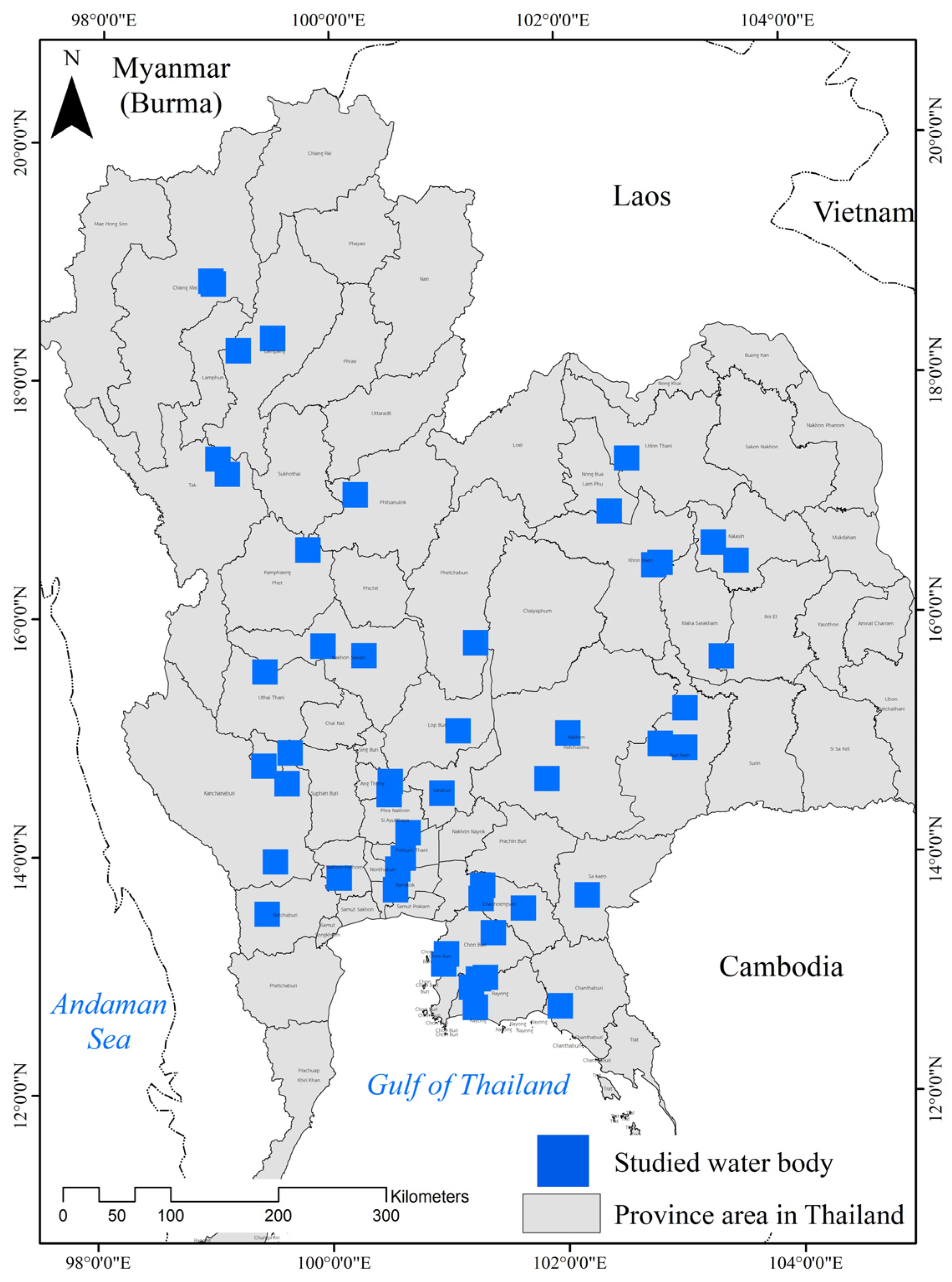
2.1. Study Sites

This study was conducted across 50 lentic water bodies throughout Thailand, classified based on the Trophic State Index (TSI) [18]. It categorized the water bodies as large (a capacity greater than 100 million cubic meters), medium (a capacity of 1–100 million cubic meters), and small (a capacity of less than one million cubic meters) according to the criteria set by Thailand’s Office of the National Water Resources. The sampling campaign was designed to capture variations in trophic status across water bodies of different sizes, depths, and functional uses. The classification criteria also considered water depth and the primary purpose of each water body, such as agricultural use, irrigation, or designation as wetlands of national, international, or global importance under the Ramsar Convention.
A total of nine large water bodies were sampled, with nine sampling stations per site, yielding 81 samples. For the 15 medium-sized water bodies, seven sampling stations were set at each site, resulting in 105 samples. Meanwhile, 26 small water bodies were surveyed, with three stations per site, generating a total of 78 samples. A total of 264 sampling points were distributed across the central, eastern, northeastern, and northern regions of Thailand (Figure 1).

2.2. Field Sampling and Water Quality Analysis

2.2.1. In Situ Water Quality Measurement and Phytoplankton–Zooplankton Sampling

Field surveys and data collection were carried out to evaluate water quality across different trophic gradients. Water, phytoplankton, and zooplankton samples were collected from a range of lentic water bodies exhibiting varying degrees of eutrophication. Sampling was carried out across 50 lentic water bodies between April and May 2024. In situ water quality parameters were measured. Depth (m) was determined using a depth meter, while water temperature (°C) was recorded with a thermo-hygrometer (SK Sato SK-110TRHII Series, Denkei, Schaumburg, IL, USA), which has a temperature accuracy of ±0.5 °C (15–35 °C) and ±1 °C outside this range. pH was measured using a Waterproof pH Testr30 (Cole-Parmer, Vernon Hills, IL, USA), with a high accuracy of ±0.01 pH. Dissolved oxygen (DO, mg/L) was assessed with a HORIBA LAQUAact DO210 Series meter (Horiba, Kyoto, Japan), providing an accuracy of ±0.4 mg/L for concentration. Electrical conductivity (EC, µS/cm) and total dissolved solid (TDS, mg/L) was measured using a COM-101 HM Digital conductivity meter (HM Digital, Carson, CA, USA), with an accuracy within ±2% of the measured value. Water transparency (cm) was evaluated using a Secchi disk, and turbidity (NTU) was measured with a turbidity meter (WTW Turb® 430 IR, Xylem, Washington, DC, USA), with an accuracy of ±2% of the measured value or ±0.01 NTU. Surface water was collected by a 20 L bucket and subsequently filtered through plankton nets with mesh sizes of 22 µm and 64 µm for phytoplankton and zooplankton sampling, respectively. Samples were fixed in 4% formaldehyde and stored at 4 °C for laboratory processing.

2.2.2. Water Quality Analysis and Plankton Study in the Laboratory

Samples for water quality measurements were collected in 1 L bottles for laboratory analysis. Total suspended solids (TSS, mg/L) were measured using the gravimetric method, and chlorophyll-a concentration (µg/L) was analyzed using the acetone extraction method [19]. One-liter water samples for nutrient analysis were preserved by acidifying samples to a pH of <2 with sulfuric acid and stored at 4 °C during transport. Total phosphorus (TP) in µg/L was measured using the Vanadomolybdate method [20]. Total nitrogen (TN) in µg/L was analyzed using a Kjeldahl-type method similar to that described in [20]. Phytoplankton were identified to the genus and species levels and quantified using a Sedgewick-Rafter counting chamber (1.0 mL) under a microscope. Species classification followed the taxonomic guide by Wongrat [21]. For zooplankton, most taxa were also identified to the genus and species levels, except for copepods and ostracods, which were grouped due to limitations in morphological identification. These taxonomic data were then used to calculate various ecological indices.

2.3. Data and Statistical Analyses

The Trophic State Index (TSI) was calculated following the method described by Paulic et al. [18]. First, CHLA (TSI) was calculated using the following formula: CHLA (TSI) = 16.8 + [14.4 × ln (CHLA)]. For calculating nutrient (TSI) or NUTR (TSI), the following limiting nutrient considerations apply: if the ratio of TN/TP is greater than 30, then NUTR (TSI) is equal to TP2 (TSI); if the ratio is less than 10, then NUTR (TSI) is equal to TN2 (TSI); and if the ratio is between 10 and 30, NUTR (TSI) is calculated as the average of TP (TSI) and TN (TSI). TP (TSI) was calculated as TP (TSI) = [18.6 × ln (TP × 1000)] − 18.4, and TP2 (TSI) was calculated as TP2 (TSI) = 10 × [2.36 × ln (TP × 1000)] − 2.38. TN (TSI) was calculated as TN (TSI) = 56 + [19.8 × ln (TN)], and TN2 (TSI) was calculated as TN2 (TSI) = 10 × [5.96 + 2.15 × ln (TN + 0.0001)]. The overall TSI was then derived using the formula: TSI = (CHLA (TSI) + NUTR (TSI))/2. Water bodies were identified as hypereutrophic when the TSI was > 70, as eutrophic when the TSI was 51–70, as mesotrophic when the TSI was 40–50, and as oligotrophic when the TSI was <40.
To assess the overall community diversity, considering both species richness and evenness, the Shannon–Wiener index (Hs) [22], evenness index (E) [23], and species richness index (d) [24] were used to compare phytoplankton and zooplankton diversity across different sites and trophic gradients. The Shannon–Wiener index was calculated using the following formula: Hs = ∑ (pi × ln(pi)), with pi = proportion of the entire community made up of species (i) and E = H/(ln(S)), where S represents species richness. Species richness was further quantified using d = S/√N, where N is the total number of individuals.
To analyze the strength and direction of the associations among water quality parameters and their effects on phytoplankton and zooplankton, correlation analysis was performed using SPSS version 29.0.2.0 (authorized user). A correlation coefficient close to +1 or −1 indicates a strong positive or negative correlation, respectively. Moreover, one-way analysis of variance (ANOVA) and post hoc comparisons (Tukey’s HSD) were performed to evaluate whether the biological indices of phytoplankton and zooplankton differed significantly across different trophic states. Statistically, a p-value of less than 0.05 indicates a statistically significant relationship/difference between groups, whereas a p-value greater than 0.05 indicates no statistically significant effect [25].
A Multidimensional Scaling (MDS) analysis using the software Primer V7 (authorized user) was applied to systematically classify and group water sampling sites. Euclidean distance was used as the similarity measure for the analysis. To address the issue of zero abundance in the dataset, the abundance data were transformed using log(x + 1) prior to the MDS analysis. Datasets with environmental variables (e.g., concentrations of nutrients, temperature, and the abundance of phytoplankton or zooplankton species) were analyzed with Principal Coordinate Analysis (PCoA) [26].

3. Results

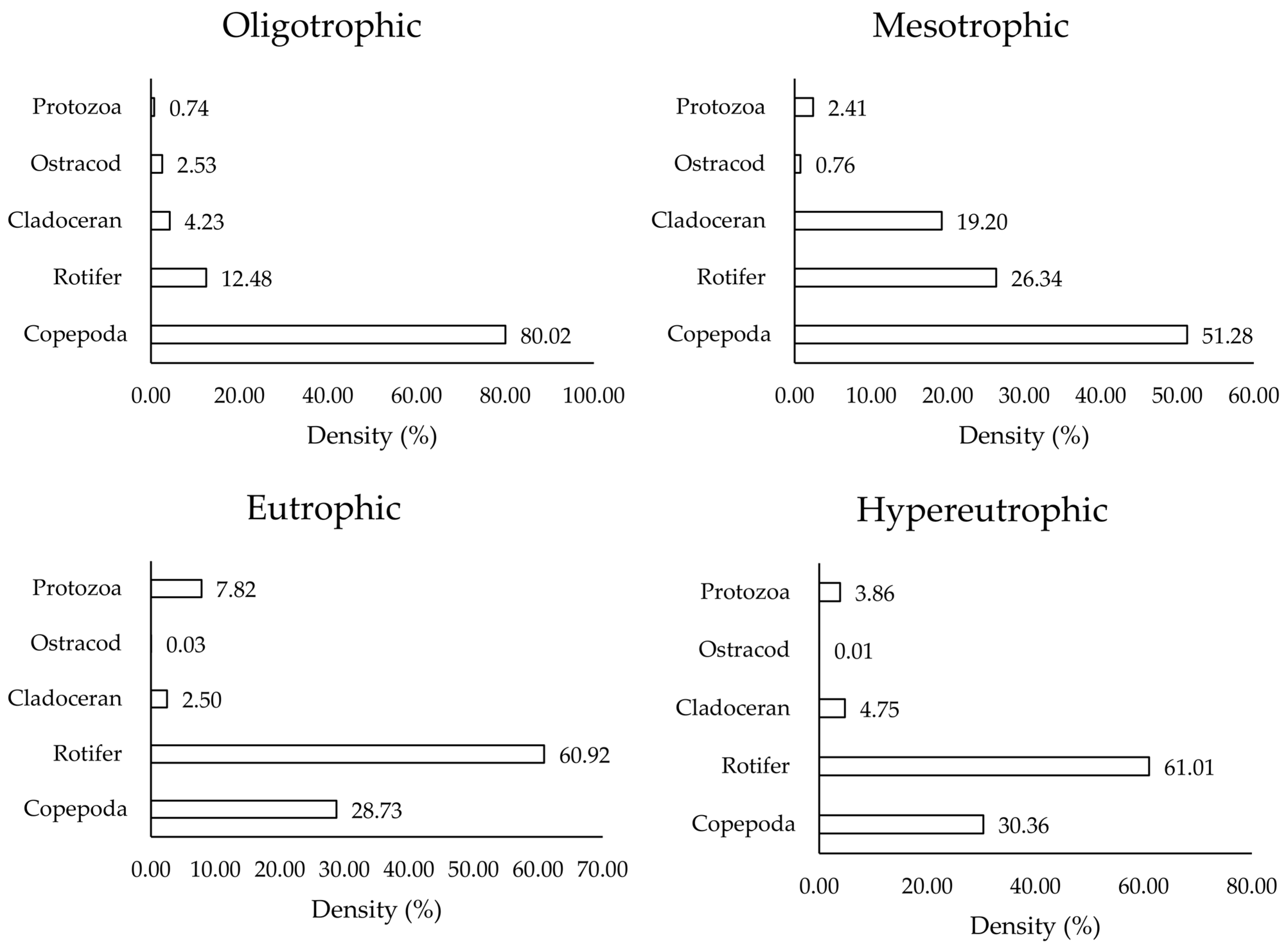
3.1. Phytoplankton and Zooplankton Distribution Across Different Trophic States

A total of 50 sampling sites were classified using the Trophic State Index and showed 26 hypereutrophic water bodies, 17 eutrophic water bodies, six mesotrophic water bodies, and one oligotrophic water body. The average densities of phytoplankton and zooplankton were 22,653 ± 24,358 units/L and 5432 ± 6250 ind./L, respectively.
The distribution of phytoplankton across different trophic statuses of water bodies shows distinct shifts in the dominance of major divisions (Figure 2). In an oligotrophic (nutrient-poor) water body, Dinophyta are the most dominant phytoplankton group, with smaller proportions of Cyanophyta, Chlorophyta, Charophyta, Euglenozoa, Heterokontophyta, and Ochrophyta. In mesotrophic (moderately nutrient-rich) water bodies, Dinophyta remain the leading group, but Charophyta become more prominent, while the presence of Cyanophyta and Chlorophyta declines. As nutrient levels increase to eutrophic conditions, Cyanophyta take over as the dominant division, surpassing Dinophyta, with Euglenozoa and Chlorophyta also becoming more noticeable. In hypereutrophic (highly nutrient-rich) water bodies, Cyanophyta clearly dominate, followed by Euglenozoa and Chlorophyta, whereas Dinophyta play a much smaller role. Overall, the trend shows a decline in Dinophyta dominance and a significant increase in Cyanophyta prevalence as nutrient levels in water bodies rise. Other groups, such as Euglenozoa and Chlorophyta, vary in abundance depending on the trophic status.
The composition of zooplankton varies noticeably according to the trophic status of water bodies (Figure 3). In an oligotrophic water, Copepoda are the most dominant zooplankton group, followed by Rotifers, while other groups like Cladocerans, Ostracods, and Protozoa are present in smaller proportions. In mesotrophic waters, Copepoda continue to be dominant, but the presence of Rotifers and Cladocerans becomes more prominent, showing a more balanced composition. As nutrient levels rise in eutrophic waters, Rotifers overtake Copepoda as the dominant group, while Protozoa increase in abundance, and Cladocerans and Ostracods decline. In hypereutrophic conditions, Rotifers remain the most dominant group, followed by Copepoda, while Cladocerans, Protozoa, and Ostracods appear only in smaller amounts. Overall, the trend shows a shift in dominance from Copepoda to Rotifers as water bodies become more nutrient-rich, with other groups adjusting their presence according to the changing environment.

3.2. Dominant Phytoplankton and Zooplankton Species

This study identifies the dominant phytoplankton and zooplankton species in lentic water bodies across different trophic states, along with their respective phyla and population densities. For phytoplankton, Peridinium sp. of the phylum Dinophyta is the dominant species in both oligotrophic and mesotrophic waters, with densities of 1836 units/L and 18,424 ± 20,625 units/L, respectively. As trophic levels rise to eutrophic and hypereutrophic states, Oscillatoria sp. from the phylum Cyanophyta becomes dominant, with Cyanophyta showing the highest abundance at 17,777 ± 19,365 units/L and 19,539 ± 18,953 units/L, respectively. Copepods, belonging to the phylum Arthropoda, subphylum Crustacea, and class Copepoda, dominate the zooplankton community in oligotrophic and mesotrophic water bodies. Their densities range from 2591 ind./L in oligotrophic water to 2283 ± 1577 ind./L in hypereutrophic waters. In contrast, Rotifers were the dominant group in eutrophic and hypereutrophic water bodies, reflecting their adaptability to nutrient-rich conditions. Rotifer densities in eutrophic and hypereutrophic water bodies were 3523 ± 6855 ind./L and 3581 ± 4374 ind./L, respectively.

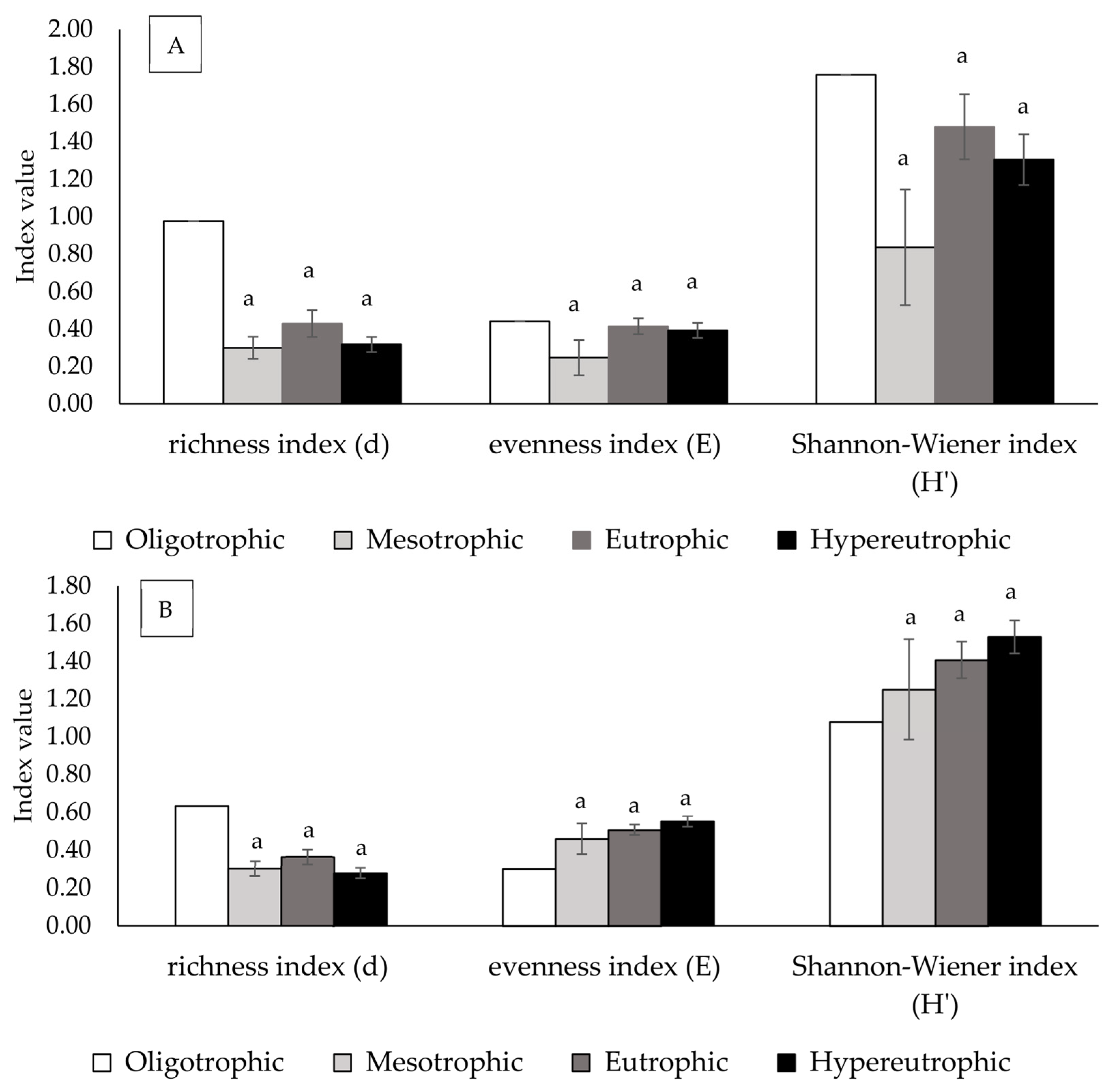
3.3. Effects of Trophic Status on Phytoplankton and Zooplankton Richness, Evenness, and Shannon-Wiener Indices

Phytoplankton richness index was the highest (0.98) in an oligotrophic water body and was the lowest (0.32 ± 0.04) in hypereutrophic water bodies (Figure 4A). The Shannon–Wiener index shows a similar trend, with a peak of 1.76 in oligotrophic and a minimum in mesotrophic waters (0.84 ± 0.31). Similarly, the evenness index is the highest in an oligotrophic water (0.44), whereas it is the lowest (0.25 ± 0.09) in mesotrophic waters. Figure 4B shows comparable results for zooplankton. The richness index is the highest in the oligotrophic water body (0.63) and the lowest in hypereutrophic waters (0.28 ± 0.03). Contrarily, Shannon–Wiener and evenness indices indicated an opposite trend with minimum values in oligotrophic water (1.08 and 0.30, respectively), while the highest values were observed in hypereutrophic waters (1.5 ± 0.09 and 0.56 ± 0.03, respectively).

3.4. Assessing the Relationship Between Water Quality, Phytoplankton, and Zooplankton Using Correlation Analysis

The densities of both phytoplankton and zooplankton were markedly positively correlated with certain water quality parameters, reflecting their unique environmental preferences (Table 1). Pearson’s correlation coefficient was used to analyze these relationships. For the phytoplankton, the Cyanophyta groups displayed significant positive correlations with TDS (r = 0.383, p < 0.01) and EC (r = 0.403, p < 0.01). Chlorophyta were positively correlated with TN (r = 0.456, p < 0.01) and TP (r = 0.317, p < 0.05). In contrast, Dinophyta showed positive correlations with DO (r = 0.319, p < 0.05) and Secchi depth (r = 0.317, p < 0.05). For zooplankton, Rotifers were significantly positively correlated with TP (r = 0.358, p < 0.05), TDS (r = 0.387, p < 0.01), and EC (r = 0.422, p < 0.01). Ostracods were significantly correlated with Secchi depth (r = 0.496, p < 0.01).

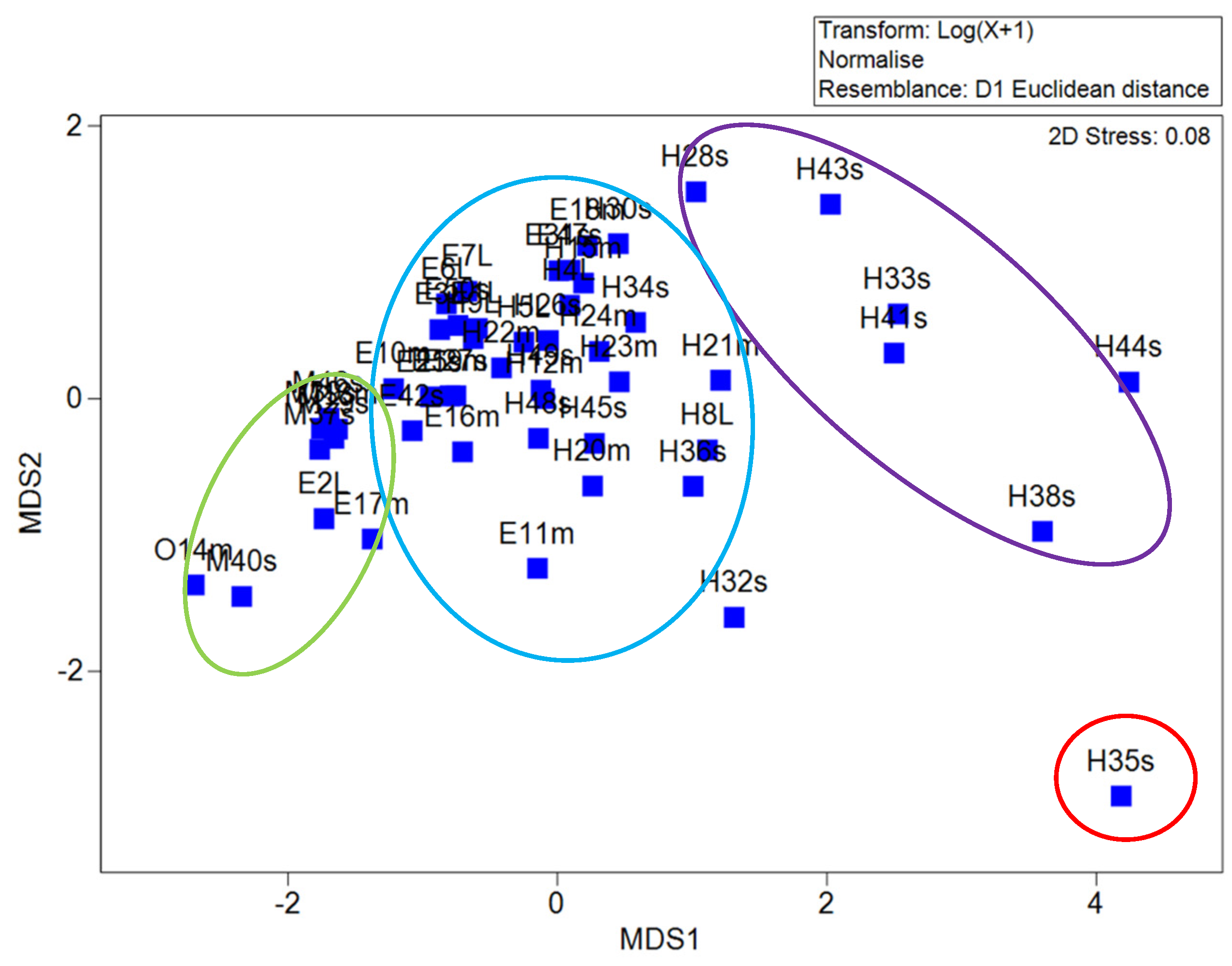
3.5. Multidimensional Scaling Analysis

Figure 5 presents a Multidimensional Scaling analysis of 50 water bodies, illustrating similarities and differences in environmental variables across various locations. The plot reveals distinct clusters of water bodies, highlighted with blue, green, and purple circles, indicating that water bodies within the same cluster share similar water quality traits, while those in different clusters exhibit significant differences. H35s, a small hypereutrophic water body (marked with red circles), is clearly distinct from all other water bodies, suggesting a significant deviation in water quality. This separation can be attributed to factors such as pollution, unique chemical composition, and site-specific activities, which may collectively influence the water quality of this particular site.

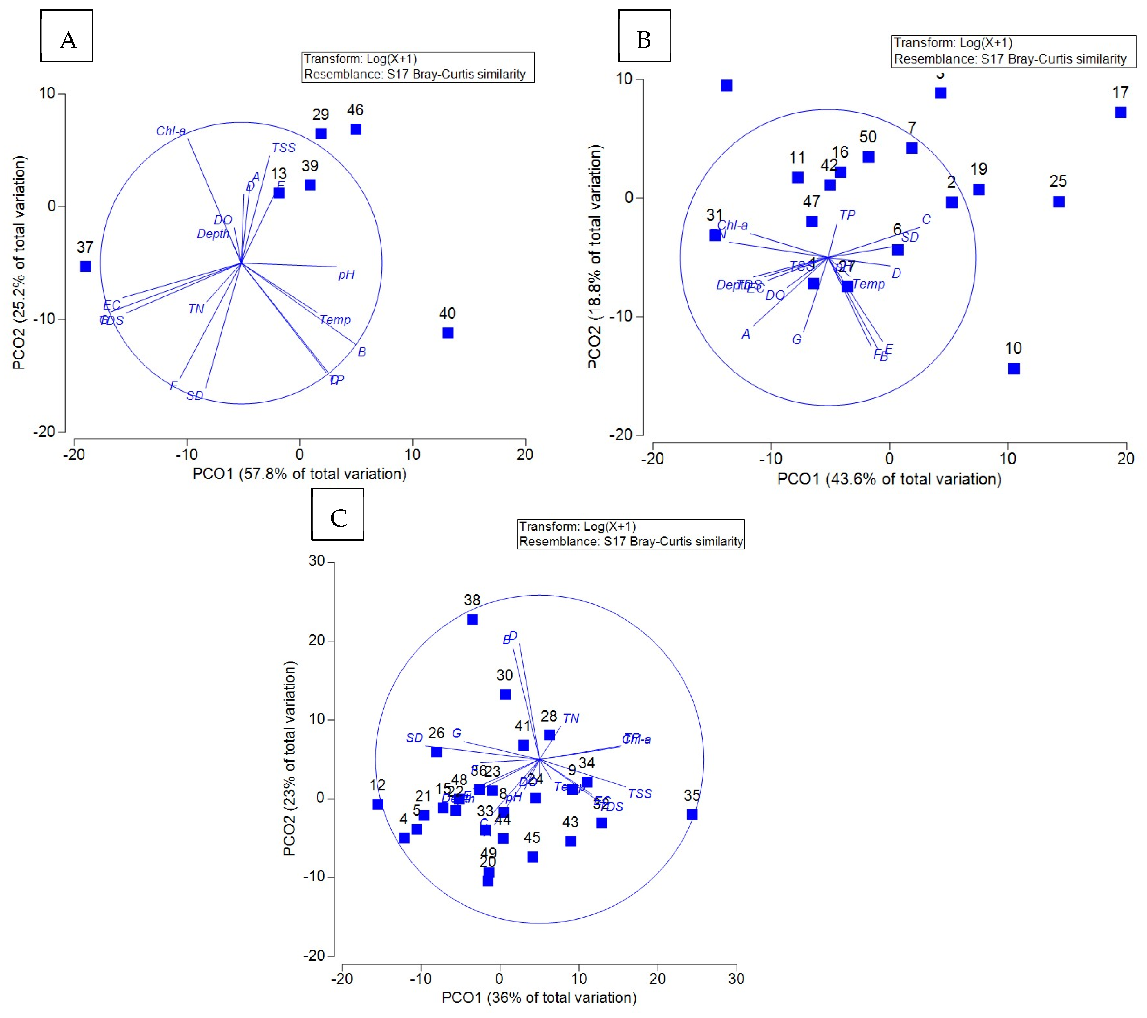
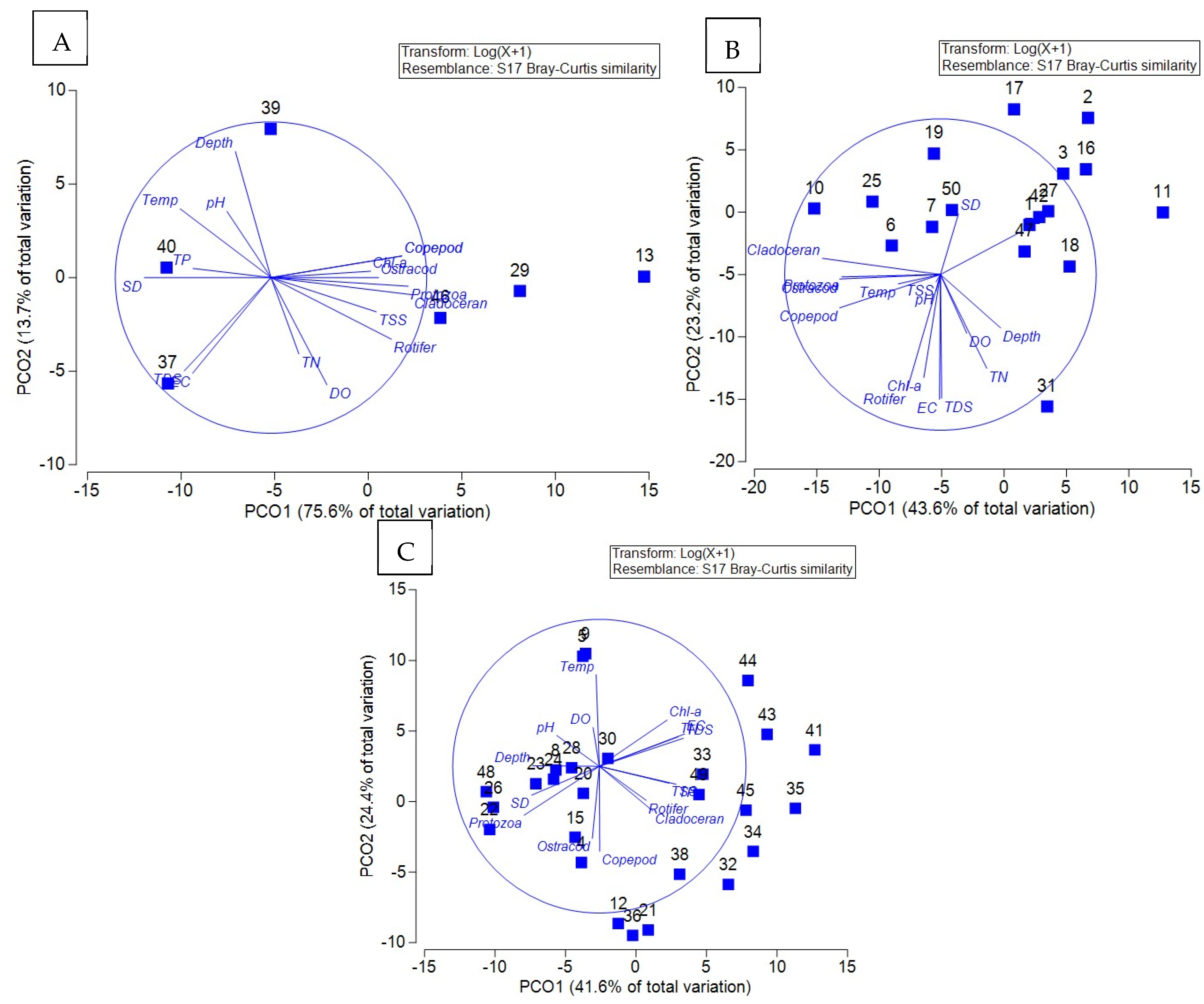
3.6. Principal Coordinate Analysis of the Relationship Between Water Quality and Plankton Communities in Trophic Water Bodies

The Principal Coordinate Analysis diagrams show the relationships between phytoplankton and water quality variables for each trophic level. In this study, only one oligotrophic site was available, resulting in insufficient data for PcoA. In the mesotrophic water bodies (Figure 6A), phytoplankton groups such as Euglenozoa, Dinophyta, Ochrophyta, and Chlorophyta were generally influenced by TDS, EC, chlorophyll-a, TN, and TP. Some sampling points—specifically 37, 40 and 46—exhibited distinct water quality characteristics. In the eutrophic water bodies (Figure 6B), higher concentrations of nutrients were observed, and the phytoplankton community structure was primarily associated with the elevated levels of TSS, TP, and TN. Notably, sites 10, 17, and 25 deviated from the overall pattern. In the hypereutrophic water body (Figure 6C), Dinophyta, Ochrophyta, Chlorophyta, and Euglenozoa are associated with water transparency, while other groups are representative of nutrient content levels.
Figure 7A presents a PCoA illustrating the relationships between zooplankton communities and water quality variables. In mesotrophic water bodies, TN, TP, and TSS were closely associated with Rotifers, Cladocerans, Copepoda, and Protozoa, whereas Ostracods exhibited a distinct response pattern. For example, 29 and 46 exhibit similar water quality and zooplankton composition, while 37, 39, and 40, positioned farther from the center, may reflect markedly different water quality conditions or zooplankton assemblages. As demonstrated in Figure 7B,C, PCoA shows a positive correlation between TDS, TSS, TP, and major zooplankton groups like Rotifers and Copepoda, suited to nutrient-rich conditions. Ostracod, Protozoa, and Cladoceran show an opposite trend, suggesting a weaker association.

4. Discussion

4.1. Phytoplankton and Zooplankton Distribution Across Different Trophic States

This study contributes to understanding the health of the sampled water bodies across different trophic states and their impact on plankton populations in tropical environments. The study was conducted during the summer season because this period represents the most ecologically dynamic phase in tropical lentic water bodies. Higher temperatures and low water levels during this time intensify nutrient concentrations and biological activity, allowing clearer detection of trophic gradients and planktonic responses.
Phytoplankton community composition shifts noticeably along the trophic gradient. Peridinium sp. (Dinophyta) is the dominant phytoplankton in oligotrophic and mesotrophic water bodies, indicating that these habitats maintain relatively stable and moderate nutrient conditions conducive to dinoflagellate populations. Dinoflagellates, typically associated with stable waters, imply a better water quality compared to the highly eutrophic sites [27]. This is consistent with observations from several Thai reservoirs, including Kaeng Krachan Reservoir and Mae Suai Reservoir, where Peridinium sp. was found to dominate during periods of moderate nutrient levels and stratified water columns [28,29]. Moreover, the increase in Charophyta species, which prefer pristine, low-nutrient waters, indicates improving ecological conditions. However, as nutrient enrichment from agricultural runoff, sewage discharge, and other anthropogenic activities increases [30], Cyanophyta become dominant in eutrophic and hyper-eutrophic conditions. Cyanophyta have various physiological adaptations that give the taxa competitive advantages in nutrient-laden and stratified water [31]. Traits such as nitrogen fixation, buoyancy regulation, and the ability to store phosphate internally as polyphosphate granules enable Cyanophyta to thrive and establish dominance in these environments [32]. When resources are abundant, cyanobacteria can outcompete other phytoplankton [33]. In this study, Oscillatoria sp. has high densities and dominates specific ecosystems, indicating a higher risk of cyanobacterial blooms with detrimental ecological and water quality impacts [34].
The zooplankton community structure changes significantly with the trophic status, as this is directly proportional to changes in nutrient abundance and environmental conditions. Protozoa and ostracods were consistently observed at lower densities than other zooplankton groups across all trophic conditions. This may be attributed to their smaller size, lower reproductive rates and limited adaptability to fluctuating nutrient levels [35,36]. Ostracods were more abundant in oligotrophic conditions, indicating a preference for clearer, low-nutrient waters [37,38], whereas Cladocerans reached their highest densities in mesotrophic conditions and act as key grazers, helping to control phytoplankton populations and enhance water clarity and ecosystem stability [39]. We also observe a clear change in oligotrophic and mesotrophic water bodies when the Copepoda group is predominant, and the Rotifer density drops significantly [40]. Such a shift indicates better water quality and a healthier ecosystem, since Copepoda and Cladocerans are often related to regulated trophic interactions and less organic pollution [41]. Nonetheless, the lower Copepoda densities in hypereutrophic waters could hint increased competition, heightened predation pressure, or reduced water quality [42]. Meanwhile, Rotifers are most concentrated in eutrophic and hypereutrophic waters, representing the high availability of organic matter and small-sized phytoplankton, which are their main diet. Their strong presence in nutrient-rich environments supports previous findings indicating that Rotifers are highly tolerant of eutrophic conditions and thrive in ecosystems with elevated bacterial and algal biomass [39]. Similarly, a Thai study on the seasonal variation of zooplankton assemblages and their responses to water chemistry and microcystin content in shallow lakes reported Rotifers and Copepoda as the dominant group under nutrient-rich conditions [39]. In addition, a prior freshwater study showed that Rotifers exhibited the highest species richness among all zooplankton taxa [43].
Although our results highlight the complex relationships between nutrient availability and plankton community composition [44], a limitation of this study is its single-season data collection, which may not fully reflect the seasonal variations in plankton communities and environmental conditions. Future research should address this limitation and also consider other biological (e.g., zooplanktivorous fishes) and chemical parameters (e.g., heavy metals and synthetic compounds) that may influence the plankton community structure.

4.2. Phytoplankton and Zooplankton Richness, Evenness, and Shannon–Wiener Indices Among Water Bodies Across Different Trophic States

According to this study, phytoplankton diversity tends to peak in an oligotrophic water body but declines with the increasing levels of nutrients, reaching its lowest under hypereutrophic conditions. This trend fits with ecologists’ understanding that, in low-nutrient water bodies, competition is weak among the phytoplankton species, and this allows more species to coexist. However, when the nutrient levels become excessive [45], highly nutrient-efficient species, including the cyanobacterial genera, dominate the system by blocking light and producing toxins that inhibit other organisms and reduce overall biodiversity [46]. In mesotrophic waters, which contain moderate levels of nutrients, a more balanced and diverse phytoplankton community is supported; however, slight imbalances may develop as competitive species increase in prevalence. Higher nutrient efficiency and deeper light penetration allow several species to co-occur, thereby maintaining the ecological stability [47].
On the other hand, zooplankton displays a reverse pattern: the highest Shannon–Wiener and evenness indices are seen in hypereutrophic waters, while oligotrophic waters have the lowest values. These trends might relate to the fact that zooplankton communities are closely controlled by phytoplankton composition and organic matter concentrations [48]. Thus, only a few adapted species can survive in oligotrophic waters with insufficient nutrients, while high-nutrient waters usually have a diverse community of zooplankton due to the abundant supply of food. However, in some situations, excessive phytoplankton growth, especially of cyanobacterial species, can exert a negative impact on the zooplankton community structure [49]. This inconsistency suggests that, although higher nutrient levels generally support greater zooplankton diversity, the degraded food quality and environmental conditions associated with the onset of eutrophic or hypereutrophic states may instead lead to reduced diversity, contrary to findings from some previous studies.

4.3. The Relationship Between Water Quality, Phytoplankton, and Zooplankton

The distribution of phytoplankton is governed by the availability of nutrients and physical and chemical factors. Cyanophyta (blue-green algae) were positively correlated only with TDS and EC [50], indicating their success in lakes with high ionic content or those rich in nutrients. Such conditions are typical of eutrophic and hypertrophic water bodies. Chlorophyta (green algae) were also largely dependent on nutrient inputs, with TN and TP showing a significant positive correlation with their biomass. This result aligns with previous findings, as Chlorophyta are known to proliferate rapidly in nitrogen- and phosphorus-enriched waters [51], particularly in mesotrophic-to-eutrophic environments. Dinophyta were positively correlated with DO and Secchi depth, suggesting this group prefers well-oxygenated, clearer water [52]. Dinophyta were not entirely absent; instead, they flourished in water bodies with ideal light conditions, as these organisms reside in water bodies with high Secchi depth values.
Zooplankton are central to aquatic food webs, connecting primary producers (e.g., phytoplankton) to higher trophic levels. Their distribution and presence are highly dependent on the water quality conditions. Increases in TP, TDS, and EC were highly correlated (positively) with the presence of Rotifers, thus suggesting that Rotifers are commonly found in nutrient-rich waters with greater ionic concentrations [53]. They can multiply quickly, enabling them to directly respond to rising nutrient levels; thus, they are considered good bioindicators of water quality changes [54]. Ostracods exhibit a high positive correlation with Secchi depth, indicating that they prefer clearer waters. Indeed, their benthic or aquatic plant-associated lifestyle [37] may be linked to this preference, since many ostracod species are sediment or aquatic vegetation residents, which have the best growth potential in relatively clear waters [38]. The association of ostracods with clear waters suggests that they are more likely to be associated with stable aquatic environments, while Rotifers tend to be favored by more disturbed, nutrient-rich waters. This contrast is consistent with the different habitat preferences of the zooplankton groups.

4.4. Analysis of Multidimensional Scaling and Principal Coordinate Analysis

These 50 studied water bodies cluster within neighboring polygons, as shown with the MDS analysis, in which polygons were plotted based on the similarity and dissimilarity of water quality. As displayed in the MDS plot, the water bodies within each group (depicted in blue, green, and purple circles) form clusters, indicating that their water quality characteristics are similar. The green-circled group comprises oligo-mesotrophic water bodies characterized by low nutrient (TN, TP) and chlorophyll-a levels, high transparency, and low-moderate plankton densities. The blue-circled group represents water bodies with intermediate values across these parameters. In contrast, the purple-circled group includes hypereutrophic water bodies with high nutrient and chlorophyll-a levels, low transparency, and dense phytoplankton populations. In addition, H35s (a small hypereutrophic water body) is clearly separated from the other water bodies due to a significant difference in water quality compared to the rest. H35s refers to Bueng Thung Sang, located in Khon Kaen Province, Northeastern Thailand. This water body exhibits an exceptionally low density of phytoplankton, with only 735 units/L, while zooplankton are present in large numbers, with a density of 23,114 ind./L. This atypical biological composition is likely one of the primary factors that distinguish this site from others, as, in most locations, phytoplankton density typically surpasses that of zooplankton [55].
The overall trends from PCoA suggest a different response for phytoplankton and zooplankton communities across trophic levels, likely driven by nutrient availability, suspended solids, and light. In contrast, clear changes are observed in dominant environmental drivers and biological assemblages with an increasing trophic state extending from mesotrophic to hypereutrophic water bodies [56]. In eutrophic and hypereutrophic water bodies, the relationships of phytoplankton were predominantly influenced by nutrients and TSS, particularly affecting phytoplankton structure and promoting some zooplankton like Rotifers and Copepoda [57,58].

5. Conclusions

The trophic status of lentic water bodies plays a fundamental role in shaping plankton structure and abundance in Thailand. Hypereutrophic waters exhibited the highest phytoplankton density, primarily dominated by Cyanophyta, whereas oligotrophic waters supported the greatest species richness and were characterized by the prevalence of Dinophyta. Rotifers and Copepoda were the more abundant plankton in nutrient-rich conditions, while zooplankton diversity peaked in mesotrophic and oligotrophic ecosystems. As a case study from a tropical region, this research provides foundational data for cross-regional comparison, contributing valuable insights into ecological responses under varying nutrient regimes. The statistically supported relationships between environmental parameters and plankton communities underscore the utility of these organisms as practical bioindicators for tropical freshwater systems. This framework offers water managers a science-based tool for assessing eutrophication trends and ecosystem health. We recommend that future research prioritize long-term, multi-seasonal datasets and incorporate the functional traits of plankton to improve the precision and applicability of bioindicator systems across trophic gradients.

Author Contributions

Conceptualization, P.P., R.C., C.R., P.K., W.C. and S.M.; Methodology, P.P., R.C., C.R., P.K., W.C. and S.M.; Formal Analysis, P.P., R.C., C.R., P.K., W.C. and S.M.; Investigation, P.P. and R.C.; Data Collection, P.P., R.C., C.R. and S.M.; Writing—Original Draft Preparation, P.P. and R.C.; Writing—Review and Editing, R.C., C.R., P.K., W.C. and S.M.; Visualization, R.C., P.K., W.C. and S.M.; Supervision, R.C., P.K., W.C. and S.M. All authors have read and agreed to the published version of the manuscript. published version of the manuscript.

Funding

National Research Council of Thailand (NRCT): N25A670665.

Institutional Review Board Statement

The animal study protocol was approved by the Animal Ethics Committee of Kasetsart University (Approval No. ACKU68-ETC-006, approved on 13 May 2025).

Data Availability Statement

Data contained within the article.

Acknowledgments

This research was financially supported by the National Research Council of Thailand (NRCT) under the Ministry of Higher Education, Science, Research, and Innovation (MHESI) through the Research and Innovation Fund for Natural Resources and Environment for the Fiscal Year 2024 (N25A670665), under the topic ‘Marine and Coastal Ecosystems and Blue Economy’.

Conflicts of Interest

The authors declare no conflict of interest.

References

  1. Antonati, M.; Poikane, S.; Pringle, C.; Stevens, L.; Turak, E.; Heino, J.; Richardson, J.; Bolpagni, R.; Borrini, A.; Cid, N.; et al. Characteristics, main impacts, and stewardship of natural and artificial freshwater environments: Consequences for biodiversity conservation. Water 2020, 12, 260. [Google Scholar] [CrossRef]
  2. Bobacina, L.; Fasano, F.; Mezzanotte, V.; Fornaroli, R. Effects of water temperature on freshwater macroinvertebrates: A systematic review. Biol. Rev. Camb. Philos. Soc. 2023, 98, 191–221. [Google Scholar] [CrossRef] [PubMed]
  3. Wijewardene, L.; Wu, N.; Qu, Y.; Guo, K.; Messyasz, B.; Lorenz, S.; Riis, T.; Ulrich, U.; Fohrer, N. Influences of pesticides, nutrient, and local environmental variables on phytoplankton communities in lentic small water bodies in German lowland agricultural area. J. Sci. Total Environ. 2021, 780, 146481. [Google Scholar] [CrossRef]
  4. Aktar, M.W.; Sengupta, D.; Chowdhury, A. Impact of pesticides use in agriculture: Their benefits and hazards. Interdiscip. Toxicol. 2009, 2, 1–12. [Google Scholar] [CrossRef]
  5. Soininen, J.; Luoto, M. Is catchment productivity a useful predictor of taxa richness in lake plankton communities? Ecol. Appl. 2012, 22, 624–633. [Google Scholar] [CrossRef]
  6. Florescu, L.I.; Moldoveanu, M.M.; Catana, R.D.; Pacesila, I.; Dumitrache, A.; Gavrilidis, A.A.; Ioja, C.I. Assessing the effects of phytoplankton structure on zooplankton communities in different types of urban lakes. Diversity 2022, 14, 231. [Google Scholar] [CrossRef]
  7. Ochocka, A.; Pasztaleniec, A. Sensitivity of plankton indices to lake trophic conditions. Environ. Monit. Assess. 2016, 188, 622. [Google Scholar] [CrossRef]
  8. Stamou, G.; Katsiapi, M.; Moustaka-Gouni, M.; Michaloudi, E. Trophic state assessment based on zooplankton communities in Mediterranean lakes. Hydrobiologi 2019, 844, 83–103. [Google Scholar] [CrossRef]
  9. Kovalenko, K.E.; Reavie, E.D.; Figary, S.; Rudstam, L.G.; Watkins, J.M.; Scofield, A.; Filstrup, C.T. Zooplankton-phytoplankton biomass and diversity relationship in the Great Lakes. PLoS ONE 2023, 18, e0292988. [Google Scholar] [CrossRef]
  10. Dodds, W.K.; Smith, V.H. Nitrogen, phosphorus, and eutrophication in streams. Inland Waters 2016, 6, 155–164. [Google Scholar] [CrossRef]
  11. Ho, J.C.; Michalak, A.M.; Pahlevan, N. Widespread global increase in intense lake phytoplankton blooms since the 1980s. Nature 2019, 574, 667–670. [Google Scholar] [CrossRef] [PubMed]
  12. Elser, J.J.; Goldman, C.R. Zooplankton effects on phytoplankton in lakes of contrasting trophic status. Am. Soc. Limnol. Oceanogr. 1991, 36, 64–90. [Google Scholar] [CrossRef]
  13. Ekvall, M.K.; Urrutia-Cordero, P.; Hansson, L. Linking cascading effects of fish predation and zooplankton grazing to reduced Cyanobacterial biomass and toxin levels following biomanipulation. PLoS ONE 2014, 9, e112956. [Google Scholar] [CrossRef]
  14. Anuttarunggoon, N.; Anurakpongsatorn, P.; Tantanasarit, S.; Mahujchariyawong, J. Characterization of water quality in Bunboraped wetland, Thailand using self organizing map for water quality management. EnvironmentAsia 2020, 13, 114–123. [Google Scholar]
  15. Singkran, N. Determining overall water quality related to anthropogenic influences across freshwater systems of Thailand. Water Resour. Dev. 2017, 33, 132–151. [Google Scholar] [CrossRef]
  16. Prasertphon, R.; Jitchum, P.; Chaichana, R. Water chemistry, phytoplankton diversity and severe eutrophication with detection of Microcystin contents in Thai tropical urban ponds. Ecol. Environ. Res. 2020, 18, 5939–5951. [Google Scholar] [CrossRef]
  17. Descy, J.-P.; Leprieur, F.; Pirlot, S.; Leporcq, B.; Van Wichelen, L.; Peretyatko, A.; Teissier, S.; Codd, G.A.; Triest, L.; Vyverman, W.; et al. Identifying the factor determining blooms of cyanobacteria in a set of shallow lakes. Ecol. Inform. 2016, 34, 129–138. [Google Scholar] [CrossRef]
  18. Paulic, M.; Hand, J.; Lord, L. Water-Quality Assessment for the State of Florida Section 305(B) Main Report; Bureau of Water Resources Protection: Tallahassee, FL, USA, 1996; p. 317. [Google Scholar]
  19. Talling, J.F.; Driver, D. Some problems in the estimation of chlorophyll-a in phytoplankton. In Proceedings of the Conference of Primary Productivity Measurement, Marine and Freshwater, Honolulu, HA, USA, 21 August–6 September 1961; Atomic Energy Commission: Washington, DC, USA, 1963; pp. 142–146. [Google Scholar]
  20. American Public Health Association; American Water Works Association; Water Environment Federation. Standard Methods for the Examination of Water and Wastewater; American Public Health Association: Washington, DC, USA, 2017. [Google Scholar]
  21. Wongrat, L.; Wongrat, P.; Ruangsomboon, S. Plankton; Faculty of Fisheries, Kasetsart University: Bangkok, Thailand, 1987. [Google Scholar]
  22. Shannon, C.E. A Mathematical Theory of Communication. Bell Syst. Tech. J. 1948, 27, 379–423. [Google Scholar] [CrossRef]
  23. Pielou, C.E. The measurement of biodiversity in different types of biological collections. J. Theor. Biol. 1966, 13, 131–144. [Google Scholar] [CrossRef]
  24. Menhinick, E.F. A comparison of some species-individuals diversity indices applied to samples of field insects. Ecology 1964, 45, 859–861. [Google Scholar] [CrossRef]
  25. SPSS About SPSS Inc. Available online: http://www.spss.com.hk/corpinfo/history.htm (accessed on 1 April 2025).
  26. Clarke, K.R.; Gorley, R.N. PRIMER v7: User Manual/Tutorial; PRIMER-E Ltd.: Devon, UK, 2015; 296p. [Google Scholar]
  27. Nasution, A.K.; Takarina, N.D.; Thoha, H. The presence and abundance of harmful dinoflagellate alae related to water quality in Jakarta Bay, Indonesia. Biodiversitas 2021, 22, 2909–2917. [Google Scholar] [CrossRef]
  28. Meesukko, C.; GaJaswni, N.; Peerapornpisal, Y.; Voinov, A. Relationships between seasonal variation and phytoplankton dynamics in Kaeng Krachan reservoir, Phetchaburi province, Thailand. Nat. Hist. J. Chulalongkorn Univ. 2007, 7, 131–143. [Google Scholar] [CrossRef]
  29. Prasertsin, T.; Yavichai, S.; Pingmano, C. Diversity of phytoplankton and water quality in Mae Suai reservoir during the rainy season. Prog. Appl. Sci. Tech. 2025, 8, 184–199. [Google Scholar]
  30. Rahman, R.M.; Greco, A.; Nanda, A.; Rios-Ruiz, C.; Wang, Y.; Yoon, P.; Restaina, D.J.; Gaynor, J.J.; Bologna, P.A.X.; Chu, T. Detection and characterization of the Cyanobacteria and Cyanophages of Barnegat Bay, New Jersey. J. Environ. Prot. 2019, 10, 1472–1483. [Google Scholar] [CrossRef]
  31. Wang, W.; He, Z.; Lv, J.; Liu, X.; Xie, S.; Feng, J. Cyanobacteria as dominant mediator of altitudinal gradient effects on phytoplankton community diversity in freshwater ecosystems: Evidences from the freshwater Lakes along the Hu Line. Water Res. X 2025, 26, 100281. [Google Scholar] [CrossRef]
  32. San-Luque, E.; Bhaya, D.; Grossman, A.R. Polyphosphate: A multifunctional metabolite in Cyanobacteria and algae. Front. Plant Sci. 2020, 11, 938. [Google Scholar]
  33. Hessen, D.O.; Faafeng, B.A.; Brettum, P.; Andersen, T. Nutrient enrichment and planktonic biomass ratios in lakes. Ecosystems 2006, 9, 516–527. [Google Scholar] [CrossRef]
  34. Weisse, T.; Gröschl, B.; Bergkemper, V. Phytoplankton response to short-term temperature and nutrient changes. Limnologica 2016, 59, 78–89. [Google Scholar] [CrossRef]
  35. Yousef, E.A.; El-Mallah, A.M.; Abdel-Baki, A.-A.S.; Al-Quraishy, S.; Reyad, A.; Abdel-Tawab, H. Effect of environmental variables on zooplankton in various habitats of the Nile River. Water 2024, 16, 915. [Google Scholar] [CrossRef]
  36. Mansano, A.S.; Hisatugo, K.F.; Leite, M.A.; Regali-Seleghim, M.H. Seasonal variation of the protozooplanktonic community in a tropical oligotrophic environment (Ilha Solteira reservoir, Brazil). Braz. J. Biol. 2013, 73, 321–330. [Google Scholar] [CrossRef]
  37. Külköylüoglu, O.; Sari, N.; Dügel, M.; Dere, S.; Dalkiran, N.; Aygen, C.; Dincer, C. Effects of limnoecological changes on the Ostracoda (Crustacea)community in a shallow lake (Lake Çubuk, Turkey). Limnologica 2014, 46, 99–108. [Google Scholar] [CrossRef]
  38. Kolarova, N.; Napiórkowski, P. Are rotifer indices suitable for assessing the trophic status in slow-flowing waters of canals. Hydrobiologia 2024, 851, 3013–3023. [Google Scholar] [CrossRef]
  39. Pransertphon, R.; Chaichana, R.; Jitchum, P. Seasonal variation of zooplankton assemblages and their response to water chemistry and microcystin content in shollow lakes in Thaland. Arch. Biol. Sci. 2023, 75, 369–378. [Google Scholar] [CrossRef]
  40. Paturej, E.; Kowalska, E. Rotifers trophic state indices as ecosystem indicators in Brackish coastal waters. Oceanologia 2013, 55, 887–889. [Google Scholar]
  41. Umi, W.A.D.; Yusoff, F.M.; Yusof, Z.N.B.; Ramli, N.M.; Sinev, A.Y.; Toda, T. Composition, distribution, and biodiversity of zooplanktons in tropical lentic ecosystems with different environmental conditions. Arthropoda 2024, 2, 33–54. [Google Scholar] [CrossRef]
  42. Hogfors, H.; Motwani, N.H.; Haidu, S.; El-Shehawy, R.; Holmborn, T.; Vehmaa, A.; Engström-öst, J.; Bretemark, A.; Gorokhova, E. Bloo-forming cyanobacteria support copepoda reproduction and development in the Baltic Sea. PLoS ONE 2014, 9, e112692. [Google Scholar] [CrossRef]
  43. Cabral, C.R.; Diniz, L.P.; da Silva, A.J.; Fonseca, G.; Carneiro, L.S.; de Melo Junior, M.; Caliman, A. Zooplankton species distribution, richness and composition across tropical shallow lakes: A large scale assessment by biome, lake origin, and lake habitat. Ann. Limnol. Int. J. Lim. 2020, 56, 25. [Google Scholar] [CrossRef]
  44. Nes, E.H.V.; Scheffer, M.; Berg, M.S.V.D.; Coops, H. Dominance of charophytes in eutrophic shallow lakes-When should we expect it to be an alternative stable state? Aquat. Bot. 2002, 72, 275–296. [Google Scholar]
  45. Alvarez, E.; Lazzari, P.; Cossarini, G. Phytoplankton diversity emerging from chromatic adaptation and competition for light. Prog. Oceanogr. 2022, 204, 102789. [Google Scholar] [CrossRef]
  46. Lehtinen, S.; Tamminen, T.; Ptacnik, R.; Andersen, T. Phytoplankton species richness, evenness, and production in relation to nutrient availability and imbalance. Limnol. Oceanogr. 2017, 62, 1393–1408. [Google Scholar] [CrossRef]
  47. Kardinaal, W.E.A.; Tonk, L.; Janse, I.; Hol, S.; Slot, P.; Huisman, J.; Visser, P.M. Competition for light between toxic and nontoxic strains of the harmful cyanobacterium Microcystis. Appl. Environ. Microbiol. 2007, 73, 2939–2946. [Google Scholar] [CrossRef] [PubMed]
  48. Perbiche-Neves, G.; Saito, V.S.; Previattelli, D.; Rocha, C.E.F. Cyclopoid copepoda as bioindicators of eutrophication in reservoirs: Do patterns hold for large spatial extents. Ecol. Indic. 2016, 70, 340–347. [Google Scholar] [CrossRef]
  49. Kuczyn’ska-Kippen, N.; Joniak, T. Zooplankton diversity and macrophyte biometry in shallow water bodies of various trophic state. Hydrobiologia 2016, 774, 39–51. [Google Scholar] [CrossRef]
  50. Kalinowska, K.; Napiórkowska-Krzebietke, A.; Bogacka-Kapusta, E.; Stawecki, K.; Traczuk, P.; Ulikowski, D. Algae-zooplankton relationships during the year-round cyanobacterial blooms in a shallow lake. Hydrobiologia 2023, 10, 10–719. [Google Scholar] [CrossRef]
  51. Chang, M.; Teurlincx, S.; Janse, J.H.; Paerl, H.W.; Mooij, W.M.; Janssen, A.B.G. Exploring how cyanobacterial traits affect nutrient loading thresholds in shallow lakes: A modelling approach. Water 2020, 12, 2467. [Google Scholar] [CrossRef]
  52. Qu, S.; Zhou, J. Phytoplankton community structure and water quality assessment in Xuanwu Lake, China. Front. Environ. Sci. 2024, 11, 1303851. [Google Scholar] [CrossRef]
  53. Telesh, I.; Schubert, H.; Skarlato, S. Abiotic stability promotes dinoflagellate blooms in marine coastal ecosystems. Estuar. Coast. Shelf Sci. 2021, 251, 107239. [Google Scholar] [CrossRef]
  54. Mohan, B.; Prabha, D. Evalution of trophic state conditions in the three urban perennial lakes of the Coimbatore district, Tamil Nadu: Based on water quality parameters and rotifer composition. HydroResearch 2024, 7, 360–371. [Google Scholar] [CrossRef]
  55. Daniel, E.; Canfield, J.; Curtis, E.; Watkins, I. Relationships between zooplankton abundance and chlorophyll a con-centrations in Florida Lakes. J. Freshw. Ecol. 1984, 2, 335–344. [Google Scholar]
  56. Liu, Z.; Yang, A.; Liu, J.; Xing, C.; Huang, S.; Huo, Y.; Yang, Z.; Huang, J.; Liu, W. Turnover of phytoplankton and zooplankton communities driven by human-induced disturbances and climate changes in a small urban coastal wetland. Ecol. Indic. 2023, 157, 111271. [Google Scholar] [CrossRef]
  57. Muñoz-Colmenares, M.E.; Sendra, M.D.; Sòria-Perpinyà, X.; Soria, J.M.; Vicente, E. The Use of Zooplankton Metrics to Determine the Trophic Status and Ecological Potential: An Approach in a Large Mediterranean Watershed. Water 2021, 13, 2382. [Google Scholar] [CrossRef]
  58. Duggan, I.C.; Green, J.D.; Thomasson, K. Do rotifer have potential as bioindicators of lake trophic state? SIL Proc. 2001, 27, 1481–1487. [Google Scholar] [CrossRef]
Figure 1. Map of the 50 lentic water bodies studied across four regions: the northern, central, northeastern, and eastern regions of Thailand.
Diversity 17 00372 g001
Figure 2. Phytoplankton distribution across oligotrophic, mesotrophic, eutrophic, and hypereutrophic water bodies.
Diversity 17 00372 g002
Figure 3. Zooplankton distribution across oligotrophic, mesotrophic, eutrophic, and hypereutrophic water bodies.
Diversity 17 00372 g003
Figure 4. Variation in phytoplankton (A) and zooplankton (B) richness, evenness, and Shannon–Wiener indices across different trophic states. Note: Error bars represent standard errors. Bars labeled with the same letter (e.g., ‘a’) are not significantly different from each other based on post hoc comparisons (e.g., Tukey’s HSD, p > 0.05).
Diversity 17 00372 g004
Figure 5. Multidimensional Scaling analysis of water bodies, based on various environmental variables, across different trophic states of water bodies. Note: O represents an oligotrophic water body, M represents a mesotrophic water body, E represents a eutrophic water body, and H represents a hypereutrophic water body. S denotes a small water body, M denotes a medium−sized water body, and L denotes a large water body. The numbers in the figure correspond to the water bodies studied, numbered from 1 to 50.
Diversity 17 00372 g005
Figure 6. Principal Coordinate Analysis (PCoA) of different water bodies with environmental variables and phytoplankton across mesotrophic water bodies (A), eutrophic water bodies (B), and hypereutrophic water bodies (C). Note: A represents Cyanophyta, B represents Chlorophyta, C represents Charophyta, D represents Euglenozoa, E represents Heterokontophyta, F represents Ochrophyta and G represents Dinophyta. Chl-a: chlorophyll-a; TN: total nitrogen; TP: total phosphorus; Temp: temperature; DO: dissolved oxygen; TDS: total dissolved solid; TSS: total suspended solid; EC: electrical conductivity; SD: Secchi depth. The numbers in the figure correspond to the water bodies studied, numbered from 1 to 50.
Diversity 17 00372 g006
Figure 7. Principal Coordinate Analysis (PCoA) of different water bodies with environmental variables and zooplankton across mesotrophic water bodies (A), eutrophic water bodies (B), and hypereutrophic water bodies (C). Note: Chl-a: chlorophyll-a; TN: total nitrogen; TP: total phosphorus; Temp: temperature; DO: dissolved oxygen; TDS: total dissolved solid; TSS: total suspended solid; EC: electrical conductivity; SD: Secchi depth. The numbers in the figure correspond to the water bodies studied, numbered from 1 to 50.
Diversity 17 00372 g007
Table 1. The relationship between water quality parameters and the density of phytoplankton and zooplankton.
DivisionWater Parameters
PHYTOPLANKTONChl-a
(µg/L)
TN
(mg/L)
TP
(mg/L)
Temp
(C)
pHDO
(mg/L)
TDS
(mg/L)
TSS
(mg/L)
EC
(µs/cm)
SD
(m)
Cyanophyta0.0670.101−0.082−0.0510.331  *0.287  *0.383  **−0.1320.403  **−0.117
Chlorophyta0.0230.456  **0.317  *−0.284*−0.158−0.358  *−0.024−0.0520.007−0.010
Charophyta−0.165−0.098−0.0570.1980.0780.002−0.086−0.105−0.0990.349  *
Euglenozoa−0.0060.334  *0.238−0.061−0.206−0.221−0.0580.035−0.043−0.023
Heterkontophyta−0.173−0.112−0.141−0.070−0.155−0.076−0.121−0.113−0.0950.067
Ochrophyta−0.099−0.071−0.098−0.027−0.200−0.013−0.036−0.052−0.017−0.009
Dinophyta−0.202−0.161−0.2110.054−0.0400.319  *−0.053−0.153−0.0390.317  *
ZOOPLANKTON
Copepoda0.033−0.1190.098−0.219−0.0390.061−0.1340.035−0.117−0.035
Rotifer0.2780.1270.358  *0.0100.1470.1570.387**0.0310.422  **−0.156
Cladoceran−0.101−0.0970.022−0.091−0.2420.006−0.089−0.021−0.0820.013
Ostracod−0.169−0.120−0.138−0.162−0.196−0.106−0.154−0.116−0.1520.496  **
Protozoa−0.132−0.131−0.141−0.135−0.075−0.095−0.064−0.117−0.095−0.034
Chl-a: chlorophyll-a; TN: total nitrogen; TP: total phosphorus; Temp: temperature; DO: dissolved oxygen; TDS: total dissolved solids; TSS: total suspended solids; EC: electrical conductivity; SD: Secchi depth. Note: * significantly different at p < 0.05, and ** significantly different at p < 0.01.
Disclaimer/Publisher’s Note: The statements, opinions and data contained in all publications are solely those of the individual author(s) and contributor(s) and not of MDPI and/or the editor(s). MDPI and/or the editor(s) disclaim responsibility for any injury to people or property resulting from any ideas, methods, instructions or products referred to in the content.

