
Spatial Distribution and Intraspecific and Interspecific Associations of Dominant Tree Species in a Deciduous Broad-Leaved Forest in Shennongjia, China

 , and
, and
Abstract
1. Introduction
2. Materials and Methods
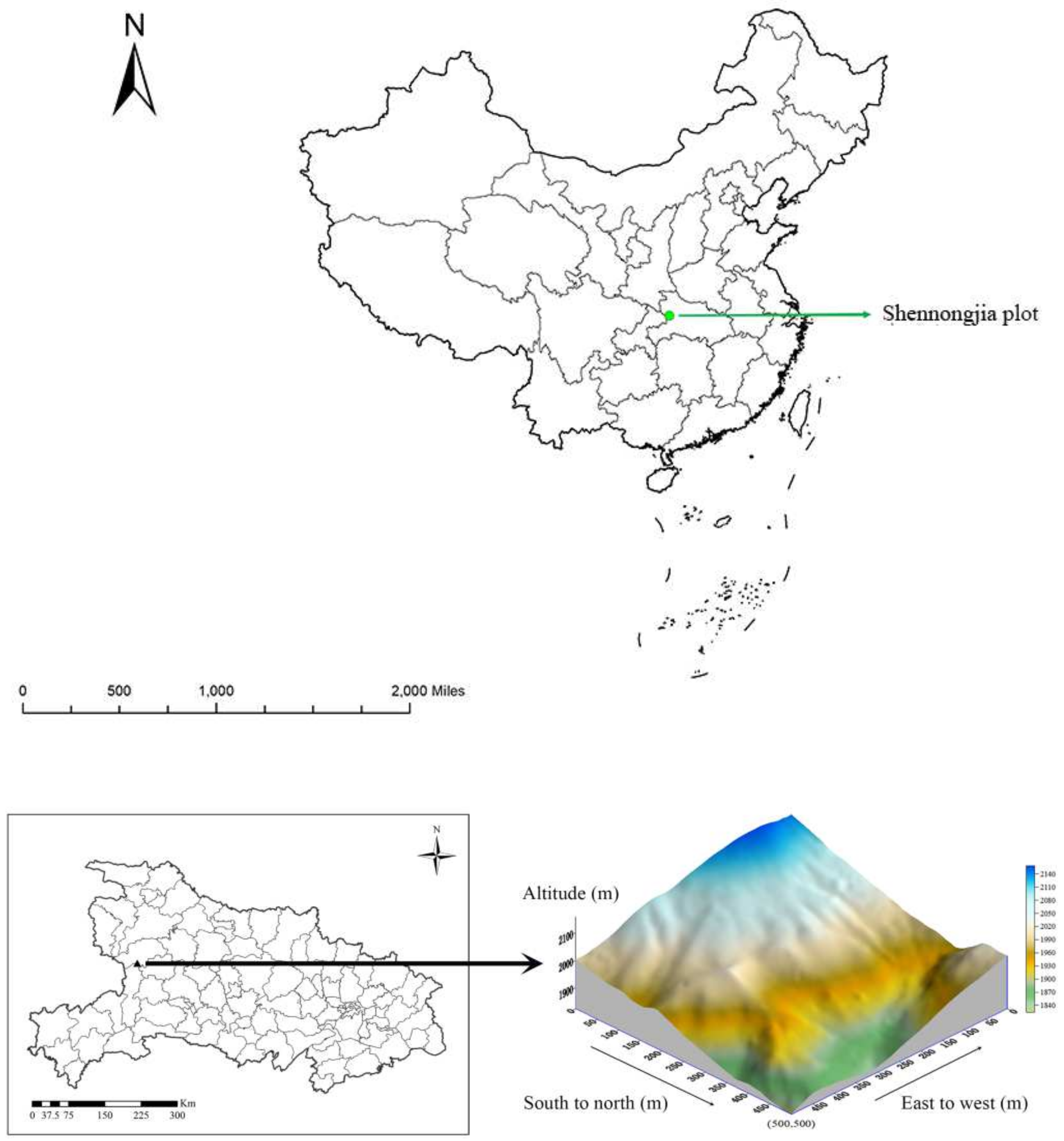
2.1. Study Site
2.2. Data Collection
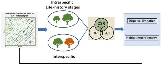
2.3. Data Analysis
2.3.1. Spatial Distribution Pattern
2.3.2. Intraspecific and Interspecific Associations
3. Results
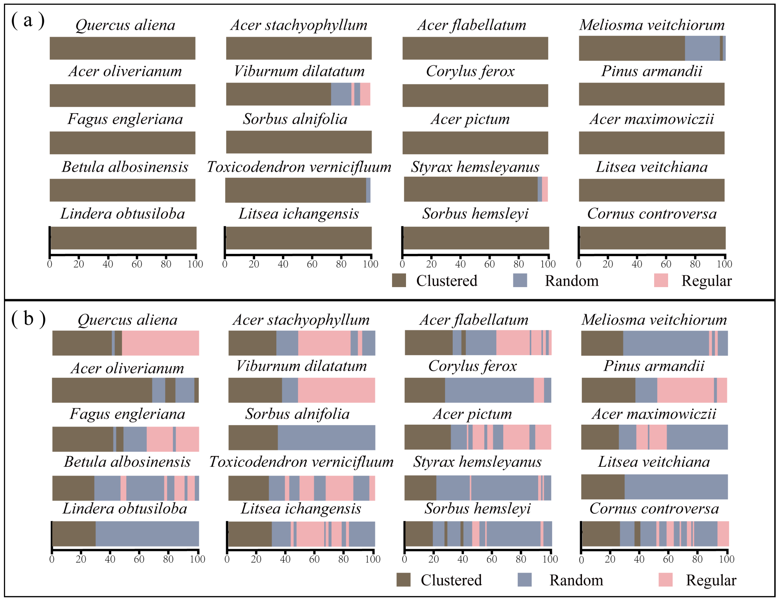
3.1. Spatial Distribution Pattern
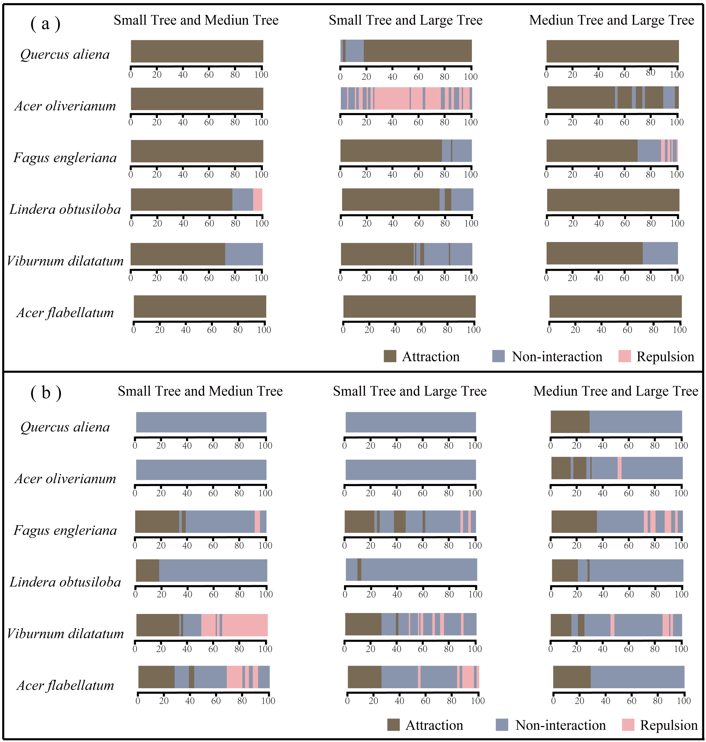
3.2. Intraspecific and Interspecific Associations
3.2.1. Intraspecific Patterns from Saplings to Adults
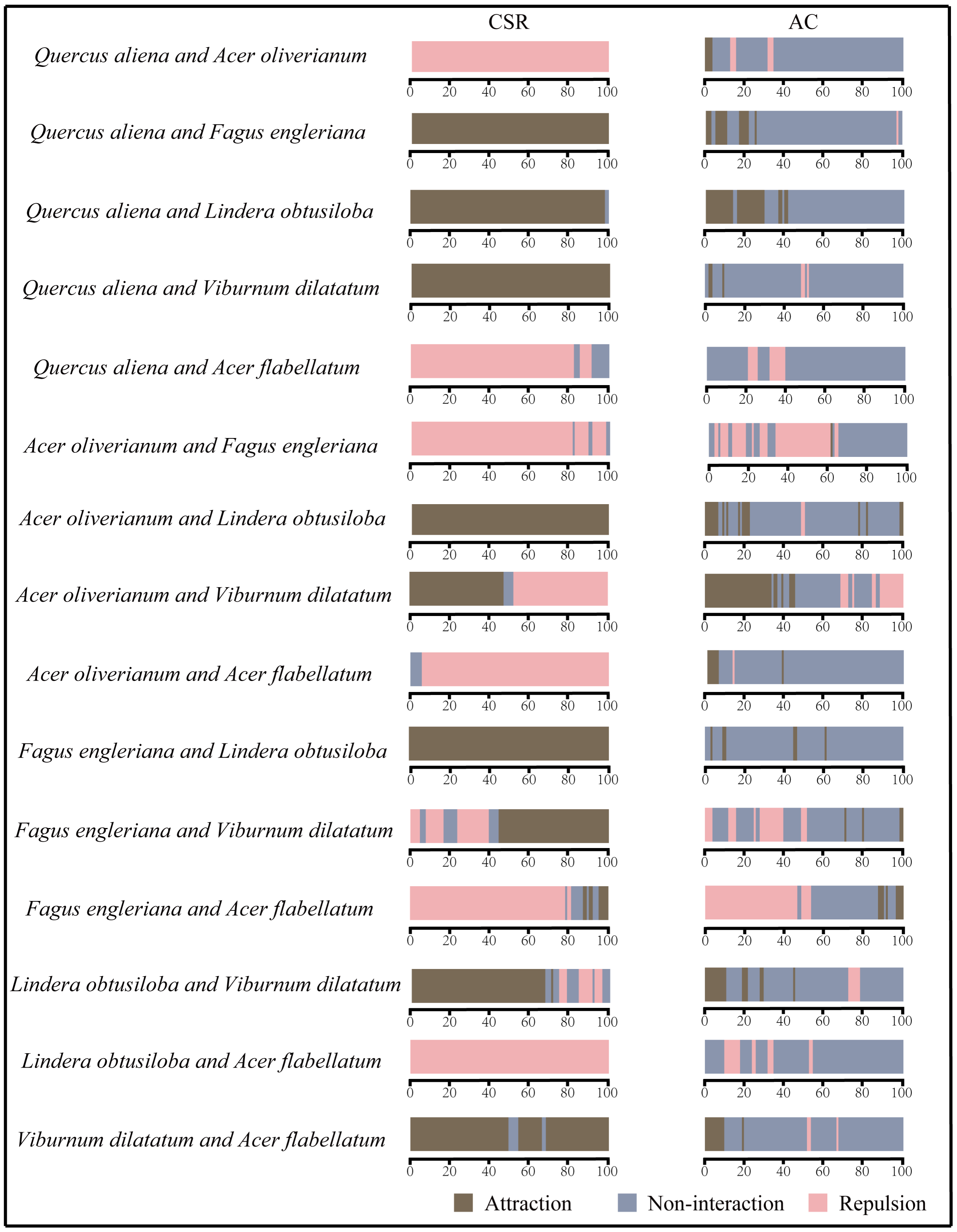
3.2.2. Interspecific Association
4. Discussion
4.1. Spatial Distributions of Dominant Species
4.2. Associations Across Species and Life-History Stages
5. Conclusions
Author Contributions
Funding
Institutional Review Board Statement
Data Availability Statement
Acknowledgments
Conflicts of Interest
References
- Wiegand, T.; Wang, X.; Anderson-Teixeira, K.J.; Bourg, N.A.; Cao, M.; Ci, X.; Davies, S.J.; Hao, Z.; Howe, R.W.; Kress, W.J.; et al. Consequences of spatial patterns for coexistence in species-rich plant communities. Nat. Ecol. Evol. 2021, 5, 965–973. [Google Scholar] [CrossRef] [PubMed]
- Lv, T.; Zhao, R.; Wang, N.-J.; Xie, L.; Feng, Y.-Y.; Li, Y.; Ding, H.; Fang, Y.-M. Spatial distributions of intra-community tree species under topographically variable conditions. J. Mt. Sci. 2023, 20, 391–402. [Google Scholar] [CrossRef]
- Janik, D.; Kral, K.; Adam, D.; Hort, L.; Samonil, P.; Unar, P.; Vrska, T.; McMahon, S. Tree spatial patterns of Fagus sylvatica expansion over 37 years. For. Ecol. Manag. 2016, 375, 134–145. [Google Scholar] [CrossRef]
- Omelko, A.; Ukhvatkina, O.; Zhmerenetsky, A.; Sibirina, L.; Petrenko, T.; Bobrovsky, M. From young to adult trees: How spatial patterns of plants with different life strategies change during age development in an old-growth Korean pine-broadleaved forest. For. Ecol. Manag. 2018, 411, 46–66. [Google Scholar] [CrossRef]
- Zhang, L.; Dong, L.; Liu, Q.; Liu, Z. Spatial Patterns and Interspecific Associations During Natural Regeneration in Three Types of Secondary Forest in the Central Part of the Greater Khingan Mountains, Heilongjiang Province, China. Forests 2020, 11, 152. [Google Scholar] [CrossRef]
- Diamond, J.M. Assembly of species communities. In Ecology and Evolution of Communities; Diamond, J.M., Cody, M.L., Eds.; Bleknap Press: Cambrige, UK, 1975; pp. 342–344. [Google Scholar]
- Weiher, E.; Keddy, P.A. Assembly rules, null models, and trait dispersion: New questions from old patterns. Oikos 1995, 74, 159–164. [Google Scholar] [CrossRef]
- Clark, D.B.; Palmer, M.W.; Clark, D.A. Edaphic factors and the landscape-scale distributions of tropical rain forest trees. Ecology 1999, 80, 2662–2675. [Google Scholar] [CrossRef]
- Zhang, Y.; Li, J.; Chang, S.; Li, X.; Lu, J. Spatial distribution pattern of Picea schrenkiana population in the Middle Tianshan Mountains and the relationship with topographic attributes. J. Arid. Land 2012, 4, 457–468. [Google Scholar] [CrossRef]
- Baldeck, C.A.; Harms, K.E.; Yavitt, J.B.; John, R.; Turner, B.L.; Valencia, R.; Navarrete, H.; Bunyavejchewin, S.; Kiratiprayoon, S.; Yaacob, A.; et al. Habitat filtering across tree life stages in tropical forest communities. Proc. R. Soc. B Biol. Sci. 2013, 280, 20130548. [Google Scholar] [CrossRef]
- Shen, G.; He, F.; Waagepetersen, R.; Sun, I.-F.; Hao, Z.; Chen, Z.-S.; Yu, M. Quantifying effects of habitat heterogeneity and other clustering processes on spatial distributions of tree species. Ecology 2013, 94, 2436–2443. [Google Scholar] [CrossRef]
- Janzen, D.H. Herbivores and the Number of Tree Species in Tropical Forests. Am. Nat. 1970, 104, 501–528. [Google Scholar] [CrossRef]
- Connell, J.H.; Tracey, J.G.; Webb, L.J. Compensatory Recruitment, Growth, and Mortality as Factors Maintaining Rain-Forest Tree Diversity. Ecol. Monogr. 1984, 54, 141–164. [Google Scholar] [CrossRef]
- Hubbell, S.P. The Unified Neutral Theory of Biodiversity and Biogeography; Princeton University Press: Princeton, NJ, USA, 2001. [Google Scholar]
- Hubbell, S.P. Tree Dispersion, Abundance, ai Diversity in a Tropical Dry Fore That tropical trees are clumped, not spac, alters conceptions of the organization and dynami. Science 1979, 203, 1299. [Google Scholar] [CrossRef]
- Wiegand, T.; Moloney, K.A. Rings, circles, and null-models for point pattern analysis in ecology. Oikos 2004, 104, 209–229. [Google Scholar] [CrossRef]
- Wiegand, T.; Moloney, K.A. Handbook of Spatial Point-Pattern Analysis in Ecology; Taylor & Francis: London, UK, 2013. [Google Scholar]
- Ben-Said, M. Spatial point-pattern analysis as a powerful tool in identifying pattern-process relationships in plant ecology: An updated review. Ecol. Process. 2021, 10, 56. [Google Scholar] [CrossRef]
- Ripley, B.D. 2nd-Order Analysis of Stationary Point Processes. J. Appl. Probab. 1976, 13, 255–266. [Google Scholar] [CrossRef]
- Gu, L.; O’Hara, K.L.; Li, W.; Gong, Z. Spatial patterns and interspecific associations among trees at different stand development stages in the natural secondary forests on the Loess Plateau, China. Ecol. Evol. 2019, 9, 6410–6421. [Google Scholar] [CrossRef]
- Erfanifard, Y.; Stereńczak, K. Intra- and interspecific interactions of Scots pine and European beech in mixed secondary forests. Acta Oecologica 2017, 78, 15–25. [Google Scholar] [CrossRef]
- Carrer, M.; Castagneri, D.; Popa, I.; Pividori, M.; Lingua, E. Tree spatial patterns and stand attributes in temperate forests: The importance of plot size, sampling design, and null model. For. Ecol. Manag. 2017, 407, 125–134. [Google Scholar] [CrossRef]
- Ge, J.; Ma, B.; Xu, W.; Zhao, C.; Xie, Z. Temporal shifts in the relative importance of climate and leaf litter traits in driving litter decomposition dynamics in a Chinese transitional mixed forest. Plant Soil 2022, 477, 679–692. [Google Scholar] [CrossRef]
- Wei, J.; Jiang, Z.; Yang, L.; Xiong, H.; Jin, J.; Luo, F.; Li, J.; Wu, H.; Xu, Y.; Qiao, X.; et al. Community composition and structure in a 25 ha mid-subtropical mountain deciduous broad-leaved forest dynamics plot in Shennongjia, Hubei, China. Biodivers. Sci. 2024, 32, 5–15. [Google Scholar] [CrossRef]
- Linares-Palomino, R.; Alvarez, S.I.P. Tree community patterns in seasonally dry tropical forests in the Cerros de Amotape Cordillera, Tumbes, Peru. For. Ecol. Manag. 2005, 209, 261–272. [Google Scholar] [CrossRef]
- Zhu, Y.; Zhao, G.F.; Zhang, L.W.; Shen, G.C.; Mi, X.C.; Ren, H.B.; Yu, M.J.; Chen, J.H.; Chen, S.W.; Fang, T.; et al. Community composition and structure of Gutianshan forest dynamics plot in a mid-subtropical evergreen broad-leaved forest, East China. J. Plant Ecol. Chin. Version 2008, 32, 262–273, (in Chinese with English abstract). [Google Scholar]
- Cressie, N.A.C. Statistics for Spatial Data, Revised ed.; John Wiley & Sons: Hoboken, NJ, USA, 2015. [Google Scholar]
- Stoyan, D. Caution with Fractal Point Patterns. Statistics 1994, 25, 267–270. [Google Scholar] [CrossRef]
- Velázquez, E.; Martínez, I.; Getzin, S.; Moloney, K.A.; Wiegand, T. An evaluation of the state of spatial point pattern analysis in ecology. Ecography 2016, 39, 1042–1055. [Google Scholar] [CrossRef]
- Jalilian, A.; Guan, Y.; Waagepetersen, R. Decomposition of Variance for Spatial Cox Processes. Scand. J. Stat. 2012, 40, 119–137. [Google Scholar] [CrossRef]
- Gabriel, E.A.; Baddeley, E.; Rubak, R. Turner: Spatial Point Patterns: Methodology and Applications with R. Mathematical Geosciences; CRC Press: Boca Raton, FL, USA, 2017. [Google Scholar]
- Baddeley, A.; Diggle, P.J.; Hardegen, A.; Lawrence, T.; Milne, R.K.; Nair, G. On tests of spatial pattern based on simulation envelopes. Ecol. Monogr. 2014, 84, 477–489. [Google Scholar] [CrossRef]
- Baddeley, A.J.; Rubak, E.; Turner, T.R. Analysing Spatial Point Patterns with R; CRC Press: Boca Raton, FL, USA, 2015. [Google Scholar]
- Perea, A.J.; Wiegand, T.; Garrido, J.L.; Rey, P.J.; Alcántara, J.M. Legacy effects of seed dispersal mechanisms shape the spatial interaction network of plant species in Mediterranean forests. J. Ecol. 2021, 109, 3670–3684. [Google Scholar] [CrossRef]
- Seidler, T.G.; Plotkin, J.B. Seed dispersal and spatial pattern in tropical trees. PLoS Biol. 2006, 4, e344. [Google Scholar] [CrossRef]
- Zhou, Q.; Shi, H.; Shu, X.; Xie, F.; Zhang, K.; Zhang, Q.; Dang, H. Spatial distribution and interspecific associations in a deciduous broad-leaved forest in north-central China. J. Veg. Sci. 2019, 30, 1153–1163. [Google Scholar] [CrossRef]
- Lin, G.; Stralberg, D.; Gong, G.; Huang, Z.; Ye, W.; Wu, L. Separating the effects of environment and space on tree species distribution: From population to community. PLoS ONE 2013, 8, e56171. [Google Scholar] [CrossRef] [PubMed]
- Getzin, S.; Wiegand, T.; Wiegand, K.; He, F. Heterogeneity influences spatial patterns and demographics in forest stands. J. Ecol. 2008, 96, 807–820. [Google Scholar] [CrossRef]
- Beyns, R.; Bauman, D.; Drouet, T. Fine-scale tree spatial patterns are shaped by dispersal limitation which correlates with functional traits in a natural temperate forest. J. Veg. Sci. 2021, 32, e13070. [Google Scholar] [CrossRef]
- Hardy, O.J.; Sonké, B. Spatial pattern analysis of tree species distribution in a tropical rain forest of Cameroon: Assessing the role of limited dispersal and niche differentiation. For. Ecol. Manag. 2004, 197, 191–202. [Google Scholar] [CrossRef]
- Dohn, J.; Augustine, D.J.; Hanan, N.P.; Ratnam, J.; Sankaran, M. Spatial vegetation patterns and neighborhood competition among woody plants in an East African savanna. Ecology 2017, 98, 478–488. [Google Scholar] [CrossRef]
- Peters, H.A. Neighbour-regulated mortality: The influence of positive and negative density dependence on tree populations in species-rich tropical forests. Ecol. Lett. 2003, 6, 757–765. [Google Scholar] [CrossRef]


| Species Name | Family Name | Abundance | Basal Area (m2/ha) | Maximum DBH (cm) | Importance Value | Life Form |
|---|---|---|---|---|---|---|
| Quercus aliena var. acutiserrata | Fagaceae | 2141 | 136.12 | 105.92 | 0.0749 | D |
| Acer oliverianum | Sapindaceae | 7556 | 109.66 | 51.80 | 0.0742 | D |
| Fagus engleriana | Fagaceae | 2345 | 95.90 | 83.50 | 0.0663 | D |
| Betula albosinensis | Betulaceae | 1670 | 50.56 | 102.23 | 0.0571 | D |
| Lindera obtusiloba | Lauraceae | 2552 | 50.50 | 59.82 | 0.0455 | D |
| Acer stachyophyllum subsp. betulifolium | Sapindaceae | 3284 | 31.80 | 21.22 | 0.0310 | D |
| Viburnum dilatatum | Adoxaceae | 3089 | 22.93 | 14.45 | 0.0277 | D |
| Sorbus alnifolia | Rosaceae | 1951 | 19.01 | 42.36 | 0.0248 | D |
| Toxicodendron vernicifluum | Anacardiaceae | 924 | 17.27 | 53.60 | 0.0247 | D |
| Litsea ichangensis | Lauraceae | 2075 | 15.08 | 48.11 | 0.0223 | D |
| Acer flabellatum | Sapindaceae | 1700 | 13.45 | 52.56 | 0.0211 | D |
| Corylus ferox var. thibetica | Betulaceae | 1376 | 12.97 | 49.31 | 0.0190 | D |
| Acer pictum subsp. mono | Sapindaceae | 1679 | 12.93 | 47.80 | 0.0190 | D |
| Styrax hemsleyanus | Styracaceae | 1208 | 12.22 | 47.10 | 0.0183 | D |
| Sorbus hemsleyi | Rosaceae | 805 | 11.89 | 92.99 | 0.0176 | D |
| Meliosma veitchiorum | Sabiaceae | 801 | 11.50 | 97.50 | 0.0170 | D |
| Pinus armandii | Pinaceae | 972 | 10.66 | 78.47 | 0.0166 | E |
| Acer maximowiczii | Sapindaceae | 1234 | 10.48 | 32.12 | 0.0164 | D |
| Litsea veitchiana | Lauraceae | 1443 | 10.49 | 20.11 | 0.0163 | D |
| Cornus controversa | Cornaceae | 695 | 9.66 | 49.40 | 0.0158 | D |
| Species Name | Layer | Abundance | Individuals of Small Trees | Individuals of Medium Trees | Individuals of Large Trees |
|---|---|---|---|---|---|
| Quercus aliena var. acutiserrata | Canopy | 2141 | 222 | 718 | 1201 |
| Acer oliverianum | Understory | 7556 | 4613 | 1673 | 1270 |
| Fagus engleriana | Canopy | 2345 | 824 | 899 | 622 |
| Lindera obtusiloba | Understory | 2552 | 368 | 617 | 1567 |
| Viburnum dilatatum | Shrub | 3089 | 1874 | 384 | 231 |
| Acer flabellatum | Understory | 1700 | 1135 | 337 | 228 |
Disclaimer/Publisher’s Note: The statements, opinions and data contained in all publications are solely those of the individual author(s) and contributor(s) and not of MDPI and/or the editor(s). MDPI and/or the editor(s) disclaim responsibility for any injury to people or property resulting from any ideas, methods, instructions or products referred to in the content. |
© 2025 by the authors. Licensee MDPI, Basel, Switzerland. This article is an open access article distributed under the terms and conditions of the Creative Commons Attribution (CC BY) license (https://creativecommons.org/licenses/by/4.0/).
Share and Cite
Wei, J.; Yang, L.; Jiang, Z.; Yao, H.; Yu, H.; Luo, F.; Qiao, X.; Xu, Y.; Jiang, M. Spatial Distribution and Intraspecific and Interspecific Associations of Dominant Tree Species in a Deciduous Broad-Leaved Forest in Shennongjia, China. Diversity 2025, 17, 335. https://doi.org/10.3390/d17050335
Wei J, Yang L, Jiang Z, Yao H, Yu H, Luo F, Qiao X, Xu Y, Jiang M. Spatial Distribution and Intraspecific and Interspecific Associations of Dominant Tree Species in a Deciduous Broad-Leaved Forest in Shennongjia, China. Diversity. 2025; 17(5):335. https://doi.org/10.3390/d17050335
Chicago/Turabian StyleWei, Jiaxin, Linsen Yang, Zhiguo Jiang, Hui Yao, Huiliang Yu, Fanglin Luo, Xiujuan Qiao, Yaozhan Xu, and Mingxi Jiang. 2025. "Spatial Distribution and Intraspecific and Interspecific Associations of Dominant Tree Species in a Deciduous Broad-Leaved Forest in Shennongjia, China" Diversity 17, no. 5: 335. https://doi.org/10.3390/d17050335
APA StyleWei, J., Yang, L., Jiang, Z., Yao, H., Yu, H., Luo, F., Qiao, X., Xu, Y., & Jiang, M. (2025). Spatial Distribution and Intraspecific and Interspecific Associations of Dominant Tree Species in a Deciduous Broad-Leaved Forest in Shennongjia, China. Diversity, 17(5), 335. https://doi.org/10.3390/d17050335