Environmental DNA for Assessing Population and Spatial Distribution of Spinibarbus caldwelli in the Liuxi River

Abstract

The wild resources of Spinibarbus caldwelli, once an important economic fish in southern China, have been drastically reduced in recent years due to environmental changes and human activities. The Liuxi River S. caldwelli National Aquatic Germplasm Reserve was established in Conghua District, Guangzhou city, and the release of S. caldwelli was carried out. However, traditional fishery resource survey methods yield less accurate results when the abundance of the surveyed species is low or when they are difficult to catch. As a non-destructive and non-invasive approach, environmental DNA (eDNA) is widely employed in aquatic species monitoring, though its detection efficiency may be affected by environmental conditions. Therefore, this study explored the eDNA monitoring methods of S. caldwelli in Liuxi River from the following four aspects: (1) the relationship between eDNA release and biomass/abundance; (2) the concentration and diffusion range of eDNA over time in a lentic ecosystem; (3) the diffusion range of eDNA in a lotic ecosystem; and (4) the effects of eDNA application in field monitoring. Our results showed a correlation between eDNA concentration and abundance/biomass of S. caldwelli. eDNA of S. caldwelli can diffuse up to 18 m in lentic ecosystems within 2 h and decreases with distance. eDNA of S. caldwelli released by 10 individuals in Liuxi River could be detected 900 m downstream. Field studies in Liuxi River showed that the eDNA method has high sensitivity in detecting the presence or absence of species and is highly consistent with the results of traditional methods. This study explored the application of environmental DNA technology in species monitoring in Liuxi River. Our aim was to evaluate the applicability and potential of eDNA in ecological monitoring of stream fishes.

1. Introduction

The continuing decline of biodiversity is one of the major challenges of the twenty-first century [1]. According to the Living Planet Index of the World Wide Fund for Nature (WWF), global wildlife populations have declined by 60 per cent since 1970, and the rate of decline for freshwater organisms has reached 83 per cent [2]. The urgency of biodiversity monitoring has never been greater [3], yet the status of biodiversity in many taxa and regions remains unclear or even unstudied [4]. Biodiversity is the basis for human survival and development [5], so comprehensive and accurate ecological monitoring is essential under the premise of protecting the existing ecological environment [6]. Conservation of biodiversity begins with biological surveys and monitoring to obtain data on species distribution and population size. Traditional monitoring methods rely mainly on morphological identification and counting of individuals in the field, which require experienced specialists and present a number of survey challenges in aquatic ecosystems where some fish are small, few, or difficult to catch [7]. Traditional survey methods such as trawling, seining, and electrofishing are not only time-consuming and costly, but may also cause harm to the fish [8]. Environmental DNA technology, as an emerging tool, provides a simple, non-invasive solution for biodiversity monitoring and can be widely used for ecological monitoring.

In general, environmental DNA refers to the genetic material released into the surrounding environment by all organisms, including skin, mucus, and excreta [9,10,11]. Environmental DNA can be divided into individual (e.g., plankton) and non-individual (tissue or mucus) DNA and can be further subdivided into intracellular and extracellular eDNA, with the latter usually found in freshly shed cells. Once released from its source, DNA spreads rapidly, meaning that the presence of a target species can theoretically be detected anywhere in the water column, not just near the source of its release. However, DNA in the environment may gradually break down and eventually disappear due to UV exposure and microbial degradation. Therefore, the eDNA signal of a target species can provide evidence of its current or recent presence without relying on direct observation or actual capture [10].

Ficetola et al. (2008) successfully detected invasive bullfrogs in the United States through eDNA in ponds, marking the first successful application of eDNA technology in an aquatic environment [12]. Since then, research has continued to focus on invasive species detection, such as Dejean et al., who also used eDNA to study bullfrogs, confirming its advantages in invasive species monitoring [13]. Early application of eDNA methods to detect potential fecal contamination in aquatic systems was done by Martellini et al. [14]. In recent years, environmental DNA technology has been rapidly developing in a number of fields, including food, microbiology, biomonitoring, ecology, and conservation biology [15]. The results of eDNA detection in water samples can accurately reflect the current status of the ecosystem [16,17]. eDNA technology has been widely used in aquatic biomonitoring, including the study of amphibians, reptiles, fish, and aquatic invertebrates, and these relevant results indicate that eDNA has significant effects in species detection and stock assessment [6,7,18]. Therefore, eDNA concentration can be a fast, efficient, and economical indicator of species abundance or biomass in fisheries stock assessment [11]. The relationship between eDNA concentration and species abundance has been validated in various controlled and field studies, where researchers observed a positive correlation between the amount of eDNA detected and the biomass of target species [18,19].

However, there are discrepancies in the results of the studies [17,18,20,21]. Its application in assessing fish abundance, biomass, and distribution in both lentic and lotic ecosystems requires further validation. Transport of eDNA is also a key factor in assessing the amount of species resources. Although several researchers have explored eDNA transport in moving water environments [22,23,24,25,26,27,28], they have different views due to differences in experimental subjects, sites, and sampling methods.

Spinibarbus caldwelli (Nichols, 1925) is an endemic species to China. It has an anterior cylindrical body, a posterior laterally compressed body, an equal-sized eye, and a rounded muzzle. It belongs to the order Cypriniformes, family Carpidae, which is mainly found in the Yuanjiang River, Pearl River, Jiulongjiang River, Minjiang River, Yangtze River, and Hainan Island [29]. Since populations of S. caldwelli have declined significantly and their genetic diversity has been substantially reduced, the species is now listed as endangered by the IUCN [30]. While eDNA technology demonstrates high sensitivity and cost-effectiveness as an emerging fisheries monitoring tool—particularly for detecting low-density fish populations [15,21,31]—its application in population abundance assessments requires further validation. Due to factors such as hydraulic engineering structures, water pollution, and overfishing, the wild populations of S. caldwelli have experienced severe declines [32]. To advance the application of eDNA technology in aquatic species monitoring and conservation, this study conducted the following four experiments using S. caldwelli as the focal species:

• Tank experiment: exploring the relationship between environmental DNA and abundance/biomass.
• Pool cage fish experiment: analyzing the diffusion distance of eDNA in a lentic ecosystem.
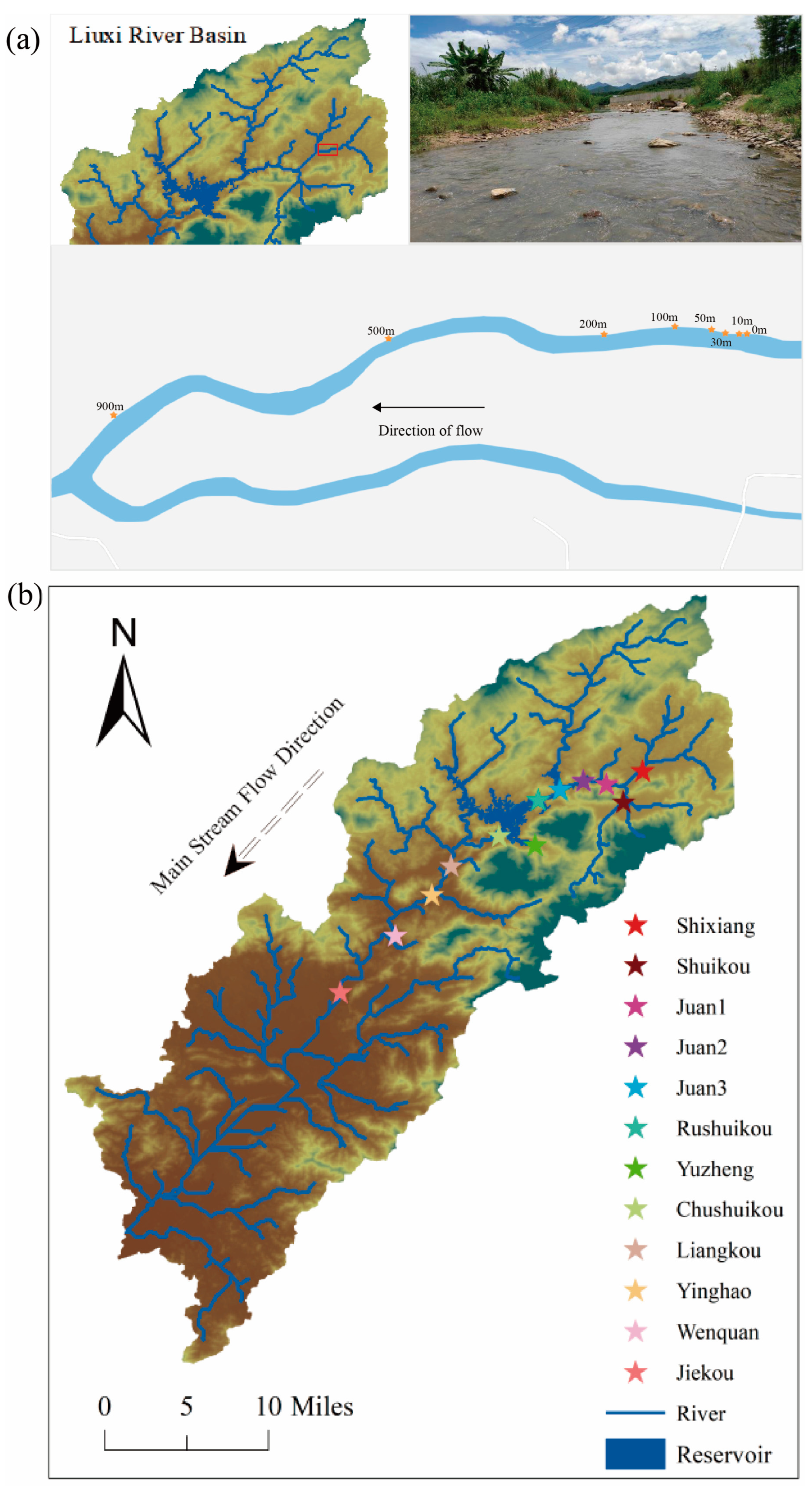
• Field cage fish experiment: studying the diffusion distance of eDNA in a lotic ecosystem.
• Experiment on monitoring the resources of S. caldwelli in the Liuxi River: investigating the distribution and population size of S. caldwelli by using environmental DNA technology and comparing the data with those obtained by traditional methods.

By integrating these experiments, we aim to establish a scientific basis for the application of eDNA in freshwater fish conservation, particularly for the management of S. caldwelli populations.

2. Materials and Methods

2.1. Experimental Strategy

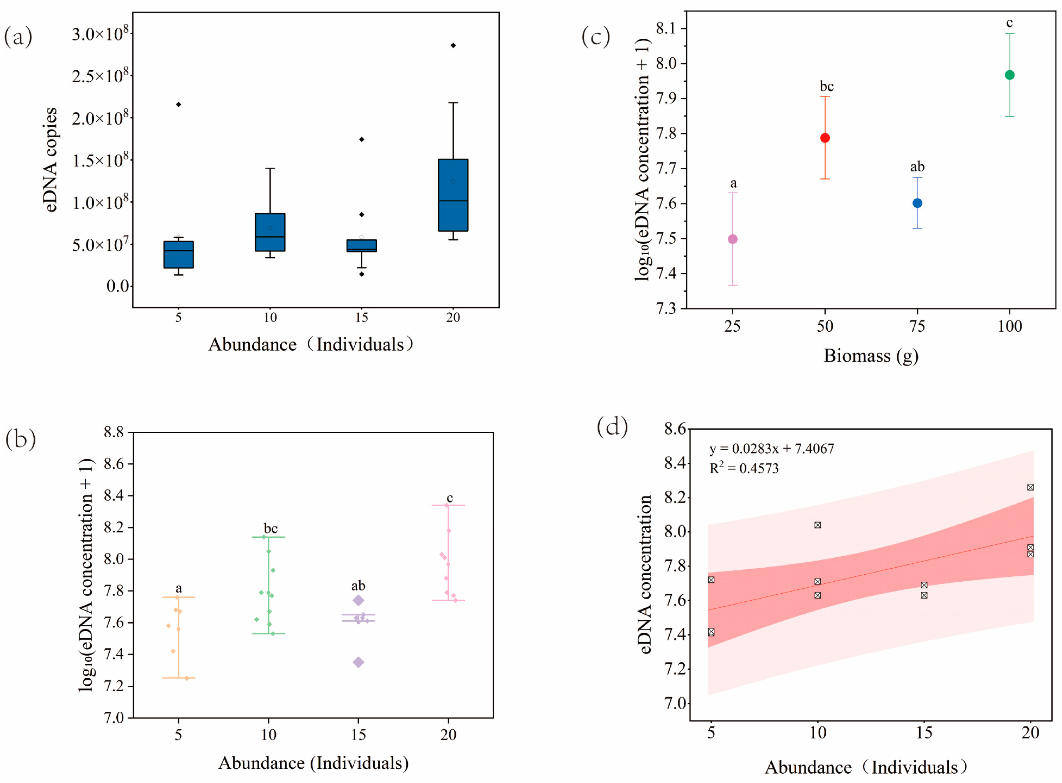
2.1.1. Tank Experiment: Relationship Between eDNA Concentration and Abundance/Biomass

In order to observe the relationship between environmental DNA concentration and S. caldwelli abundance/biomass, we prepared juvenile S. caldwelli (5–7 cm, 5.00 ± 1.26 g), 15 culture tanks (25 L), and hand nets for indoor observation experiments. The specific steps were as follows: All culture tanks were filled with 20 L of tap water. After full aeration for two days, we placed the juvenile fish into each plastic bucket according to the quantity gradient (0, 5, 10, 15, 20 fish) and set up three replicates for each gradient. After putting in the air tube of the oxygen pump, the lid of the tank was closed (leaving a gap) to prevent the juvenile fish from jumping out. No feeding was done during the experiment. At the end of the experiment, we randomly removed 42 juvenile fish, anaesthetized them using an anesthetic, and measured their body length and body mass. The flow of the experiment is shown in Figure 1a.

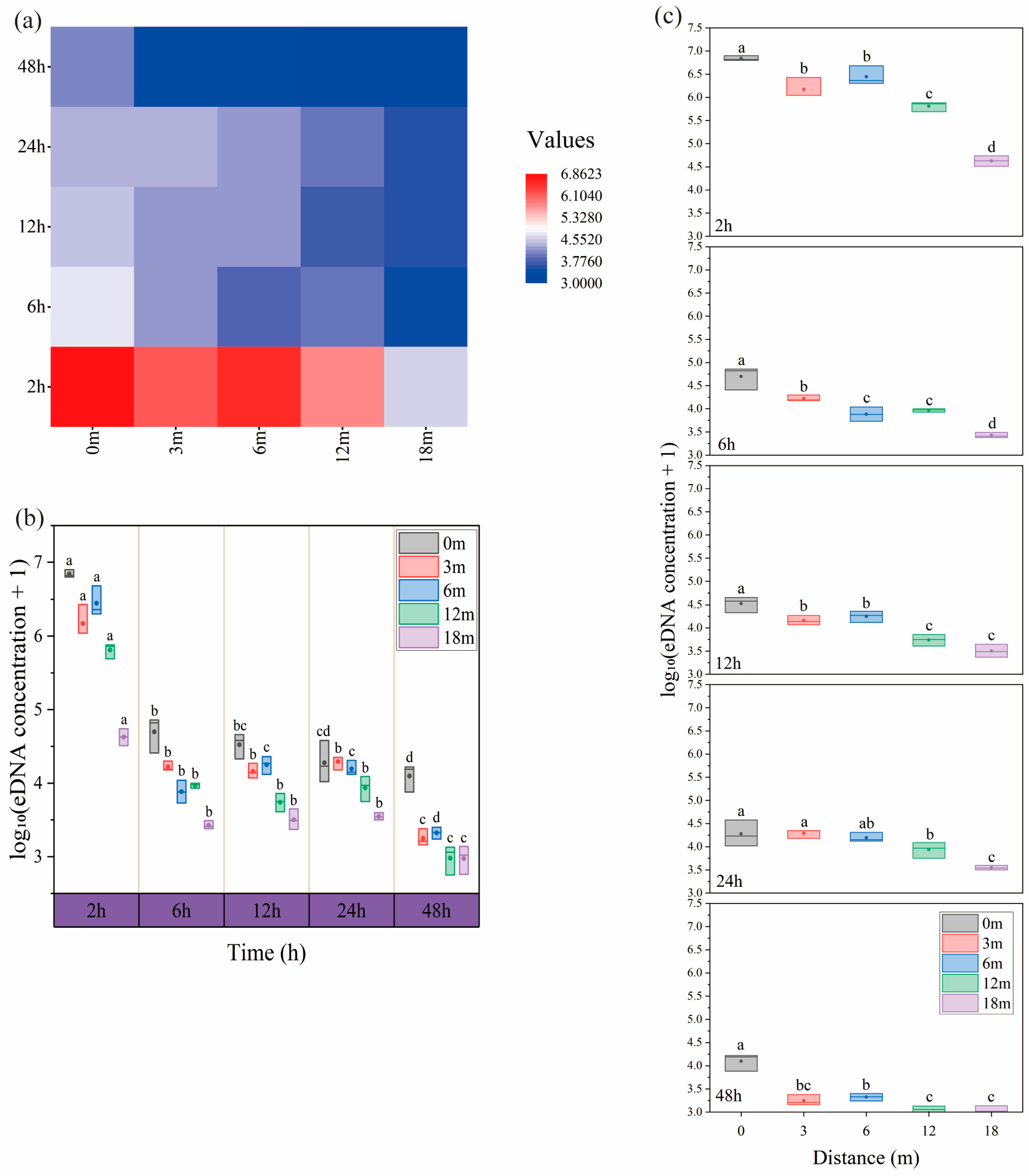
2.1.2. Lentic Ecosystem: Diffusion of eDNA

In this study, we selected a concrete culture pond with dimensions of about 19 m long, 4 m wide, and 1.8 m high, and the water depth was maintained at 112 cm during the experimental period. Ten S. caldwelli subadults were selected (body mass of 279.99 ± 74.6 g) and placed into a round cage with a diameter of 1 m and a height of 1 m, and the cage was suspended at one end of the pond. In order to confirm the diffusion range of eDNA, we set up five sampling points, 0 m, 3 m, 6 m, 12 m, and 18 m, according to the position of the cage (Figure 1b). Meanwhile, to monitor the release time of eDNA, water samples were collected at 2 h, 6 h, 12 h, 24 h, and 48 h after the cage was placed. Although the oxygen pump in the pool was on during the experiment, we reduced the airflow rate to 36.72 mL/h to try to minimize the disturbance to the still water state caused by airflow. The schematic diagram of the experiment is shown in Figure 1b.

2.1.3. Lotic Ecosystem: Diffusion of eDNA

The study site was selected as a small tributary of the Liuxi River near Lvtian Town, Conghua District, Guangzhou City, Guangdong Province, China (Figure 2a). The selected section of the river had a cobble bed with a sandy substrate and clear water with an average depth of about 40 cm (Figure 2a). From May to July each year, the S. caldwelli would swim upstream from the Liuxi River Reservoir to this location to gather and spawn. At the beginning of the experiment, the spawning period of the S. caldwelli was over, and the presence of the S. caldwelli was not observed during the collection of blank samples. We set up eight sampling points in this experiment, marked as 0 m, 10 m, 30 m, 50 m, 100 m, 200 m, 500 m, and 900 m, according to the direction of flow of the river (Figure 2a). On 6 August 2020, we walked along the river to observe the presence of target fish, and 1 L of water per sampling point was collected as a negative control. On 7 August 2020, 10 subadults (mean body mass 91.3 g ± 28.6 g) were placed in a circular cage 1 m in diameter and 1 m in height and suspended from the 0 m sampling point. The cage was left to stand for 24 h. On 8 August 2020, sampling was carried out sequentially along the river, starting from the 900 m sampling point. The cross-sectional sampling method was used, with 1 L of water sampled on either side of the riverbank and in the middle of the river at each sampling point, for a total of 24 samples.

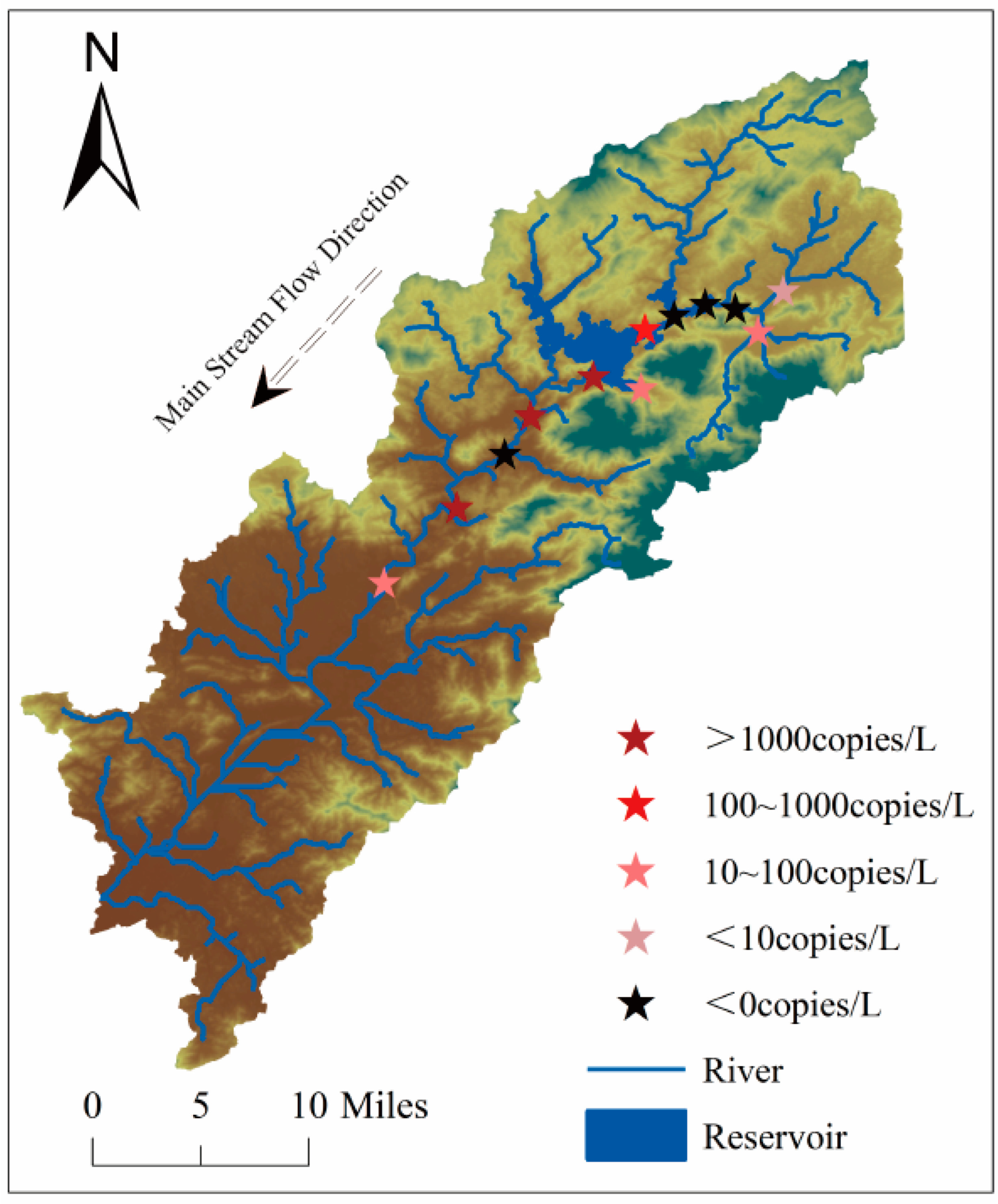
2.1.4. Liuxi River Survey: Monitoring Effectiveness of eDNA Methodology

In this study, the eDNA method was applied to sample the Liuxi River in Conghua District, Guangzhou City. The obtained data were compared with those collected through traditional methods to evaluate the sensitivity of eDNA technology. A total of 12 sampling points were established from upstream to downstream: Shixiang, Shuikou, Juan 1, Juan 2, Juan 3, Rushuikou, Yuzheng, Chushuikou, Liangkou, Yinghao, Wenquan, and Jiekou (Figure 2b).

We already had some of the data from the traditional methods before conducting the eDNA experiments. In 2020, we were on schedule for traditional methods while we conducted eDNA studies. From December 2017 to October 2020, we conducted a total of nine sampling events using traditional methods at four sampling sites in the Liuxi River (Shuikou, Rushuikou, Yinghao, Jiekou) (Table S8). Traditional methods of sampling mainly used gillnets, ground cages, and plunge nets, adapted to the habitat, weather conditions, and local management requirements. Sampling was carried out one to three times per year, and if S. caldwelli was caught on one of these occasions, it was considered a positive result; if no S. caldwelli was caught throughout the year, it was recorded as a negative result (Table S9).

Local management authorities conduct annual stocking and releasing of S. caldwelli to restore the wild population resources. The Liuxi River Reservoir serves as a major fattening site for the S. caldwelli and a core conservation area for its germplasm resources, so the Yuzheng sampling site in the reservoir is a fixed annual stock enhancement and release site, while the other sampling sites are experimental area release sites, which are changed every year (Table S9).

2.2. Primer/Probe Design

In this experiment, we designed specific primers based on the mitochondrial COI gene for the S. caldwelli and its close relatives in the Liuxi River, Conghua District, Guangzhou City. The COI sequences of S. caldwelli were obtained from the NCBI database (sequence numbers MF123265.1 and MF123264.1). Additionally, we obtained de novo sequences from local individuals by extracting DNA from fin tissue and amplifying the fragment by PCR in a 25 µL reaction mixture consisting of 12.5 µL of 2× Taq PCR Master Mix (BGI, Shanghai, China), 1 µL of each primer (forward and reverse), 1 µL of template DNA, and 9 µL of ddH₂O. Amplicons were sent to Tsingke Bio Co., Ltd., Beijing, China, for sequencing.

COI TY—Forward primer: TACTAATCACAAAGACATTGGCAC

COI TY—Reverse primer: TAAACTTCTGGGTGGCCAAAGAATCA

The COI sequences of all other fish species were obtained from the NCBI database. In the Liuxi River, closely related species include the Puntius semifasciolatus (Günther, 1868; KJ994663.1), Carassius auratus (Linnaeus, 1758; HM392047.1), Cyprinus carpio (Linnaeus, 1758; JX983283.1), Acrossocheilus parallens (Nichols, 1931; KJ994628.1), Acrossocheilus spinifers (Wu & Zhang, 2006; NC_034918.1), Cirrhinus mrigala (Hamilton, 1822; KU559566.1), Cirrhinus molitorella (Valenciennes, 1844; GU086576.1), Onychostoma gerlachi (Peters, 1881; KJ994644.1), and Osteochilus salsburyi (Nichols & Pope, 1927; GU086577.1).

We imported the COI sequences of S. caldwelli and its close relatives into MEGA 7 software for comparison and designed specific primers and probes using Primer Express 3.0 (Tables S1–S3), and the final amplified fragment length was 138 bp. Primer matching through the NCBI database showed that the primer was specific only for S. caldwelli in Liuxi River fish. However, due to the high degree of similarity in mitochondrial gene sequences in Cyprinidae, PCR validation showed that non-specific bands appear in other fish samples at higher concentrations (1 × 10⁻³ ng/μL); however, at low concentration conditions (1 × 10⁻⁵ ng/μL), only S. caldwelli DNA was amplified (Figure S1). Pre-experiments showed very low eDNA concentrations (1 × 10⁻⁶ to 1 × 10⁻⁹ ng/μL) in the water samples collected in the Liuxi River. In the qPCR experiments, probes with the same specificity were also added to ensure the specificity and accuracy of the qPCR assay.

2.3. Plasmid Standard Preparation

The reared S. caldwelli were fished from the laboratory breeding pond, and a small piece of caudal fin was clipped and preserved in 95% ethanol. DNA extraction was carried out using the Shanghai Sangon Ezup Column Animal Genomic DNA Extraction Kit.

The extracted DNA of S. caldwelli was amplified by PCR using COI primers (COI TY forward/COI TY reverse, same as 2.2). The PCR products were then sent to Tsingke Biotechnology Co., Ltd. for Sanger sequencing. The sequencing results were compared with the NCBI database, and the match was over 99%. The PCR product was ligated into pClone007 Blunt plasmid and transferred into E. coli receptor cells E. coli DH5α. After night culture, single clones were picked up, and the positive strains were screened by PCR, and then sent to Tsingke for sequencing. The results showed that the COI fragment of S. caldwelli was successfully ligated to the pClone007 Blunt plasmid. The bacterial solution was stored in −80 °C refrigerator by adding an equal volume of glycerol. When used, the strains were removed from the −80 °C refrigerator, amplified overnight, and the plasmid DNA was extracted using the Shanghai Sangong Column Plasmid DNA Small Volume Extraction Kit (B110091-0050, BGI, Shanghai, China).

2.4. eDNA Sample Collection/Filtration

Sampling bottles and filtration apparatus were decontaminated by immersion in a 0.1% bleach solution for 30 min, followed by thorough rinsing with tap water and ultrapure water before drying. The samples were then filtered using a vacuum diaphragm pump (GM-1.0A, Jinteng, Tianjin, China), a triplex filtration device (JIFA0211, Jinteng, Tianjin, China), and a 0.7 μm glass fiber filter membrane (1825-047, Whatman, Medstone, UK) [33,34,35,36,37,38]. During DNA extraction, all extraction devices and forceps were similarly treated with bleach solution, rinsed, and moistened with ultrapure water to prevent cross-contamination.

We filtered 1 L of store-bought purified water as a device blank prior to pumping the sample. After filtration was completed, the filter membrane was folded twice to form a fan shape, wrapped in tin foil, placed in a labelled Ziploc bag, and stored frozen at −20 °C for subsequent DNA extraction.

2.4.1. Tank Experiment

Juvenile S. caldwelli were tanked and left to stand for one day. Three 1 L water samples were collected from each tank separately on the second day. All samples were collected from each tank and immediately filtered. A total of six hours was spent from the start of collection to the end of filtration.

2.4.2. Lentic Ecosystem

Cages containing 10 S. caldwelli were hung at one end of the concrete pool. Prior to the experiment, we verified the absence of eDNA in the pond using qPCR. Water samples (1 L each) were collected from the two ends and the middle of the pond to ensure spatial representation. At each sampling point, three 1 L water samples were collected at different time intervals of 2, 6, 12, 24, and 48 h after placement. Gloves were changed at the end of each sampling session to avoid sample contamination. Since the cement pond is only 30 m from the laboratory, a cold box was not required for sample transport. Each round of sampling lasts approximately 40 min, and filtration was carried out immediately after sampling, with each filtration round lasting approximately 1.5 h.

2.4.3. Lotic Ecosystem

Studies have shown that the addition of BAC solution can effectively prolong the stability of environmental DNA [39]. To prevent degradation of environmental DNA, 1 mL of 10% benzalkonium chloride (BAC, Aladdin Biochemical Technology Co., Ltd., Shanghai, China) solution was added to 1 L of water sample immediately after collection. To avoid contamination, the bottles were dried of water droplets after each sampling, and then the surface of the sampling bottles was wiped with bleach solution, after which the disposable gloves were replaced. Samples were placed in a cool box to maintain a low temperature and dark environment and were quickly transported back to the laboratory for filtration. Due to the high level of impurities in the river water, 500 mL of water samples were filtered through a membrane. Filter membranes for the same water sample were wrapped in the same piece of tin foil.

2.4.4. Liuxi River Survey

Water samples were collected using cross-sectional sampling, with 1 L samples obtained at three positions across the channel: left bank, right bank, and mid-channel. A water sampler was used to collect water samples from the middle and lower layers of the river as much as possible. A 10% benzalkonium chloride (BAC) solution was added to the collected water samples to retard DNA degradation. After collection, the bottles were dried of water droplets with a paper towel and then wiped with a paper towel dipped in 0.1% bleach solution to avoid cross-contamination between different sampling points. The samples were kept in a cool box to maintain a low temperature and transported back to the laboratory as soon as possible for filtration. Each filter membrane was used to process 500 mL of water. For 1 L of water samples, two membranes were used and wrapped together in the same piece of tin foil.

2.5. eDNA Extraction

DNA was extracted from the filter membranes using the Blood and Tissue Kit (Qiagen, Hilden, Germany) following the manufacturer’s protocol with the following modifications:

For eDNA samples from natural rivers and streams, which required the simultaneous extraction of two filter membranes (resulting in a larger volume), the volumes of AL buffer and PK were increased to 600 μL and 60 μL, respectively, to ensure complete immersion and efficient extraction of environmental DNA. To improve the recovery of eDNA on the filter membrane, after centrifugation with AL buffer and Proteinase K (PK), 220 μL of TE buffer (BGI, Shanghai, China) was added to each sample, followed by another centrifugation step. Finally, DNA was eluted using 110 μL of AE buffer. The eluted DNA was stored at −20 °C for subsequent qPCR analysis.

To avoid contamination, DNA extraction was performed in a laboratory environment free of PCR products. Also, the same forceps were limited to one sample of membrane. Additionally, before placing the saliva collection tubes in the water bath, the lower half of the tube was slightly loosened to create a small gap, preventing excessive air pressure buildup during incubation.

2.6. Sensitivity Testing

Plotting standard curves using known concentrations of eDNA to calculate DNA copy number can be used to quantitatively analyze the concentration of eDNA. The qPCR using TaqMan probes is considered to be the most efficient method currently available for detecting eDNA in a single species [40]. Probe qPCR provides higher specific detection and quantification capabilities and is often recommended as an a priori method for species detection [41,42]. The COI fragments were amplified using a Bio-Rad real-time fluorescent quantitative PCR system (CFX96, Bio-Rad Laboratories, Inc., Hercules, USA) or a Roche fluorescent quantitative PCR instrument (LightCycler^®96, F. Hoffmann-La Roche Ltd., Basel, Switzerland). Primers and probes that had been designed were synthesized and used with the following sequences:

(1) CB COI-F: ATCAATCCTAGGGGGCAATCAATT

(2) CB COI-R: TAAAACAGGTAGTGATAGAAGGAGTAGTA

(3) CB COI-Probe: FAM-GGCGGGTTACAAGTACAGAT-MGB

Each qPCR reaction volume was 20 μL, including: DNA template, forward and reverse primers at a final concentration of 900 nM, probes at a final concentration of 125 nM, qPCR master mix (TaqMan Environmental Master Mix 2.0, Life Technologies, Scotland, UK), UDG enzyme (LM11042, Lianmai, Beijing, China), and ultrapure water (Table S4 for specific systems). The qPCR thermocycling reaction procedure is shown in Table S5. Each qPCR consisted of five gradient dilutions of the standard curve (standard curve ready to use), negative control (ddH₂O), and three replicates per sample. Standard curves were constructed from gradient-diluted plasmids, which were the same plasmid constructions described in Section 2.3 (provided by Tsingke Bio Co., Ltd., Beijing, China) Samples with Cq values above 40 are suspicious and should not normally be reported, but using an arbitrary Cq cutoff is again not ideal [43]. The detection threshold was determined based on the standard curve. Samples were considered negative if their Cq values exceeded the highest dilution that successfully amplified or were higher than those of the ultrapure water control. The limit of detection (LOD) was established through primer efficiency calculations to ensure a more accurate threshold [44]. If a sample’s three replicates yielded inconsistent results near the detection threshold, additional experiments were conducted to verify the outcome.

2.7. Statistical Processing and Analysis of Data

2.7.1. Tank Experiment

Three parallel tanks were set up for each abundance gradient, and three water samples were collected from each tank. Three qPCR replicates were performed for each water sample, and the average copy number of the three qPCR replicates was taken as the eDNA copy number for that sample. The copy number/filter volume was used as the eDNA concentration of the sample. A box-and-line plot was used to demonstrate eDNA concentration and to exclude outlier copy values. After excluding the outlier values, the data were analyzed as follows:

To improve homogeneity of variance, copy numbers were Log₁₀(x + 1)-transformed. Tests for homogeneity of variance were performed by Levene’s test, significant differences in eDNA concentration across abundance/biomass were analyzed by one-way ANOVA, and further multiple comparisons were performed using Duncan’s test. The biomass of the juveniles was calculated by multiplying the abundance by the mean body mass. The mean eDNA concentration of three water samples collected from the same tank was calculated to represent the eDNA concentration of each tank, and the relationship between abundance and eDNA concentration was analyzed using a univariate regression model. All data analyses were done in SPSS 25.0 software.

2.7.2. Lentic Ecosystem

The three qPCR results for each sample were averaged to calculate the eDNA copy number, which was Log₁₀(x + 1)-transformed to satisfy the requirement of variance alignment before data analysis. The effects of time and distance on environmental DNA dispersal were assessed using a two-factor repeated measures analysis.

All the above steps were done in SPSS 25 software. Heat maps were produced using OriginPro 2024 based on Log₁₀(x + 1)-transformed eDNA copy numbers.

2.7.3. Lotic Ecosystem

Three water samples were collected from each sampling point, and each water sample was subjected to three qPCR replicates. The mean of the copy numbers measured by three qPCR replicates was divided by the volume of filtered water samples and converted by Log₁₀(x + 1) to represent the eDNA concentration of individual samples. First, box plots were used to check for outliers. If eDNA was not detected in the water samples at a particular sampling point, the eDNA concentration of that sample was recorded as 0. Since the data did not satisfy the assumption of Chi-square, Welch’s test was used to assess whether there was a significant difference in the mean concentration of eDNA across sampling points, and further analysis of multiple comparisons between sampling points was carried out using Dunnett’s T3 test.

2.7.4. Liuxi River Survey

The eDNA method was used to detect the field distribution of S. caldwelli, and three replicate samples were taken from each sampling site. When eDNA signals were detected in only one of the water samples, the average copy number measured by 3 qPCR replicates of that sample, divided by the filtered volume, was used as the eDNA concentration for that sampling point. When eDNA signals were detected in two or three water samples, the average of the eDNA copy numbers of those samples divided by the filtered volume was used as the eDNA concentration for that sampling point. In analyses where S. caldwelli were captured using traditional methods, total abundance was the sum of the abundance of the nine sampling occasions.

3. Results

3.1. Tank Experiment: Relationship Between eDNA Concentration and Abundance/Biomass

The box plot (Figure 3a) results showed an overall low eDNA concentration for five and 15 individuals, and an overall high eDNA concentration for 10 and 20 individuals. Although the expected results were not obtained, the eDNA concentration gradually increased with increasing abundance. However, the abundance gradually increased from 5 to 20, and the median value of eDNA copy number continued to increase, indicating that the higher the number of individuals, the higher the eDNA concentration.

Differences in eDNA concentrations at different abundances were further explored. After excluding outliers in the box plots, a Log₁₀(x + 1) transformation of eDNA concentrations was performed. The results of the ANOVA Chi-square test showed a good Chi-square (Levene = 0.269). Duncan’s post-hoc test results further revealed that the eDNA concentrations of the 5 fish treatment group differed significantly from those of the 10 and 20 fish treatment groups, but there was some overlap in concentration levels between some of the groups. The difference in eDNA concentration between the 10 fish treatment group and both the 15 and 20 fish treatment groups was not significant; however, there was a significant difference between the eDNA concentrations of the 15 and 20 fish treatment groups. The variability of the data varied with abundance, especially in the group with an abundance of 20 fish, where the range of variability was larger (Figure 3b).

In the aquaculture tank experiments, we selected some of the juveniles for weighing as they were more uniform in body size and used the average body mass to estimate biomass, i.e., the formula for biomass is: biomass = abundance × average body mass. Since the mean body mass was kept constant, biomass varied with abundance. Thus, the relationship between biomass and eDNA concentration is exactly the same as the relationship between abundance and eDNA concentration (Figure 3c).

By building a univariate regression model, ANOVA analysis showed a Sig value of 0.021 (<0.05), indicating that the regression model was statistically significant. The linear regression equation obtained was y = 0.0285x + 7.4017, indicating that abundance showed a linear relationship with the Log₁₀(x + 1)-transformed value of eDNA copy number. However, the model had an R² value of 0.466 and an adjusted R² of 0.406, indicating that the abundance variable explained only about 40.6% of the variation in eDNA concentration (Figure 3d). The regression curves showed that eDNA concentration gradually increased with increasing individual abundance, indicating a positive correlation. Shaded areas indicate confidence intervals, reflecting the range of reliability of model predictions. Specifically, the eDNA concentration showed a relatively stable upward trend when the abundance increased from 5 to 20 individuals, and most of the data points were distributed near the regression line, indicating a good model fit. However, there was still some dispersion between data points, which might be affected by experimental errors or other environmental factors. Since biomass = abundance × average body mass, the relationship between eDNA and biomass is consistent with the relationship between eDNA and abundance.

3.2. Lentic Ecosystem: Diffusion of eDNA

No qPCR amplification signals of S. caldwelli were detected in samples collected from the pool before placing the caged fish, indicating that no S. caldwelli or its environmental DNA was present at the test site, ruling out experimental interference. In addition, all equipment blanks and qPCR blank results were negative, indicating that no contamination occurred during the experiment. The qPCR amplification signals of the S. caldwelli were detected in all samples (75 in total) collected between 2 and 48 h after cage placement, indicating that the eDNA released by 10 S. caldwelli was detectable up to 18 m in the lentic ecosystem.

Changes in eDNA concentration with time and distance can be observed in Figure 4a. The highest eDNA concentration was observed for the 0 m × 2 h combination; the lowest was observed for the 18 m × 48 h combination. Strong eDNA signals were detected in the 0–12 m range at a sampling time of 2 h; after 48 h, eDNA signals were significantly reduced in the 3–18 m range.

3.2.1. Lentic Ecosystem: Relationship Between eDNA Concentration and Time Factor

Since the spherical hypothesis test was passed, the significance of the time factor can be judged based on the results of the spherical hypothesis of time. The results showed a significance of 0.000, indicating that the time factor had a significant effect on the change of eDNA concentration of S. caldwelli in the pool (Table S6).

The results of multiple comparisons across time points showed that the differences in eDNA concentrations at 6 h, 12 h, and 24 h were not significant, while the differences between the remaining time points were significant (Figure 4b). As can be seen in Figure 4b, the eDNA concentration decreased sharply but remained high for shorter periods of time (2 h and 6 h), while it decreased significantly at 48 h, indicating that time is a key factor influencing the stability of eDNA. With time, eDNA concentrations at all sampling sites showed a decreasing trend, indicating that eDNA is gradually degraded or diluted over time in the water column.

3.2.2. Lentic Ecosystem: Relationship Between eDNA Concentration and Distance Factors

A spherical hypothesis test was passed, and a within-subjects effects test showed that the distance factor had a significant effect on environmental DNA change, as shown in Table S7.

Multiple comparisons across sampling sites showed that the differences in eDNA concentrations between the 3 m and 6 m sampling sites were not significant, while the differences between the other sampling sites were statistically significant. As can be seen in Figure 4c, the eDNA concentration at 0 m was consistently higher than the other sampling sites at the same sampling time, while the eDNA concentration at 18 m was at its lowest level at all sampling times. Because the 0 m sampling point was close to the source of eDNA release, the concentration was higher, and the degradation rate was relatively slow. Subsequently, the eDNA concentration gradually decreased with increasing sampling distance.

3.3. Lotic Ecosystem: Relationship Between eDNA Concentration and Sampling Distance

We conducted caged fish experiments to investigate the variation of eDNA concentration in the lotic ecosystem at the natural spawning grounds of S. caldwelli during the non-spawning season. As shown in Figure 5a, no significant outliers were found in the box plot. The results, ordered by mean eDNA concentration, were: 100 m > 900 m > 0 m > 30 m > 200 m > 50 m > 10 m > 500 m. eDNA concentrations at the 0 m, 30 m, and 500 m sampling sites showed less variability, whereas eDNA concentrations at the other sampling sites showed greater dispersion, especially at the 900 m sampling site. The median decreased gradually with distance, reflecting dispersal and dilution effects. eDNA concentrations decreased gradually with distance. Some high-concentration outliers were observed at distances of 200 m and beyond. At distances of 0 to 50 m, the data showed relatively low variability, whereas at greater distances (500 m and 900 m), the data were more dispersed.

Dunnett’s T3 test showed that the difference in eDNA concentration was statistically significant only between the 0 m sampling site and the 500 m sampling site. Mean eDNA concentrations were higher in the 0–200 m range, lowest at the 500 m sampling point, and picked up at 900 m. (Figure 5b).

The cross-sectional sampling method was used to explore the relationship between different sampling locations and eDNA detection rate, i.e., the sampling area was divided into three locations for water sampling at each sampling point: left bank, right bank, and center. As shown in Figure 5c, even at sampling locations at the same distance from the source, the eDNA concentrations on the left bank, the right bank, and the center showed some variability, manifesting as two results of success and failure. For example, at the 10 m and 50 m sampling points, eDNA signals were successfully detected in the middle of the river and on the right bank, whereas no signals were detected on the left bank; at the 200 m sampling point, ambient DNA signals were only captured in the middle of the river; and at the 500 m sampling point, weak signals were captured on both banks, whereas eDNA signals were not detected in the middle of the river. Despite the seeming lack of regularity in the distribution of eDNA signals, the eDNA concentration in the middle of the river remained relatively stable from the overall results. The detection probability of environmental DNA signals varied across sampling locations. In our field replicates, the probability of successful capture of environmental DNA signals was higher at locations in the middle of the river and on the right bank, both at 87.5%, while the probability of successful detection on the left bank was 62.5%.

3.4. Liuxi River Survey

3.4.1. eDNA Methods for Detecting the Distribution of S. caldwelli in the Liuxi River

As delineated in Figure 6, S. caldwelli eDNA was detected in eight of the twelve sampling sites (66.7%), while the remaining four sites (33.3%) yielded negative detection results: Juan 1, Juan 2, Juan 3, and Yinghao. Among the positive results, the highest eDNA concentrations were found at Chushuikou, Liangkou, and Wenquan; higher eDNA concentrations were found at Rushuikou; lower eDNA concentrations were found at Shuikou, Jiekou, and Yuzheng; and the lowest eDNA concentrations were found at Shixiang.

3.4.2. Detecting the Distribution of S. caldwelli in the Liuxi River Using Traditional Methods

We never caught S. caldwelli at the Yinghao sampling site; only one capture of S. caldwelli was recorded at the Shuikou sampling site; four captures of S. caldwelli were recorded at Jiekou; and the frequency, abundance, and biomass of S. caldwelli at Rushuikou were the highest of the four sampling sites. The cumulative abundance of S. caldwelli caught by traditional methods on nine occasions is shown in Figure 7.

3.4.3. Comparison of eDNA Methods with Traditional Methods

In October 2020, we sampled using the environmental DNA method, and the results were highly compatible with the traditional method. In the reservoir, at the Rushuikou site, which had the highest number of S. caldwelli captured by the traditional method, strong positive results by the environmental DNA method were also shown; in the midstream, at the Yinghao sampling site, where S. caldwelli have never been captured by the traditional method in past years, the eDNA results also showed negative results. Downstream, at the Jiekou sampling site, multiple captures were recorded by traditional methods with positive eDNA results. Even more surprisingly, the upstream Shuikou sampling site, where traditional methods captured a S. caldwelli in only one sample, was very sensitively positive for eDNA sampling.

In contrast, in areas not sampled by traditional methods, the eDNA method presented positive results that were closely related to the status of enrichment and release (Yuzheng, Liangkou, and Wenquan sampling sites).

In addition, the eDNA results were positive at the Chushuikou sampling point of the reservoir, which is in the same reservoir as the sampling point that was strongly positive by the traditional method (Rushuikou), so the positive eDNA results are justified.

In addition to Yinghao, eDNA showed negative results at three other sampling sites: Juan 1, Juan 2, and Juan 3. These three sampling sites were set up along the migratory routes of S. caldwelli. The migratory season of S. caldwelli is from May to July, and we sampled eDNA in October. Therefore, this corresponds to the actual situation and proves the reliability of the environmental DNA method.

4. Discussion

4.1. Relationship of eDNA to Abundance/Biomass

In biomonitoring and fisheries resource management, information on species abundance and biomass is often required to assess population size and structural stability. Therefore, many environmental DNA researchers have worked to explore the relationship between eDNA concentration and species abundance/biomass and have made some progress. For example, eDNA concentration was found to be positively correlated with amphibian population density [17]. Buxton et al. (2017) found a similar correlation between Triturus cristatus (Klunzinger, 1884) abundance and eDNA concentration in multiple ponds [45]. Studies in streams show a significant quantitative relationship between spawning red salmon abundance and eDNA concentration [11].

Although many studies have shown a correlation between eDNA concentration and species abundance, there is significant variation in the strength of this relationship. Wilcox et al. (2016) observed a high correlation between eDNA concentration and abundance in a study of riverine demersal fishes [21], but other studies have found only marginally significant correlations [33,46,47]. In this study, a weak positive correlation between eDNA concentration and abundance was also observed in the cultured tank experiment, and the main reason for the weak correlation was the low eDNA concentration in the 15 fish treatment group. It is possible that differences in light conditions affected the mobility of the juveniles. The experimental group, containing 15 individuals, was positioned in a darker area of the room, while the groups with 5 and 10 fish were placed adjacent to a brightly lit window.

This study also found that there was a large variability in eDNA concentration even at the same abundance and even within the same tank. This is similar to the Misgurnus anguillicaudatus (Cantor, 1842) eDNA study [48]. The authors failed to find a positive correlation between eDNA concentration and combined fish abundance (total number visually observed and caught by fyke netting and electrofishing) in Misgurnus anguillicaudatus and speculated that habitat characteristics and mudskipper behavior may influence monitoring results. In addition, eDNA concentrations of invasive carp were highly variable within the same sampling site in a coastal wetland study [49]. Habitat characteristics or behavior may influence the relationship between eDNA concentrations and abundance [11]. This variability highlights the difficulty of using eDNA concentrations to estimate fish abundance in natural water bodies.

The distribution range of eDNA concentration widened with increasing abundance, especially in the 20 fish treatment group, where the box range and the number of outliers increased significantly, indicating greater data variability. This result suggests a positive correlation between the number of individuals and eDNA concentration, supporting the feasibility of using eDNA concentration to assess species abundance. However, under high abundance conditions, the variability of the data may have some impact on the accuracy of the assay, and further optimization of the methodology and collection of more data are needed to improve the reliability of the results (Figure 3a).

Biomass information is equally important in the conservation and population management of rare and endangered species. If there is a clear relationship between eDNA concentration and biomass, it will provide a simple, fast, and environmentally friendly alternative method for biomass estimation. Takahara et al. (2012) proposed that the release of eDNA from aquatic vertebrates is proportional to their biomass and that biomass can be estimated by measuring eDNA copy number in water [18]. They verified this hypothesis through tank and pond experiments and developed a carp biomass model based on eDNA copy number, which showed that eDNA concentration was highly positively correlated with carp biomass.

There was also a positive correlation between eDNA concentration and multi-species biomass [32]. Correlation between eDNA concentrations and sonar-measured Pneumatophorus japonicus (Houttuyn, 1782) biomass was observed in a marine study [31]. Both abundance and biomass of Plecoglossus altivelis (Temminck & Schlegel, 1846) were significantly correlated with eDNA concentration through visual survey data combined with eDNA analysis [15]. Carp eDNA concentrations in outdoor pools correlate with abundance/biomass, but more strongly with abundance [20]. Combining eDNA concentrations with lake trout relative abundance and biomass data in a study of 12 natural lakes, eDNA concentrations were found to be positively correlated with relative abundance, but not significantly correlated with biomass [33]. This suggests that relying on eDNA concentrations to infer biomass remains controversial.

In natural ecosystems with low fish densities and high ambient water volumes, eDNA is not as uniformly distributed in water as it is under experimental conditions. Therefore, biomass estimation based on eDNA concentration in field environments faces many challenges, such as the effects of eDNA release, dispersal, and degradation. eDNA concentration degrades over time [16,50] and also decreases with increasing distance from the source [51], and the effect of different developmental stages or body sizes on the rate of eDNA release also needs to be taken into account [52].

Despite the large variability in the relationship between eDNA concentration and abundance or biomass, this study shows that there is still some correlation between the two. If the variability of eDNA concentration can be further understood and resolved, it will promote the application of eDNA technology in practical biomonitoring and management. The construction of a reliable and reproducible framework to quantify the relationship between eDNA concentration and organism abundance will facilitate an in-depth assessment of the key factors affecting the relationship. This framework will not only improve the accuracy and performance of eDNA-based abundance estimation but will also facilitate the development of its practical applications and provide more efficient support for biodiversity monitoring and resource management [53,54].

4.2. Lentic Ecosystem

4.2.1. Relationship Between eDNA Concentration and Time

eDNA concentrations in the water column are negatively correlated with time, and eDNA lifetimes range from one day to several weeks, depending on environmental conditions such as temperature, pH, and distance travelled [55]. In the cement tank experiments, the concentration of eDNA detected at 2 h was much higher than at other time points, probably due to the accelerated rate of eDNA release from S. caldwelli as a result of the stress response. As the S. caldwelli gradually adapted to its environment, the rate of eDNA release slowed down, and the concentration of eDNA in the water column decreased. Although the overall trend of eDNA concentration over time was a gradual decrease, the eDNA concentration remained relatively stable over 6–24 h. After 48 h, the eDNA concentration decreased again and approached the lowest detection limit.

In flowing water environments, the diffusion of eDNA is usually dependent on the action of water currents, and the diffusion distances in rivers with smaller flow velocities are smaller than in rivers with larger flow velocities [23,27]. Therefore, we initially hypothesized that the spread of eDNA from caged fish in a lentic ecosystem might be small or might take longer to spread to a larger area. However, the results of the experiment were unexpected, as eDNA was detected 18 m from the source only 2 h after the cages were placed. This could be partly due to the oxygen pump being switched on. Although we oxygenate at a very slow rate, we still cannot avoid the effect on the water column. Considering that still water ecosystems, such as natural lakes or reservoirs, where internal currents also flow slowly due to wind and waves and there are temperature differences in the water layer, can also have a mixing effect, we still use oxygen pumps.

If sampling could be done at shorter time intervals (e.g., 0 h, 10 min, 20 min, 30 min, 1 h), it might be possible to more accurately observe the diffusion process of eDNA in the lentic ecosystem.

4.2.2. Relationship Between eDNA Concentration and Distance

Similar to the study of eDNA diffusion in rivers [56], the distance between the detection point and the source was found to significantly affect the concentration estimation of eDNA in this cement pond experiment. The eDNA copy numbers detected at the 0 m and 18 m sampling sites were extremely different. If the abundance or biomass of S. caldwelli were estimated based on these two sets of data separately, the results would be completely different, whereas the abundance and biomass of S. caldwelli at the source are fixed.

This suggests that the estimation of abundance and biomass using eDNA concentration or copy number needs to take full account of the distance between the sampling location and the target species. However, there may be a contradiction between this requirement and the actual monitoring situation, as many fish species are cryptic, and it is difficult to specify their exact location during monitoring. In this case, high concentrations of eDNA stem from two possibilities: either the abundance or biomass of the target species is high, or the sampling location is close to the target species. The application of eDNA technology to fisheries resource management requires a clear distinction between these two scenarios.

From another perspective, with the exception of a few benthic fish species, most fish species are usually not confined to a small area and have a wide range of activities in natural water bodies. Therefore, whether eDNA concentration can accurately reflect abundance or biomass needs to be judged in the context of the activity characteristics of the target species. In lentic ecosystems, such as reservoirs, active fish, such as S. caldwelli, eDNA may be more evenly distributed, thus improving the accuracy of abundance or biomass estimates.

4.3. Lotic Ecosystem: Relationship Between eDNA Concentration and Sampling Distance

Tillotson et al. (2018) showed that eDNA released by spawning salmon was detected in rivers at distances of tens of meters to 1.5 km [11]; Wilcox et al. (2016) found that eDNA can be transported over a distance of more than 200 m [21]; Experiments with caged fish show that eDNA can be detected 240 m downstream [23]; Wood et al. (2021) further noted that detection of fish at any abundance was virtually guaranteed within 400 m with three replicate samples [28].

In larger rivers, eDNA can be transported over longer distances, up to 70 km [57]. However, the study also points out that this distance is closely related to the size of the river, and that in smaller rivers, a distance of a few kilometers between sampling points is sufficient. This is supported by a study by Robinson et al. (2019), which, by comparing two streams with different flows, found that eDNA was typically transported over distances of up to 50 m with significant localized deposition in the lower-flow stream, whereas eDNA could be transported much further in the higher-flow stream [27].

We conducted experiments with caged fish on the natural spawning grounds of S. caldwelli. The experimental stream was shallow and gently flowing. The eDNA signals we registered at 500 m were extremely weak, almost zero. At 900 m, however, the detected eDNA signal was unusually strong. We speculate that the eDNA signal detected at 900 m may not originate from the caged experimental fish, but rather from a S. caldwelli fry breeding farm located between 500 m and 900 m along the right bank of the river. Alternatively, the signal at 900 m could be a mixture derived from both the caged fish and the breeding farm.

Many environmental DNA researchers believe that eDNA is a fine-particle organic matter [27,57]. As the distance from the source increases, DNA decreases due to degradation, dilution, and precipitation, so it is often easier to capture eDNA signals when samples are collected near the source [22,24,58].

However, Wood et al. (2021) suggested that when eDNA is released from fish, it may be in the form of plumes of larger particles [28]. In the vicinity of the source, these particles are difficult to collect due to spatial constraints, but with time and mixing of water currents, the particles disintegrate and become uniformly distributed, increasing the probability of detection and creating a ‘breakout phase’ of high concentrations. Only thereafter do eDNA concentrations steadily decrease with further distance. A similar ‘breakout phase’ was observed in our experiments, with the average eDNA concentration at the 100 m sampling point from the source being the highest of all sampling points. Interestingly, our best detection distance using 10 S. caldwelli was about 100 m, which is highly similar to the results for eight caged fish [56].

In addition, our experiments found that sampling at different locations (left bank, right bank, middle of the river) may significantly affect the detection results, which is closely related to the geographical characteristics of the river. Significant signals may be missed if sampling is only from a single location. It suggests potential spatial variability in eDNA distribution; however, further correlation analysis is required to determine statistical significance.

Based on these findings, a cross-sectional sampling method is recommended when studying eDNA in riverine environments to comprehensively capture signals at different locations. At the same time, repeated sampling at multiple time points and multiple sampling points can be used to increase the success rate of detection. The value of eDNA technology in environmental monitoring and resource management can be further enhanced by optimizing sampling strategies and incorporating the activity characteristics of target species.

4.4. Liuxi River Survey

4.4.1. Relationship Between eDNA and Traditional Methods of Monitoring Results

Environmental DNA is extremely sensitive in detecting the presence of species [21,27]. This is supported by the present study, where the results of environmental DNA were in high agreement with traditional methods. In addition, eDNA reliably responded to the actual situation in areas not sampled by traditional methods: in the augmentation release waters, eDNA showed positive results; during the non-migratory season, the test results on the migratory routes were negative. However, precisely because of the high sensitivity of eDNA, its detection may be interfered with by other signals, such as effluent discharged from farms. Positive eDNA results at the Shixiang sampling site may have been caused by drainage from a S. caldwelli farm 2 km upstream.

4.4.2. Comparison of eDNA and Traditional Methods

The eDNA method is fast and efficient, allowing more sampling points to be set up for comprehensive distribution data. In contrast, traditional methods face limitations in selecting sampling points due to environmental constraints. They require tools such as gillnets, ground cages, and plunge nets to capture fish and record species details (e.g., length, weight), which may harm habitats [5] and are time-consuming, laborious, and costly. For example, monitoring 60 sampling points takes eDNA approximately 6 days, compared to 30 days or more for traditional methods. Financially, eDNA costs about one-sixth as much (Table S10). Additionally, traditional methods depend on taxonomists for species identification—experts whose training demands substantial time and resources [59,60]. In contrast, our empirical observations demonstrate that the eDNA methodology enables the training of undergraduate students into proficient laboratory technicians within approximately one year.

However, traditional methods provide detailed biological data (e.g., age, health status, body length, and weight) that eDNA cannot [61]. Thus, while eDNA cannot fully replace traditional methods currently, the two can complement each other. Increasing eDNA sampling points while reducing traditional ones would yield more comprehensive data, lower costs, and minimize ecosystem impact.

Overall, eDNA methods and traditional methods have their own strengths and can be used in combination to serve ecological monitoring and species management more effectively.

5. Conclusions

We conducted a systematic validation of eDNA technology for monitoring S. caldwelli populations (one of southern China’s economically important fish species) in the Conghua section of the Liuxi River. Our methodological framework incorporated two critical parameters: (1) correlation between eDNA concentration and abundance/biomass, and (2) eDNA transport dynamics. We performed cross-validated laboratory and field experiments, with targeted testing in both lentic and lotic environments, to address the microhabitat-specific monitoring requirements of S. caldwelli. Through a series of indoor and field experiments, the following main conclusions were obtained:

(1)

In the cultured tank experiment, despite the low level of model fit, some correlation was observed between eDNA concentration and S. caldwelli abundance/biomass, suggesting a potential resource assessment capability of the eDNA technique.

(2)

An experiment with caged fish in still water showed that eDNA could spread up to 18 m in 2 h, with concentrations decreasing gradually with distance and time. This result provides a reference for the assessment of fish distribution in lentic ecosystems such as lakes and reservoirs.

(3)

An experiment with caged fish in natural rivers has shown that eDNA released by 10 S. caldwelli can be detected up to 900 m. There were differences in detection results at different sampling locations for the same sampling distance, and a cross-sectional sampling strategy could improve the representativeness of the monitoring results. This provides methodological support for the assessment of fish stock distribution in river systems.

(4)

Using the eDNA method to detect the distribution of S. caldwelli in the Liuxi River, the results show that environmental DNA is extremely sensitive and reliable in detecting the presence of species. Environmental DNA and traditional methods have their own advantages and disadvantages, and using them to complement each other can improve monitoring efficiency.

References

1. Butchart, S.H.M.; Walpole, M.; Collen, B.; van Strien, A.; Scharlemann, J.P.W.; Almond, R.E.A.; Baillie, J.E.M.; Bomhard, B.; Brown, C.; Bruno, J.; et al. Global Biodiversity: Indicators of Recent Declines. Science 2010, 328, 1164–1168. [Google Scholar] [CrossRef] [PubMed]
2. WWF. Living Planet Report—2018: Aiming Higher; Grooten, M., Almond, R.E.A., Eds.; WWF: Gland, Switzerland, 2018. [Google Scholar]
3. Williams, M.-A.; O’Grady, J.; Ball, B.; Carlsson, J.; de Eyto, E.; McGinnity, P.; Jennings, E.; Regan, F.; Parle-McDermott, A. The Application of CRISPR-Cas for Single Species Identification from Environmental DNA. Mol. Ecol. Resour. 2019, 19, 1106–1114. [Google Scholar] [CrossRef]
4. Vié, J.-C.; Hilton-Taylor, C.; Stuart, S.N. Wildlife in a Changing World: An Analysis of the 2008 IUCN Red List of Threatened Species; IUCN: Gland, Switzerland, 2009; ISBN 2-8317-1063-4. [Google Scholar]
5. Ge, Y.; Cheng, Q. Environmental DNA and Its Applications in Aquatic Biodiversity Surveys. Fish. Inf. Strategy 2020, 35, 55–62. [Google Scholar] [CrossRef]
6. Zhang, H.; Xian, W. Applications of Environmental DNA Technology in Ecological Conservation and Monitoring. Mar. Sci. 2020, 44, 96–102. [Google Scholar] [CrossRef]
7. Hao, Y.; Zhang, A.; Liu, J.; Gu, Z. The Applications of Environmental DNA Technology in Fish Resource Research. Biotechnol. Bull. 2018, 34, 56. [Google Scholar] [CrossRef]
8. Bohmann, K.; Evans, A.; Gilbert, M.T.P.; Carvalho, G.R.; Creer, S.; Knapp, M.; Douglas, W.Y.; De Bruyn, M. Environmental DNA for Wildlife Biology and Biodiversity Monitoring. Trends Ecol. Evol. 2014, 29, 358–367. [Google Scholar] [CrossRef] [PubMed]
9. Taberlet, P.; Coissac, E.; Hajibabaei, M.; Rieseberg, L.H. Environmental DNA. Mol. Ecol. 2012, 21, 1789–1793. [Google Scholar] [CrossRef] [PubMed]
10. Rees, H.C.; Maddison, B.C.; Middleditch, D.J.; Patmore, J.R.; Gough, K.C. The Detection of Aquatic Animal Species Using Environmental DNA—A Review of eDNA as a Survey Tool in Ecology. J. Appl. Ecol. 2014, 51, 1450–1459. [Google Scholar] [CrossRef]
11. Tillotson, M.D.; Kelly, R.P.; Duda, J.J.; Hoy, M.; Kralj, J.; Quinn, T.P. Concentrations of Environmental DNA (eDNA) Reflect Spawning Salmon Abundance at Fine Spatial and Temporal Scales. Biol. Conserv. 2018, 220, 1–11. [Google Scholar] [CrossRef]
12. Ficetola, G.F.; Miaud, C.; Pompanon, F.; Taberlet, P. Species Detection Using Environmental DNA from Water Samples. Biol. Lett. 2008, 4, 423–425. [Google Scholar] [CrossRef]
13. Dejean, T.; Valentini, A.; Miquel, C.; Taberlet, P.; Bellemain, E.; Miaud, C. Improved Detection of an Alien Invasive Species through Environmental DNA Barcoding: The Example of the American Bullfrog Lithobates Catesbeianus. J. Appl. Ecol. 2012, 49, 953–959. [Google Scholar] [CrossRef]
14. Martellini, A.; Payment, P.; Villemur, R. Use of Eukaryotic Mitochondrial DNA to Differentiate Human, Bovine, Porcine and Ovine Sources in Fecally Contaminated Surface Water. Water Res. 2005, 39, 541–548. [Google Scholar] [CrossRef]
15. Doi, H.; Inui, R.; Akamatsu, Y.; Kanno, K.; Yamanaka, H.; Takahara, T.; Minamoto, T. Environmental DNA Analysis for Estimating the Abundance and Biomass of Stream Fish. Freshw. Biol. 2017, 62, 30–39. [Google Scholar] [CrossRef]
16. Dejean, T.; Valentini, A.; Duparc, A.; Pellier-Cuit, S.; Pompanon, F.; Taberlet, P.; Miaud, C. Persistence of Environmental DNA in Freshwater Ecosystems. PLoS ONE 2011, 6, e23398. [Google Scholar] [CrossRef] [PubMed]
17. Thomsen, P.F.; Kielgast, J.O.S.; Iversen, L.L.; Wiuf, C.; Rasmussen, M.; Gilbert, M.T.P.; Orlando, L.; Willerslev, E. Monitoring Endangered Freshwater Biodiversity Using Environmental DNA. Mol. Ecol. 2012, 21, 2565–2573. [Google Scholar] [CrossRef] [PubMed]
18. Takahara, T.; Minamoto, T.; Yamanaka, H.; Doi, H.; Kawabata, Z. Estimation of Fish Biomass Using Environmental DNA. PLoS ONE 2012, 7, e35868. [Google Scholar] [CrossRef]
19. Baldigo, B.P.; Sporn, L.A.; George, S.D.; Ball, J.A. Efficacy of Environmental DNA to Detect and Quantify Brook Trout Populations in Headwater Streams of the Adirondack Mountains, New York. Trans. Am. Fish. Soc. 2017, 146, 99–111. [Google Scholar] [CrossRef]
20. Doi, H.; Uchii, K.; Takahara, T.; Matsuhashi, S.; Yamanaka, H.; Minamoto, T. Use of Droplet Digital PCR for Estimation of Fish Abundance and Biomass in Environmental DNA Surveys. PLoS ONE 2015, 10, e0122763. [Google Scholar] [CrossRef]
21. Wilcox, T.M.; McKelvey, K.S.; Young, M.K.; Sepulveda, A.J.; Shepard, B.B.; Jane, S.F.; Whiteley, A.R.; Lowe, W.H.; Schwartz, M.K. Understanding Environmental DNA Detection Probabilities: A Case Study Using a Stream-Dwelling Char Salvelinus Fontinalis. Biol. Conserv. 2016, 194, 209–216. [Google Scholar] [CrossRef]
22. Jerde, C.L.; Olds, B.P.; Shogren, A.J.; Andruszkiewicz, E.A.; Mahon, A.R.; Bolster, D.; Tank, J.L. Influence of Stream Bottom Substrate on Retention and Transport of Vertebrate Environmental DNA. Environ. Sci. Technol. 2016, 50, 8770–8779. [Google Scholar] [CrossRef]
23. Jane, S.F.; Wilcox, T.M.; McKelvey, K.S.; Young, M.K.; Schwartz, M.K.; Lowe, W.H.; Letcher, B.H.; Whiteley, A.R. Distance, Flow and PCR Inhibition: E DNA Dynamics in Two Headwater Streams. Mol. Ecol. Resour. 2015, 15, 216–227. [Google Scholar] [CrossRef]
24. Shogren, A.J.; Tank, J.L.; Andruszkiewicz, E.; Olds, B.; Mahon, A.R.; Jerde, C.L.; Bolster, D. Controls on eDNA Movement in Streams: Transport, Retention, and Resuspension. Sci. Rep. 2017, 7, 5065. [Google Scholar] [CrossRef] [PubMed]
25. Shogren, A.J.; Tank, J.L.; Egan, S.P.; August, O.; Rosi, E.J.; Hanrahan, B.R.; Renshaw, M.A.; Gantz, C.A.; Bolster, D. Water Flow and Biofilm Cover Influence Environmental DNA Detection in Recirculating Streams. Environ. Sci. Technol. 2018, 52, 8530–8537. [Google Scholar] [CrossRef] [PubMed]
26. Pilliod, D.S.; Goldberg, C.S.; Arkle, R.S.; Waits, L.P. Factors Influencing Detection of eDNA from a Stream-dwelling Amphibian. Mol. Ecol. Resour. 2014, 14, 109–116. [Google Scholar] [CrossRef] [PubMed]
27. Robinson, A.T.; Paroz, Y.M.; Clement, M.J.; Franklin, T.W.; Dysthe, J.C.; Young, M.K.; McKelvey, K.S.; Carim, K.J. Environmental DNA Sampling of Small-bodied Minnows: Performance Relative to Location, Species, and Traditional Sampling. N. Am. J. Fish. Manag. 2019, 39, 1073–1085. [Google Scholar] [CrossRef]
28. Wood, Z.T.; Lacoursière-Roussel, A.; LeBlanc, F.; Trudel, M.; Kinnison, M.T.; Garry McBrine, C.; Pavey, S.A.; Gagné, N. Spatial Heterogeneity of eDNA Transport Improves Stream Assessment of Threatened Salmon Presence, Abundance, and Location. Front. Ecol. Evol. 2021, 9, 650717. [Google Scholar] [CrossRef]
29. Pan, J.; Zhong, L.; Zheng, C.; Wu, H.; Liu, J. Records of Freshwater Fishes in Guangdong; Guangdong Science Publishing House: Guangzhou, China, 1991. [Google Scholar]
30. Huckstorf, V. Spinibarbus caldwelli. The IUCN Red List of Threatened Species 2013:e.T187914A1834637. 2013. Available online: https://www.iucnredlist.org/species/187914/1834637 (accessed on 21 April 2025).
31. Yamamoto, S.; Minami, K.; Fukaya, K.; Takahashi, K.; Sawada, H.; Murakami, H.; Tsuji, S.; Hashizume, H.; Kubonaga, S.; Horiuchi, T. Environmental DNA as a ‘Snapshot’of Fish Distribution: A Case Study of Japanese Jack Mackerel in Maizuru Bay, Sea of Japan. PLoS ONE 2016, 11, e0149786. [Google Scholar] [CrossRef]
32. Li, H. Studies on the Conservation Biology of Spinibarbus caldwelli D; Huazhong Agricultural University: Wuhan, China, 2016. [Google Scholar]
33. Lacoursière-Roussel, A.; Rosabal, M.; Bernatchez, L. Estimating Fish Abundance and Biomass from eDNA Concentrations: Variability among Capture Methods and Environmental Conditions. Mol. Ecol. Resour. 2016, 16, 1401–1414. [Google Scholar] [CrossRef]
34. Maruyama, A.; Sugatani, K.; Watanabe, K.; Yamanaka, H.; Imamura, A. Environmental DNA Analysis as a Non-invasive Quantitative Tool for Reproductive Migration of a Threatened Endemic Fish in Rivers. Ecol. Evol. 2018, 8, 11964–11974. [Google Scholar] [CrossRef]
35. Tsuji, S.; Takahara, T.; Doi, H.; Shibata, N.; Yamanaka, H. The Detection of Aquatic Macroorganisms Using Environmental DNA Analysis—A Review of Methods for Collection, Extraction, and Detection. Environ. DNA 2019, 1, 99–108. [Google Scholar] [CrossRef]
36. Sakata, M.K.; Yamamoto, S.; Gotoh, R.O.; Miya, M.; Yamanaka, H.; Minamoto, T. Sedimentary eDNA Provides Different Information on Timescale and Fish Species Composition Compared with Aqueous eDNA. Environ. DNA 2020, 2, 505–518. [Google Scholar] [CrossRef]
37. Wang, S.; Yan, Z.; Hänfling, B.; Zheng, X.; Wang, P.; Fan, J.; Li, J. Methodology of Fish eDNA and Its Applications in Ecology and Environment. Sci. Total Environ. 2021, 755, 142622. [Google Scholar] [CrossRef] [PubMed]
38. Zhang, M.; Zou, Y.; Xiao, S.; Hou, J. Environmental DNA Metabarcoding Serves as a Promising Method for Aquatic Species Monitoring and Management: A Review Focused on Its Workflow, Applications, Challenges and Prospects. Mar. Pollut. Bull. 2023, 194, 115430. [Google Scholar] [CrossRef]
39. Yamanaka, H.; Minamoto, T.; Matsuura, J.; Sakurai, S.; Tsuji, S.; Motozawa, H.; Hongo, M.; Sogo, Y.; Kakimi, N.; Teramura, I. A Simple Method for Preserving Environmental DNA in Water Samples at Ambient Temperature by Addition of Cationic Surfactant. Limnology 2017, 18, 233–241. [Google Scholar] [CrossRef]
40. Thomsen, P.F.; Willerslev, E. Environmental DNA–An Emerging Tool in Conservation for Monitoring Past and Present Biodiversity. Biol. Conserv. 2015, 183, 4–18. [Google Scholar] [CrossRef]
41. Farrington, H.L.; Edwards, C.E.; Guan, X.; Carr, M.R.; Baerwaldt, K.; Lance, R.F. Mitochondrial Genome Sequencing and Development of Genetic Markers for the Detection of DNA of Invasive Bighead and Silver Carp (Hypophthalmichthys nobilis and H. molitrix) in Environmental Water Samples from the United States. PLoS ONE 2015, 10, e0117803. [Google Scholar] [CrossRef]
42. Shu, L.; Ludwig, A.; Peng, Z. Standards for Methods Utilizing Environmental DNA for Detection of Fish Species. Genes 2020, 11, 296. [Google Scholar] [CrossRef]
43. Bustin, S.A.; Benes, V.; Garson, J.A.; Hellemans, J.; Huggett, J.; Kubista, M.; Mueller, R.; Nolan, T.; Pfaffl, M.W.; Shipley, G.L.; et al. The MIQE Guidelines: Minimum Information for Publication of Quantitative Real-Time PCR Experiments. Clin. Chem. 2009, 55, 611–622. [Google Scholar] [CrossRef]
44. Benoit, N.P.; Robinson, K.M.; Kellogg, C.T.E.; Lemay, M.A.; Hunt, B.P.V. Using qPCR of Environmental DNA (eDNA) to Estimate the Biomass of Juvenile Pacific Salmon (Oncorhynchus spp.). Environ. DNA 2023, 5, 683–696. [Google Scholar] [CrossRef]
45. Buxton, A.S.; Groombridge, J.J.; Zakaria, N.B.; Griffiths, R.A. Seasonal Variation in Environmental DNA in Relation to Population Size and Environmental Factors. Sci. Rep. 2017, 7, 46294. [Google Scholar] [CrossRef]
46. Erickson, R.A.; Rees, C.B.; Coulter, A.A.; Merkes, C.M.; McCalla, S.G.; Touzinsky, K.F.; Walleser, L.; Goforth, R.R.; Amberg, J.J. Detecting the Movement and Spawning Activity of Bigheaded Carps with Environmental DNA. Mol. Ecol. Resour. 2016, 16, 957–965. [Google Scholar] [CrossRef] [PubMed]
47. Klobucar, S.L.; Rodgers, T.W.; Budy, P. At the Forefront: Evidence of the Applicability of Using Environmental DNA to Quantify the Abundance of Fish Populations in Natural Lentic Waters with Additional Sampling Considerations. Can. J. Fish. Aquat. Sci. 2017, 74, 2030–2034. [Google Scholar] [CrossRef]
48. Hinlo, R.; Lintermans, M.; Gleeson, D.; Broadhurst, B.; Furlan, E. Performance of eDNA Assays to Detect and Quantify an Elusive Benthic Fish in Upland Streams. Biol. Invasions 2018, 20, 3079–3093. [Google Scholar] [CrossRef]
49. Grant, I.-I.S. Evaluating Environmental DNA Detection alongside Standard Fish Sampling in Great Lakes Coastal Wetland Monitoring (Seed Project); Illinois-Indiana Sea Grant: Urbana, IL, USA, 2012. [Google Scholar]
50. Goldberg, C.S.; Sepulveda, A.; Ray, A.; Baumgardt, J.; Waits, L.P. Environmental DNA as a New Method for Early Detection of New Zealand Mudsnails (Potamopyrgus antipodarum). Freshw. Sci. 2013, 32, 792–800. [Google Scholar] [CrossRef]
51. Deiner, K.; Altermatt, F. Transport Distance of Invertebrate Environmental DNA in a Natural River. PLoS ONE 2014, 9, e88786. [Google Scholar] [CrossRef]
52. Maruyama, A.; Nakamura, K.; Yamanaka, H.; Kondoh, M.; Minamoto, T. The Release Rate of Environmental DNA from Juvenile and Adult Fish. PLoS ONE 2014, 9, e114639. [Google Scholar] [CrossRef]
53. Jo, T.S. Pooling of Intra-Site Measurements Inflates Variability of the Correlation between Environmental DNA Concentration and Organism Abundance. Environ. Monit. Assess. 2023, 195, 936. [Google Scholar] [CrossRef]
54. Hong, X.; Wang, K.; Ji, L.; Liu, X.; Yu, L.; Wei, J.; Wang, Y.; Wei, C.; Li, W.; Zhu, X. Exploring the Relationship between Environmental DNA Concentration and Biomass in Asian Giant Softshell Turtle (Pelochelys cantorii). PeerJ 2023, 11, e16218. [Google Scholar] [CrossRef]
55. Yan, H.; Dong, Z.; Ma, T.; Zhang, L.; Wang, X.; Ye, H.; Yao, W.; He, W. Detection and Biomass Assessment of Procypris Rabaudi Based on Environmental DNA. J. Fish. China 2022, 46, 1018–1026. [Google Scholar] [CrossRef]
56. Wood, Z.T.; Erdman, B.F.; York, G.; Trial, J.G.; Kinnison, M.T. Experimental Assessment of Optimal Lotic eDNA Sampling and Assay Multiplexing for a Critically Endangered Fish. Environ. DNA 2020, 2, 407–417. [Google Scholar] [CrossRef]
57. Pont, D.; Rocle, M.; Valentini, A.; Civade, R.; Jean, P.; Maire, A.; Roset, N.; Schabuss, M.; Zornig, H.; Dejean, T. Environmental DNA Reveals Quantitative Patterns of Fish Biodiversity in Large Rivers despite Its Downstream Transportation. Sci. Rep. 2018, 8, 10361. [Google Scholar] [CrossRef]
58. Barnes, M.A.; Turner, C.R.; Jerde, C.L.; Renshaw, M.A.; Chadderton, W.L.; Lodge, D.M. Environmental Conditions Influence eDNA Persistence in Aquatic Systems. Environ. Sci. Technol. 2014, 48, 1819–1827. [Google Scholar] [CrossRef]
59. Valentini, A.; Taberlet, P.; Miaud, C.; Civade, R.; Herder, J.; Thomsen, P.F.; Bellemain, E.; Besnard, A.; Coissac, E.; Boyer, F.; et al. Next-generation Monitoring of Aquatic Biodiversity Using Environmental DNA Metabarcoding. Mol. Ecol. 2016, 25, 929–942. [Google Scholar] [CrossRef]
60. Knudsen, S.W.; Ebert, R.B.; Hesselsøe, M.; Kuntke, F.; Hassingboe, J.; Mortensen, P.B.; Thomsen, P.F.; Sigsgaard, E.E.; Hansen, B.K.; Nielsen, E.E.; et al. Species-Specific Detection and Quantification of Environmental DNA from Marine Fishes in the Baltic Sea. J. Exp. Mar. Biol. Ecol. 2019, 510, 31–45. [Google Scholar] [CrossRef]
61. Qin, C.; Zuo, T.; Yu, G.; Zhou, W.; Li, C. Advances in environmental DNA for biomass assessment in aquatic ecosystems. South China Fish. Sci. 2020, 16, 123–128. [Google Scholar] [CrossRef]
Figure 1. Flowchart of indoor experiments: (a) Tank experiment; (b) Pond cage fish experiment.
Diversity 17 00320 g001
Figure 2. Field experiments: (a) field experiments with caged fish (The location of the red box is the selected experimental river section); (b) field experiments with monitoring of Spinibarbus caldwelli resources.
Diversity 17 00320 g002
Figure 3. Plot of the results of the water tank experiment: (a) number of eDNA copies at different abundances; (b) results of the significance test of eDNA concentration between different abundances (Groups labeled with different lowercase letters (a, b, c) indicate statistically significant differences (p < 0.05). Shared letters denote no significant difference between groups.); (c) results of the significance of eDNA differences between different biomasses (Groups labeled with different lowercase letters (a, b, c) indicate statistically significant differences (p < 0.05). Shared letters denote no significant difference between groups.); (d) relationship between eDNA concentration and abundance (The symbols (☒) in the figure indicate log10(x + 1)-transformed eDNA copy numbers.).
Diversity 17 00320 g003
Figure 4. Plots of the results of the pool experiment: (a) Log10(x + 1) heat map of eDNA copy number; (b) eDNA concentration over time (Groups labeled with different lowercase letters (a, b, c, d) indicate statistically significant differences (p < 0.05). Shared letters denote no significant difference between groups.); (c) eDNA concentration over distance (Groups labeled with different lowercase letters (a, b, c, d) indicate statistically significant differences (p < 0.05). Shared letters denote no significant difference between groups.).
Diversity 17 00320 g004
Figure 5. Plot of the results of the field cage fish experiment: (a) eDNA concentration at different sampling distances; (b) results of the test of significant difference in eDNA concentration at different sampling distances (Groups labeled with different lowercase letters (a, b) indicate statistically significant differences (p < 0.05). Shared letters denote no significant difference between groups.); (c) eDNA concentration at different sampling locations.
Diversity 17 00320 g005
Figure 6. eDNA concentration at each sampling point.
Diversity 17 00320 g006
Figure 7. Cumulative abundance of S. caldwelli captured by traditional methods.
Diversity 17 00320 g007
Disclaimer/Publisher’s Note: The statements, opinions and data contained in all publications are solely those of the individual author(s) and contributor(s) and not of MDPI and/or the editor(s). MDPI and/or the editor(s) disclaim responsibility for any injury to people or property resulting from any ideas, methods, instructions or products referred to in the content.