
Do Shapes of Altitudinal Species Richness Gradients Depend on the Vertical Range Studied? The Case of the Himalayas


Abstract
1. Introduction
2. Material and Methods
2.1. Data Collection
2.2. Data Analyses
3. Results
4. Discussion
5. Conclusions
Supplementary Materials
Author Contributions
Funding
Institutional Review Board Statement
Data Availability Statement
Acknowledgments
Conflicts of Interest
References
- Hutchinson, G.E. Homage to Santa Rosalia or Why are there so many kinds of animals? Am. Nat. 1959, 93, 145–159. [Google Scholar] [CrossRef]
- Hodkinson, I.D. Terrestrial insects along elevation gradients: Species and community responses to altitude. Biol. Rev. 2005, 80, 489–513. [Google Scholar] [CrossRef] [PubMed]
- Smith, R.J.; Hines, A.; Richmond, S.; Merrick, M.; Drew, A.; Fargo, R. Altitudinal Variation in Body Size and Population Density of Nicrophorus investigator (Coleoptera: Silphidae). Environ. Entomol. 2020, 29, 290–298. [Google Scholar] [CrossRef]
- Laiolo, P.; Obeso, J.R. Life-History Responses to the Altitudinal Gradient. In High Mountain Conservation in a Changing World. Advances in Global Change Research; Catalan, J., Ninot, J., Aniz, M., Eds.; Springer: Cham, Switzerland, 2017; Volume 62. [Google Scholar] [CrossRef]
- Vrba, P.; Nedvěd, O.; Zahradníčková, H.; Konvička, M. More complex than expected: Cold hardiness and the concentration of cryoprotectants in overwintering larvae of five Erebia butterflies (Lepidoptera: Nymphalidae). Eur. J. Entomol. 2017, 114, 470–480. [Google Scholar] [CrossRef]
- Camacho, L.; Avilés, L. Decreasing predator density and activity explain declining predation of insect prey along elevational gradients. Am. Nat. 2019, 194, 334–343. [Google Scholar] [CrossRef]
- Zhao, Z.; Du, G.; Zhou, X.; Wang, M.; Ren, Q. Variations with altitude in reproductive traits and resource allocation of three Tibetan species of Ranunculaceae. Aust. J. Bot. 2006, 54, 691–700. [Google Scholar] [CrossRef]
- Scheffers, B.R.; Phillips, B.L.; Laurance, W.F.; Sodhi, N.S.; Diesmos, A.; Williams, S.E. Increasing arboreality with altitude: A novel biogeographic dimension. Proc. R. Soc. Lond. B Biol. Sci. 2013, 280, 20131581. [Google Scholar] [CrossRef]
- Wang, J.; Zhang, B.; Yao, Y. Pattern of the Upper Limit of Montane Deciduous Broad-Leaved Forests and Its Geographical Interpretation in the East Monsoon Realm of China. Forests 2021, 12, 1225. [Google Scholar] [CrossRef]
- McCain, M.C. Could temperature and water availability drive elevational species richness patterns? A global case study for bats. Glob. Ecol. Biogeogr. 2007, 16, 1–13. [Google Scholar] [CrossRef]
- Beck, J.; Kitching, I.J. Drivers of moth species richness on tropical altitudinal gradients: A cross-regional comparison. Glob. Ecol. Biogeogr. 2009, 18, 361–371. [Google Scholar] [CrossRef]
- Gordon, J.D.; Fagan, B.; Milner, N.; Thomas, C.D. Thomas Floristic diversity and its relationships with human land use varied regionally during the Holocene. Nat. Ecol. Evol. 2024, 8, 1459–1471. [Google Scholar] [CrossRef] [PubMed]
- Rasmann, S.; Pellissier, L.; Defossez, E.; Jactel, H.; Kunstler, G. Climate-driven change in plant-insect interactions along elevation gradients. Funct. Ecol. 2014, 28, 46–54. [Google Scholar] [CrossRef]
- Rana, S.K.; Gross, K.; Price, T.D. Drivers of elevational richness peaks, evaluated for trees in the east Himalaya. Ecology 2019, 100, e02548. [Google Scholar] [CrossRef]
- Albrecht, J.; Peters, M.K.; Becker, J.N.; Behler, C.; Classen, A.; Ensslin, A.; Ferger, S.W.; Gebert, F.; Gerschlauer, F.; Helbig-Bonitz, M.; et al. Species richness is more important for ecosystem functioning than species turnover along an elevational gradient. Nat. Ecol. Evol. 2021, 5, 1582–1593. [Google Scholar] [CrossRef]
- Olson, D.M. The Distribution of Leaf Litter Invertebrates Along a Neotropical Altitudinal Gradient. J. Trop. Ecol. 1994, 10, 129–150. [Google Scholar] [CrossRef]
- Rahbek, C. The altitudinal gradient of species richness: A uniform pattern? Ecography 1995, 18, 200–205. [Google Scholar] [CrossRef]
- McCain, C.M. Global analysis of bird elevational diversity. Glob. Ecol. Biogeogr. 2009, 18, 346–360. [Google Scholar] [CrossRef]
- Beck, J.; Liedtke, H.C.; Widler, S.; Altermatt, F.; Loader, S.P.; Hagmann, R.; Lang, S.; Fiedler, K. Patterns or mechanisms? Bergmann’s and Rapoport’s rule in moths along an elevational gradient. Community Ecol. 2016, 17, 137–148. [Google Scholar] [CrossRef]
- Quintero, I.; Jetz, W. Global elevational diversity and diversification of birds. Nature 2018, 555, 246–250. [Google Scholar] [CrossRef]
- Casazza, G.; Zappa, E.; Mariotti, M.G.; Médail, F.; Minuto, L. Ecological and historical factors affecting distribution pattern and richness of endemic plant species: The case of the Maritime and Ligurian Alps hotspot. Divers. Distrib. 2008, 14, 47–58. [Google Scholar] [CrossRef]
- Hufnagel, L.; Mics, F. Introductory Chapter: Factors That Affect Biodiversity and Species Richness of Ecosystems—A Review. In Biodiversity of Ecosystems; Hufnagel, L., Ed.; IntechOpen: London, UK, 2022; pp. 3–17. [Google Scholar] [CrossRef]
- Birrell, J.H.; Shah, A.A.; Hotaling, S.; Giersch, J.J.; Williamson, C.E.; Jacobsen, D.; Woods, H.A. Insects in high-elevation streams: Life in extreme environments imperiled by climate change. Glob. Change Biol. 2020, 26, 5667–6684. [Google Scholar] [CrossRef] [PubMed]
- Menéndez, R. How are insects responding to global warming? Tijdschr. Entomol. 2007, 150, 355–365. [Google Scholar]
- Robinet, C.; Roques, A. Direct impacts of recent climate warming on insect populations. Integr. Zool. 2010, 5, 132–142. [Google Scholar] [CrossRef] [PubMed]
- Ding, T.-S.; Yuan, H.-W.; Geng, S.; Lin, Y.-S.; Lee, P.-F. Energy flux, body size and density in relation to bird species richness along an elevational gradient in Taiwan. Glob. Ecol. Biogeogr. 2005, 14, 299–306. [Google Scholar] [CrossRef]
- Malhi, Y.; Girardin, C.A.J.; Goldsmith, G.R.; Doughty, C.E.; Salinas, N.; Metcalfe, D.B.; Huasco, W.H.; Silva-Espejo, J.E.; del Aguilla-Pasquell, J.; Amezquita, F.F.; et al. The variation of productivity and its allocation along a tropical elevation gradient: A whole carbon budget perspective. New Phytol. 2017, 214, 1019–1032. [Google Scholar] [CrossRef]
- Chen, T.; Peng, L.; Liu, S.; Wang, Q. Spatio-temporal pattern of net primary productivity in Hengduan Mountains area, China: Impacts of climate change and human activities. Chin. Geogr. Sci. 2017, 27, 948–962. [Google Scholar] [CrossRef]
- Konvicka, M.; Benes, J.; Cizek, O.; Kuras, T.; Kleckova, I. Has the currently warming climate affected populations of the mountain ringlet butterfly, Erebia epiphron (Lepidoptera: Nymphalidae), in low-elevation mountains? Eur. J. Entomol. 2016, 113, 295–301. [Google Scholar] [CrossRef]
- Storz, J.F. High-Altitude Adaptation: Mechanistic Insights from Integrated Genomics and Physiology. Mol. Biol. Evol. 2021, 38, 2677–2691. [Google Scholar] [CrossRef]
- Stevens, G.C. The Elevational Gradient in Altitudinal Range: An Extension of Rapoport’s Latitudinal Rule to Altitude. Am. Nat. 1992, 140, 893–911. [Google Scholar] [CrossRef]
- Laiolo, P.; Pato, J.; Obeso, J.R. Ecological and evolutionary drivers of the elevational gradient of diversity. Ecol. Lett. 2018, 21, 1022–1032. [Google Scholar] [CrossRef]
- Khatiwada, J.R.; Zhao, T.; Chen, Y.; Wang, B.; Xie, F.; Cannatella, D.C.; Jiang, J. Amphibian community structure along elevation gradients in eastern Nepal Himalaya. BMC Ecol. 2019, 19, 19. [Google Scholar] [CrossRef] [PubMed]
- Moradi, H.; Fattorini, S.; Oldeland, J. Influence of elevation on the species–area relationship. J. Biogeogr. 2020, 47, 2029–2041. [Google Scholar] [CrossRef]
- Li, M.; Feng, J. Biogeographical Interpretation of Elevational Patterns of Genus Diversity of Seed Plants in Nepal. PLoS ONE 2015, 10, e0140992. [Google Scholar] [CrossRef]
- Gebrehiwot, K.; Demissew, S.; Woldu, Z.; Fekadu, M.; Desalegn, T.; Teferi, E. Elevational changes in vascular plants richness, diversity, and distribution pattern in Abune Yosef mountain range, Northern Ethiopia. Plant Divers. 2019, 41, 220–228. [Google Scholar] [CrossRef]
- Colwell, R.K.; Gotelli, N.J.; Ashton, L.A.; Beck, J.; Brehm, G.; Fayle, T.M.; Fiedler, K.; Forister, M.L.; Kessler, M.; Kitching, R.L.; et al. Midpoint attractors and species richness: Modelling the interaction between environmental drivers and geometric constraints. Ecol. Lett. 2016, 19, 1009–1022. [Google Scholar] [CrossRef]
- Hawkins, B.A.; Field, R.; Cornell, H.V.; Currie, D.J.; Gue’gan, J.F.; Kaufman, D.M.; Kerr, J.T.; Mittelbach, G.G.; Oberdorff, T.; O’Brien, E.M.; et al. Energy, water, and broad-scale geographic patterns of species richness. Ecology 2003, 84, 3105–3117. [Google Scholar] [CrossRef]
- Beck, J.; Chey, V.K. Explaining the elevation diversity pattern of geometrid moths from Borneo: A test of five hypotheses. J. Biogeogr. 2008, 35, 1452–1464. [Google Scholar] [CrossRef]
- Guo, Q.; Kelt, D.A.; Sun, Z.; Liu, H.; Hu, L.; Ren, H.; Wen, J. Global variation in elevational diversity patterns. Sci. Rep. 2013, 3, 3007. [Google Scholar] [CrossRef]
- McCain, C.M.; Beck, J. Species turnover in vertebrate communities along elevational gradients is idiosyncratic and unrelated to species richness. Glob. Ecol. Biogeogr. 2016, 25, 299–310. [Google Scholar] [CrossRef]
- Nogués-Bravo, D.; Araújo, M.B.; Romdal, T.; Rahbek, C. Scale effects and human impact on the elevational species richness gradients. Nature 2008, 453, 216–219. [Google Scholar] [CrossRef]
- Dani, R.S.; Divakar, P.K.; Baniya, C.B. Diversity and composition of plants species along elevational gradient: Research trends. Biodivers. Conserv. 2023, 32, 2961–2980. [Google Scholar] [CrossRef]
- Irl, S.D.H.; Harter, D.E.V.; Steinbauer, M.J.; Gallego, P.D.; Fernández-Palacios, J.M.; Jentsch, A.; Beierkuhnlein, C. Climate vs. topography—Spatial patterns of plant species diversity and endemism on a high-elevation island. J. Ecol. 2015, 103, 1621–1633. [Google Scholar] [CrossRef]
- Ter Braak, C.J.F.; Prentice, I.C. A theory of gradient analysis. Adv. Ecol. Res. 1988, 18, 271–317. [Google Scholar] [CrossRef]
- Semwal, R.L.; Nautiyal, S.; Sen, K.K.; Rana, U.; Maikhuri, R.K.; Rao, K.S.; Saxena, K.G. Patterns and ecological implications of agricultural land-use changes: A case study from central Himalaya, India. Agric. Ecosyst. Environ. 2004, 102, 81–92. [Google Scholar] [CrossRef]
- Pandit, M.K. Life in the Himalaya—An Ecosystem at Risk; Harvard University Press: Cambridge, MA, USA, 2017. [Google Scholar]
- Treloar, P.J.; Searle, M.P. (Eds.) Himalayan Tectonics: A Modern Synthesis; Geological Society, London, Special Publications: London, UK, 2019; Volume 483, pp. 1–17. [Google Scholar] [CrossRef]
- Lomolino, M.V.; Riddle, B.; Whittaker, R. Biogeography: Biological Diversity Across Space and Time, 5th ed.; Sinauer Associates: Sunderland, MA, USA, 2016; 784p. [Google Scholar]
- Myers, N.; Mittermeier, R.A.; Mittermeier, C.G.; da Fonseca, G.A.B.; Kent, J. Biodiversity hotspots for conservation priorities. Nature 2000, 403, 853–858. [Google Scholar] [CrossRef]
- Grytnes, J.A.; Vetaas, O.R. Species richness and altitude: A comparison between null models and interpolated plant species richness along the Himalayan altitudinal gradient, Nepal. Am. Nat. 2002, 159, 294–304. [Google Scholar] [CrossRef]
- Vetaas, O.R.; Grytnes, J.A. Distribution of vascular plant species richness and endemic richness along the Himalayan elevation gradient in Nepal. Glob. Ecol. Biogeogr. 2002, 11, 291–301. [Google Scholar] [CrossRef]
- Chawla, A.; Rajkumar, S.; Singh, K.N.; Lal, B.; Singh, R.D. Plant Species Diversity along an Altitudinal Gradient of Bhabha Valley in Western Himalaya. J. Mt. Sci. 2008, 5, 157–177. [Google Scholar] [CrossRef]
- Wani, Z.A.; Khan, S.; Bhat, J.A.; Malik, A.H.; Alyas, T.; Pant, S.; Siddiqui, S.; Moustafa, M.; Ahmad, A.E. Pattern of β-Diversity and Plant Species Richness along Vertical Gradient in Northwest Himalaya, India. Biology 2022, 11, 1064. [Google Scholar] [CrossRef]
- Thorne, J.H.; Choe, H.; Dorji, L.; Yangden, K.; Wangdi, D.; Phuntsho, Y.; Beardsley, K. Species richness and turnover patterns for tropical and temperate plants on the elevation gradient of the eastern Himalayan Mountains. Front. Ecol. Evol. 2022, 10, 942759. [Google Scholar] [CrossRef]
- Chettri, B.; Bhupathy, S.; Acharya, B.K. Distribution pattern of reptiles along an eastern Himalayan altitude gradient. India. Acta Oecol. 2010, 36, 16–22. [Google Scholar] [CrossRef]
- Acharya, B.K.; Vijayan, L. Butterfly diversity along the altitude gradient of Eastern Himalaya, India. Ecol. Res. 2015, 30, 909–919. [Google Scholar] [CrossRef]
- Magurran, A.E.; McGill, B.J. Biological Diversity: Frontiers in Measurement and Assessment; Oxford University Press: Oxford, UK, 2011; 368p. [Google Scholar]
- R Core Team. R: A Language and Environment for Statistical Computing; R Foundation for Statistical Computing: Vienna, Austria, 2020; Available online: https://www.R-project.org/ (accessed on 2 November 2020).
- Ter Braak, C.J.F.; Šmilauer, P. CANOCO Reference Manual and User’s Guide to Canoco for Windows; Microcomputer Power: Ithaca, NY, USA, 1998; 352p. [Google Scholar]
- Šmilauer, P.; Leps, J. Multivariate Analysis of Ecological Data Using CANOCO 5; Cambridge University Press: Cambridge, UK, 2014. [Google Scholar]
- Kessler, M.; Kluge, J.; Hemp, A.; Ohlemüller, R. A global comparative analysis of elevational species richness patterns of ferns. Glob. Ecol. Biogeogr. 2011, 20, 868–880. [Google Scholar] [CrossRef]
- Costa, F.V.d.; Viana-Júnior, A.B.; Aguilar, R.; Silveira, F.A.O.; Cornelissen, T.G. Biodiversity and elevation gradients: Insights on sampling biases across worldwide mountains. J. Biogeogr. 2023, 50, 1879–1889. [Google Scholar] [CrossRef]
- Chandra, K.; Kumar, V.; Singh, N.; Raha, A.; Sanyal, A.K. Assemblages of Lepidoptera in Indian Himalaya Through Long Term Monitoring Plots; Zoological Survey of India: Kolkata, India, 2019; 457p. [Google Scholar]
- Paudel, P.K.; Šipoš, J. Conservation status affects elevational gradient in bird diversity in the Himalaya: A new perspective. Glob. Ecol. Conserv. 2014, 2, 338–348. [Google Scholar] [CrossRef]
- Ghimire, A.; Rokaya, M.B.; Timsina, B.; Bílá, K.; Shrestha, U.B.; Chalise, M.K.; Kindlmann, P. Diversity of birds recorded at different altitudes in central Nepal Himalayas. Ecol. Indic. 2021, 127, 107730. [Google Scholar] [CrossRef]
- Baniya, C.B.; Solhøy, T.; Gauslaa, Y.; Palmer, M.W. Richness and Composition of Vascular Plants and Cryptogams along a High Elevational Gradient on Buddha Mountain, Central Tibet. Folia Geobot. 2012, 47, 135–151. [Google Scholar] [CrossRef]
- Klimes, L. Life-forms and clonality of vascular plants along an altitudinal gradient in E Ladakh (NW Himalayas). Basic Appl. Ecol. 2003, 4, 317–328. [Google Scholar] [CrossRef]
- Manish, K.; Pandit, M.K.; Telwala, Y.; Nautiyal, D.C.; Koh, L.P.; Tiwari, S. Altitudinal plant species richness patterns and their drivers across non-endemics, endemics and growth forms in the Eastern Himalaya. J. Plant Res. 2017, 130, 829–844. [Google Scholar] [CrossRef]
- Liang, J.; Ding, Z.; Lie, G.; Zhou, Z.; Singh, P.K.; Zhang, Z.; Hu, H. Species richness patterns of vascular plants and their drivers along an elevational gradient in the central Himalayas. Glob. Ecol. Conserv. 2020, 24, e01279. [Google Scholar] [CrossRef]
- Macek, M.; Dvorský, M.; Klimeš, A.; Wild, J.; Doležal, J.; Kopecký, M. Midpoint attractor models resolve the mid-elevation peak in Himalayan plant species richness. Ecography 2021, 44, 1665–1677. [Google Scholar] [CrossRef]
- Kala, C.P.; Mathur, V.B. Patterns of plant species distribution in the Trans-Himalayan region of Ladakh, India. J. Veg. Sci. 2002, 13, 751–754. [Google Scholar] [CrossRef]
- Dvorský, M.; Doležal, J.; de Bello, F.; Klimešová, J.; Klimeš, L. Vegetation types of East Ladakh: Species and growth form composition along main environmental gradients. Appl. Veg. Sci. 2011, 14, 132–147. [Google Scholar] [CrossRef]
- Klimešová, J.; Doležal, J.; Dvorský, M.; de Bello, F.; Klimeš, L. Clonal growth forms in eastern Ladakh, Western Himalayas: Classification and habitat preferences. Folia Geobot. 2011, 46, 191–217. [Google Scholar] [CrossRef]
- Namgail, T.; Rawat, G.S.; Mishra, C.; vaan Wieren, S.E.; Prins, H.H.T. Biomass and diversity of dry alpine plant communities along altitudinal gradients in the Himalayas. J. Plant Res. 2012, 125, 93–101. [Google Scholar] [CrossRef]
- Jahan, R. Altitudinal distribution and spatial pattern of species richness of the high mountain flora: A case study on Ladakh (Himalaya). Jahangirnagar Rev. Part II Soc. Sci. 2021, XLV, 99–106. [Google Scholar]
- Favre, A.; Michalak, I.; Chen, C.-H.; Wang, J.-C.; Pringle, J.S.; Matuszak, S.; Sun, H.; Yuan, Y.-M.; Struwe, L.; Muellner-Riehl, A.N. Out-of-Tibet: The spatio-temporal evolution of Gentiana (Gentianaceae). J. Biogeogr. 2016, 43, 1967–1978. [Google Scholar] [CrossRef]
- Ebersbach, J.; Schnitzler, J.; Favre, A.; Muellner-Riehl, A.N. Evolutionary radiations in the species-rich mountain genus Saxifraga L. BMC Ecol. Evol. 2017, 17, 119. [Google Scholar] [CrossRef]
- Colwell, R.K.; Hurtt, G.C. Non biological gradients in species richness and a spurious Rapoport’s effect. Am. Nat. 1994, 144, 570–595. [Google Scholar] [CrossRef]
- Colwell, R.K.; Mao, C.X.; Chang, J. Interpolating, Extrapolating, and Comparing incidence-based species accumulation curves. Ecology 2004, 85, 2717–2727. [Google Scholar] [CrossRef]
- Fischer, A.; Blaschke, M.; Bässler, C. Altitudinal gradients in biodiversity research: The state of the art and future perspectives under climate change aspects. Wald. Landschaftsforschung Und Naturschutz 2011, 11, 35–47. [Google Scholar]
- Grytnes, J.A. Species-richness patterns of vascular plants along seven altitudinal transects in Norway. Ecography 2003, 26, 291–300. [Google Scholar] [CrossRef]
- Hausdorf, B. Latitudinal and altitudinal diversity patterns and Rapoport effects in north-west European land snails and their causes. Biol. J. Linn. Soc. 2006, 87, 309–323. [Google Scholar] [CrossRef]
- Rowe, R.J. Environmental and geometric drivers of small mammal diversity along elevational gradients in Utah. Ecography 2009, 32, 411–422. [Google Scholar] [CrossRef]
- Choi, S.-W.; Thein, P.P. Distribution breadth and species turnover of night-flying beetles and moths on different mainland and island mountains. Ecol. Res. 2018, 33, 237–247. [Google Scholar] [CrossRef]
- Kluge, J.; Kessler, M.; Dunn, R.R. What drives elevational patterns of diversity? A test of geometric constraints climate and species pool effects for pteridophytes on an elevational gradient in Costa Rica. Glob. Ecol. Biogeogr. 2006, 15, 358–371. [Google Scholar] [CrossRef]
- Sublett, C.A.; Cook, J.L.; Janovec, J.P. Species richness and community composition of sphingid moths (Lepidoptera: Sphingidae) along an elevational gradient in southeastern Peru. Zoologia 2019, 36, e32938. [Google Scholar] [CrossRef]
- Heaney, L.R. Small Mammal Diversity along Elevational Gradients in the Philippines: An Assessment of Patterns and Hypotheses. Glob. Ecol. Biogeogr. 2001, 10, 15–39. [Google Scholar] [CrossRef]
- Beck, J.; McCain, C.M.; Axmacher, J.C.; Ashton, L.A.; Bärtschi, F.; Brehm, G.; Choi, S.-W.; Cizek, O.; Colwell, R.K.; Fiedler, K.; et al. Elevational species richness gradients in a hyperdiverse insect taxon: A global meta-study on geometrid moths. Glob. Ecol. Biogeogr. 2017, 26, 412–424. [Google Scholar] [CrossRef]
- Koch, G.W.; Sillett, S.C.; Jennings, G.M.; Davis, S.D. The limit to tree height. Nature 2004, 428, 851–854. [Google Scholar] [CrossRef]
- Jacobsen, D. Low oxygen pressure as a driving factor for the altitudinal decline in taxon richness of stream macroinvertebrates. Oecologia 2008, 154, 795–807. [Google Scholar] [CrossRef] [PubMed]
- McCain, C.M. The mid-domain effect applied to elevational gradients: Species richness of small mammals in Costa Rica. J. Biogeogr. 2004, 31, 19–31. [Google Scholar] [CrossRef]
- Dunn, R.R.; McCain, C.M.; Sanders, N.J. When Does Diversity Fit Null Model Predictions? Scale and Range Size Mediate the Mid-Domain Effect. Glob. Ecol. Biogeogr. 2007, 16, 305–312. [Google Scholar] [CrossRef]
- Hu, Y.; Ding, Z.; Jiang, Z.; Quan, Q.; Guo, K.; Tian, L.; Hu, H.; Gibson, L. Birds in the Himalayas: What drives beta diversity patterns along an elevational gradient? Ecol. Evol. 2018, 8, 11704–11716. [Google Scholar] [CrossRef]
- Wiens, J. The niche, biogeography and species interactions. Philos. Trans. R. Soc. Lond. B Biol. Sci. 2011, 366, 2336–2350. [Google Scholar] [CrossRef]
- Heads, M. Passive uplift of plant and animal populations during mountain-building. Cladistics 2019, 35, 550–572. [Google Scholar] [CrossRef]
- Varga, Z.S.; Schmitt, T. Types of oreal and oreotundral disjunctions in the western Palearctic. Biol. J. Linn. Soc. 2008, 93, 415–430. [Google Scholar] [CrossRef]
- Louy, D.; Habel, J.C.; Abadjiev, S.; Rákosy, L.; Varga, Z.; Rödder, D.; Schmitt, T. Molecules and models indicate diverging evolutionary effects from parallel altitudinal range shifts in two mountain Ringlet butterflies. Biol. J. Linn. Soc. 2014, 112, 569–583. [Google Scholar] [CrossRef]
- Nicolas, A.H.; Morenob, J.S.; Ortiz-Movliav, C.; Palacio, R.D. Biogeographic regions and events of isolation and diversification of the endemic biota of the tropical Andes. Proc. Natl. Acad. Sci. USA 2018, 115, 7985–7990. [Google Scholar] [CrossRef]
- Kindlmann, P. Himalayan Biodiversity in the Changing World; Springer Science & Business Media: Berlin/Heidelberg, Germany, 2012; 226p. [Google Scholar]


| Variable. | Contribution When Alone (%) | Pseudo-F | p |
|---|---|---|---|
| Taxon | |||
| No covariable | |||
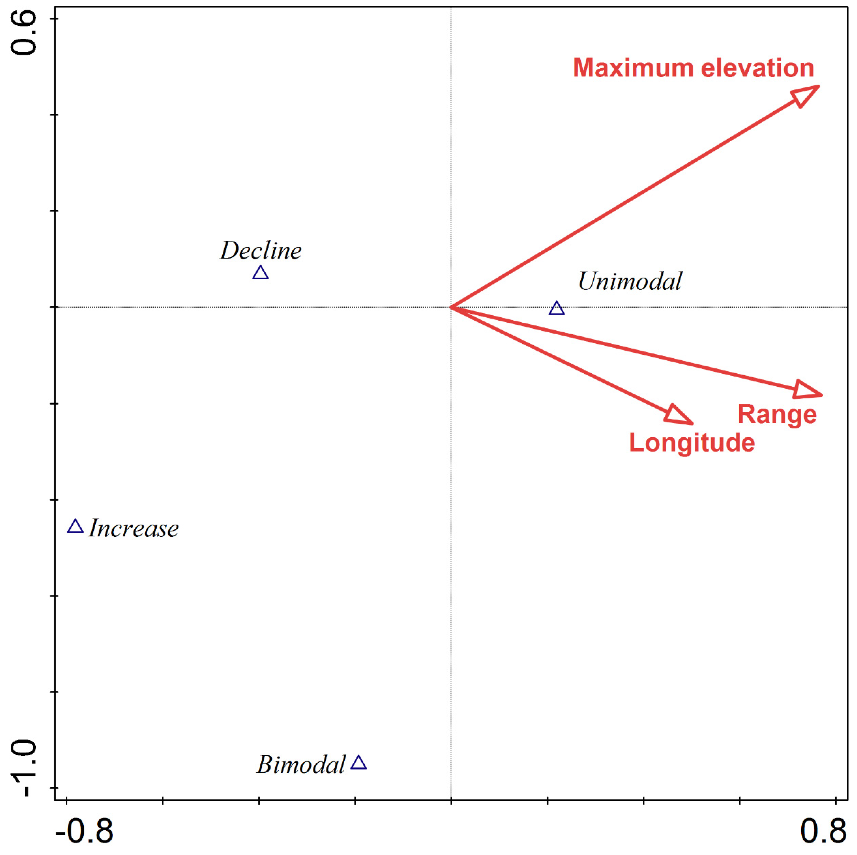
| Maximum elevation | 72.3 | 17.46 | 0.001 |
| Elevation range | 64.6 | 15.49 | 0.001 |
| Mean elevation | 23.3 | 5.35 | 0.001 |
| Longitude | 20.2 | 4.63 | 0.009 |
| Minimum elevation | 9.0 | 2.03 | 0.096 |
| Latitude | 3.5 | 0.80 | 0.476 |
| Taxonomy as covariable | |||
| Maximum elevation | 13.6 | 14.29 | 0.001 |
| Elevation range | 10.7 | 14.01 | 0.001 |
| Mean elevation | 9.0 | 5.48 | 0.040 |
| Longitude | 3.5 | 6.70 | 0.002 |
| Minimum elevation | 2.8 | 3.94 | 0.009 |
| Latitude | 0.9 | 1.07 | 0.339 |
Disclaimer/Publisher’s Note: The statements, opinions and data contained in all publications are solely those of the individual author(s) and contributor(s) and not of MDPI and/or the editor(s). MDPI and/or the editor(s) disclaim responsibility for any injury to people or property resulting from any ideas, methods, instructions or products referred to in the content. |
© 2025 by the authors. Licensee MDPI, Basel, Switzerland. This article is an open access article distributed under the terms and conditions of the Creative Commons Attribution (CC BY) license (https://creativecommons.org/licenses/by/4.0/).
Share and Cite
Irungbam, J.S.; Konvicka, M.; Fric, Z.F. Do Shapes of Altitudinal Species Richness Gradients Depend on the Vertical Range Studied? The Case of the Himalayas. Diversity 2025, 17, 215. https://doi.org/10.3390/d17030215
Irungbam JS, Konvicka M, Fric ZF. Do Shapes of Altitudinal Species Richness Gradients Depend on the Vertical Range Studied? The Case of the Himalayas. Diversity. 2025; 17(3):215. https://doi.org/10.3390/d17030215
Chicago/Turabian StyleIrungbam, Jatishwor Singh, Martin Konvicka, and Zdenek Faltynek Fric. 2025. "Do Shapes of Altitudinal Species Richness Gradients Depend on the Vertical Range Studied? The Case of the Himalayas" Diversity 17, no. 3: 215. https://doi.org/10.3390/d17030215
APA StyleIrungbam, J. S., Konvicka, M., & Fric, Z. F. (2025). Do Shapes of Altitudinal Species Richness Gradients Depend on the Vertical Range Studied? The Case of the Himalayas. Diversity, 17(3), 215. https://doi.org/10.3390/d17030215