Article

Modelling Urban Plant Diversity Along Environmental, Edaphic, and Climatic Gradients

by
Tuba Gül Doğan
1,*,
Engin Eroğlu
1,
Ecir Uğur Küçüksille
2,
Mustafa İsa Doğan
3 and
Tarık Gedik
4
1
Department of Landscape Architecture, Faculty of Forestry, Düzce University, 81620 Düzce, Türkiye
2
Department of Computer Engineering, Faculty of Engineering and Natural Sciences, Süleyman Demirel University, 32260 Isparta, Türkiye
3
Department of Industrial Engineering, Faculty of Engineering, Düzce University, 81620 Düzce, Türkiye
4
Department of Forest Industry Engineering, Faculty of Forestry, Düzce University, 81620 Düzce, Türkiye
*
Author to whom correspondence should be addressed.
Diversity 2025, 17(10), 706; https://doi.org/10.3390/d17100706 (registering DOI)
Submission received: 3 September 2025 / Revised: 5 October 2025 / Accepted: 7 October 2025 / Published: 13 October 2025
(This article belongs to the Section Plant Diversity)

Abstract

Urbanization imposes complex environmental gradients that threaten plant diversity and urban ecosystem integrity. Understanding the multifactorial drivers that govern species distribution in urban contexts is essential for biodiversity conservation and sustainable landscape planning. This study addresses this challenge by examining the environmental determinants of urban flora in a rapidly developing city. We integrated data from 397 floristic sampling sites and 13 environmental monitoring locations across Düzce, Türkiye. A multidimensional suite of environmental predictors—including microclimatic variables (soil temperature, moisture, light), edaphic properties (pH, EC (Electrical Conductivity), texture, carbonate content), precipitation chemistry (pH and major ions), macroclimatic parameters (CHELSA bioclimatic variables), and spatial metrics (elevation, proximity to urban and natural features)—was analyzed using nonlinear regression models and machine learning algorithms (RF (Random Forest), XGBoost, and SVR (Support Vector Regression)). Shannon diversity exhibited strong variation across land cover types, with the highest values in broad-leaved forests and pastures (>3.0) and lowest in construction and mining zones (<2.3). Species richness and evenness followed similar spatial trends. Evenness peaked in semi-natural habitats such as agricultural and riparian areas (~0.85). Random Forest outperformed other models in predictive accuracy. Elevation was the most influential predictor of Shannon diversity, while proximity to riparian zones best explained richness and evenness. Chloride concentrations in rainfall were also linked to species composition. When the models were recalibrated using only native species, they exhibited consistent patterns and maintained high predictive performance (Shannon R2 ≈ 0.937474; Richness R2 ≈ 0.855305; Evenness R2 ≈ 0.631796).

1. Introduction

Biodiversity, particularly plant species diversity and richness, constitutes a fundamental pillar of ecosystem functionality and resilience, directly influencing ecological stability, human well-being, and urban sustainability [1,2]. In the context of accelerating urbanization worldwide, understanding the multifaceted interactions between environmental variables and urban flora is critical for effective conservation and urban planning [3,4,5,6]. Urban ecosystems represent complex socio-ecological systems where anthropogenic pressures and environmental gradients converge, shaping the spatial distribution and community composition of plant species [7,8,9].
Extensive research has elucidated how microclimatic factors such as soil temperature, moisture, and light availability influence plant community structure and diversity in urban landscapes [10,11]. Soil properties including texture, pH, electrical conductivity, and organic matter content further modulate species distributions by affecting nutrient cycling and water retention [12,13]. Topographic factors were also influential. Moreover, precipitation chemistry—characterized by ion concentrations and pH variation—is an important yet underexplored determinant of urban vegetation health and diversity [14,15,16,17]. Macroclimatic indicators derived from bioclimatic variables additionally govern broader-scale patterns of species richness and community assembly [18,19,20]. Spatial landscape metrics—including proximity to forests, water bodies, roads, industrial zones, and urban centers—play a pivotal role in mediating seed dispersal, colonization, and anthropogenic disturbances, thereby influencing urban plant diversity gradients [6,21]. Despite recognition of these factors, research to date frequently addresses them in isolation or assumes linear relationships, inadequately capturing the complex, nonlinear interactions that govern urban plant diversity and community composition [22,23,24,25,26,27,28]. Particularly in rapidly urbanizing regions with heterogeneous landscapes, there remains a critical knowledge gap concerning how multiple environmental drivers collectively influence urban flora.
At the national scale, previous local studies have largely focused on floristic inventories or singular environmental drivers, lacking comprehensive, nonlinear modeling approaches that encompass multifactorial influences on urban plant diversity. Türkiye’s urban ecological research remains fragmented, with limited studies assessing the combined effects of microclimatic [29,30] edaphic, chemical, macroclimatic, and spatial factors on urban flora [31,32]. While there are studies examining urban flora generally, most of these lack direct measurements of environmental variables and rely on broad qualitative assessments rather than quantitative analyses [33]. Düzce, a rapidly urbanizing city with diverse topography and climatic conditions, represents an ideal natural laboratory to examine these interactions.
Addressing this critical research gap, the present study employs an integrative, multifactorial framework to quantify the relative contributions of microclimate (soil temperature, moisture, light availability), soil characteristics (texture, pH, (EC) electrical conductivity, organic matter), precipitation chemistry (monthly ion concentrations and pH), macroclimatic bioclimatic variables, and spatial landscape metrics (distance to forest, water bodies, roads, industrial areas, and urban centers) on plant species diversity, richness, and community composition within the urban matrix of Düzce. Utilizing advanced statistical modeling capable of capturing nonlinear interactions, this research aims to unravel the complex ecological processes shaping urban vegetation patterns. The core objective was to model each of indices (Shannon_H index, Richness, Evenness) separately using environmental predictors, identify the key determinants of diversity, and evaluate the predictive performance of different machine learning algorithms under a uniform analytical pipeline. In addition, to ensure the robustness of the findings, the analyses were also repeated exclusively with native species, enabling validation of whether the identified diversity–environment relationships hold when confined to the indigenous flora. The outcomes are expected to provide robust scientific insights for urban biodiversity conservation and inform climate-resilient, sustainable landscape management strategies tailored to mid-sized, rapidly transforming urban environments in Türkiye and analogous regions globally, particularly in the context of escalating climate change pressures.

2. Materials and Methods

2.1. Study Area

This study was conducted within the administrative boundaries of Düzce, a rapidly urbanizing mid-sized city located in northwestern Türkiye (40°50′ N, 31°09′ E). Situated within the western Black Sea ecoregion, Düzce lies in a transitional zone between the Euro-Siberian and Mediterranean floristic regions, supporting a heterogeneous mosaic of urban infrastructure, semi-natural green spaces, agricultural lands, and remnant forest patches. Covering an area of approximately 2574 km2, the province had a total population of 395,679 as of the end of 2021 [34]. Düzce was granted provincial status in 1999 following a major earthquake, which catalyzed significant infrastructural redevelopment and population influx, leading to fragmented and rapid urban expansion [35]. Düzce exhibits a geomorphologically diverse and ecologically significant topographical structure, characterized by a broad elevation range extending from near sea level in the northern lowland plains to approximately 1945 m in the Abant and Köroğlu mountain ranges to the south and east [36]. The provincial average elevation is around 500 m above sea level, reflecting a transitional landscape composed of coastal plains, alluvial basins, foothills, and densely forested uplands, representative of the Western Black Sea biogeographical zone. Notably, the city center is situated within a fertile intramontane basin at approximately 120–180 m elevation, encircled by forested mountain belts and high plateaus. This basin–mountain configuration not only governs the city’s hydrographic and climatic variability but also contributes to its ecological heterogeneity, supporting a mosaic of urban, agricultural, and semi-natural habitats with high floristic potential [37,38].
Düzce features a transitional climate between the Black Sea oceanic and inland continental types, characterized by relatively high precipitation and humidity, particularly in the spring and autumn months. The annual mean temperature is around 13.5 °C, while average annual precipitation exceeds 800 mm, supporting diverse vegetation types and land cover heterogeneity [39]. Düzce harbors a substantial diversity of both herbaceous and woody plant species, with a recorded flora comprising approximately 1700 taxa, of which nearly 10% are endemic to the region [40,41].

2.2. Vegetation Sampling

This study was conducted across a structured ecological gradient encompassing urban, suburban, and peri-urban zones within the study region. A total of 397 sampling points were established using a stratified random sampling approach across the urban matrix of Düzce (Figure 1). To achieve a confidence level of 90–95% with an acceptable margin of error (~5–10%) for estimating species richness and diversity patterns, we followed the sampling principles outlined by [42,43]. The required minimum sample size was calculated using standard ecological survey formulas, incorporating the assumed variance in Shannon diversity, the target confidence level, and the finite number of land-use in Düzce Province. This statistical justification validated our sample size of 397 sampling points. Plots that contained no vegetation or only a single plant species were excluded from further analysis, as such conditions do not provide ecologically meaningful data for capturing Shannon diversity patterns. In such cases, nearby sampling sites with comparable urbanization levels and greater floristic heterogeneity were selected as replacements. The sampling plots (n = 397) were systematically distributed across a diverse range of land cover categories defined by the CORINE classification system [44], encompassing urban, agricultural, forest, wetland, and riparian environments to ensure ecological representativeness (Table 1). The genesis of vegetation cover across the CORINE land-cover categories reflects distinct stages of anthropogenic transformation and functional reorganization of the territory. Continuous urban structures such as parks and designed green spaces represent planned vegetation intentionally established through landscaping practices. In contrast, discontinuous urban structures—including residential gardens, orchards, and urban voids—harbor mixed spontaneous and cultivated assemblages that signify transitional phases between managed and semi-natural vegetation. Industrial and transport-related areas support secondary plant communities that develop under recurrent disturbance, soil compaction, and modified hydrological conditions, while mining and construction sites exhibit early successional vegetation dominated by ruderal and pioneer species. These gradients collectively illustrate how shifts in land-use functionality influence vegetation genesis, structural heterogeneity, and the proportion of alien taxa within the urban ecological mosaic [45]. Although the number of plots varied across land cover categories due to logistical constraints, the analysis was designed to model plot-level alpha diversity metrics—including Shannon diversity (H′), species richness, and evenness—as a function of continuous environmental predictors. Since no categorical comparisons across habitat types were conducted, variation in plot numbers did not influence model validity or statistical structure.
Each vegetation plot was 20 × 20 m (400 m2), following standardized protocols for capturing urban plant diversity across life forms [46,47]. Within these plots, a nested sampling design was employed: woody vascular plant species were recorded across the full 400 m2, while shrub and herbaceous species were recorded within 5 × 5 m subplots placed centrally in each quadrat [24,48]. This hierarchical design balances representativeness with feasibility, especially in densely built-up areas where space and accessibility are constrained. It also reflects the structural layering of urban vegetation (Supplementary Materials Table S1), allowing for a detailed yet scalable assessment of biodiversity across urban–rural gradients.
The research material comprised herbaceous and woody plants from designated areas, collected based on key morphological traits such as flowers, fruits, cones, buds, leaves, stems, and roots. Habitat specificity was documented, and a dataset recorded the presence or absence of each species. The dried plant specimens were subsequently identified by experts from the Duzce University Faculty of Forestry Herbarium (DUOF). Cultivar identification was undertaken through systematic comparative analysis with authoritative horticultural and botanical references, including Botanica (the A–Z Encyclopedia of Garden Plants) [49], comprehensive landscape plant manuals, Türkiye’s Native and Exotic Trees and Shrubs I, II [50], and the national plant catalogs of Türkiye. For vegetation originating from parks, roadside plantings, or other public landscaping schemes, identifications were further corroborated using municipal planting plans and archival records. In the case of taxa widely employed in landscape practice, identification was facilitated by their high prevalence and the established familiarity of these species among experts. Taxon names were verified using the Global Biodiversity Information Facility (GBIF) [51] and the “Plants of the World Online” (POWO) [52] database. Presence data were used to calculate the Shannon diversity index (H′) as a measure of taxonomic diversity. Georeferenced plot locations were integrated with corresponding environmental datasets for spatial modeling.

2.3. Environmental Variables and Data Sources

To enhance analytical clarity, environmental predictors were grouped based on their origin into two categories: (i) field-derived measurements and (ii) secondary and geospatial data sources.

2.3.1. Field-Derived Environmental Variables

Environmental data were collected monthly over one year from 13 reference sites strategically selected to represent the environmental heterogeneity of the study area. These 13 reference sites were deliberately positioned to capture the full range of environmental variability across the study area—including differences in elevation, land cover types, proximity to urban and natural features, and topographic conditions—thereby ensuring representative spatial coverage for interpolating continuous environmental gradients. At each site, five replicate measurements of soil temperature, volumetric soil moisture, and photosynthetically active radiation (PAR) were obtained; mean values were used for modeling. Light availability was treated as a microclimatic variable reflecting local canopy openness and solar radiation conditions that influence site-level energy balance. Atmospheric deposition was sampled using passive rain collectors, and monthly precipitation was analyzed in the laboratory for pH, electrical conductivity (EC), and concentrations of CO32−, HCO3, Cl, SO42−, Ca2+, K+, Mg2+, and Na+. In addition, composite soil samples were collected from a depth of 0–30 cm at each of the 397 plots and analyzed for pH, EC, organic matter content, texture, and carbonate concentration. All site-specific values were spatially interpolated using ordinary Kriging (ArcGIS 10.3), and interpolated surfaces were resampled to the floristic plots using the ‘Extract Multi Values to Points’ tool.

2.3.2. Secondary and Geospatial Data Sources

Nineteen bioclimatic variables (BIO1–BIO19) were retrieved from the CHELSA database at a spatial resolution of 30 arc-seconds. Contemporary meteorological data, including monthly means of air temperature, relative humidity, and total precipitation, were acquired from the Turkish State Meteorological Service (TSMS). Spatial metrics such as distance to forest edges, water bodies, roads, industrial zones, and the urban core were calculated using Euclidean distance functions in GIS. Additional topographic predictors, including slope, aspect, terrain ruggedness index (TRI), and topographic position index (TPI). Topographic variables were derived from the ALOS PALSAR Digital Elevation Model (DEM).
To ensure terminological consistency and facilitate the interpretation of model outputs, each environmental variable was assigned a standardized abbreviation. These codes were used uniformly throughout the modeling process, figures, and statistical evaluations. Table 2 summarizes the full list of environmental predictors along with their respective abbreviations and descriptions.

2.4. Statistical Analyses

2.4.1. Dataset and Diversity Metrics

Field-based floristic surveys were conducted across sampling sites within the urban matrix to document vascular plant species. All observed taxa were taxonomically verified using national floras and cross-checked with current nomenclature. For each sampling site, three widely accepted biodiversity metrics were computed: the Shannon Diversity Index (H′), species richness (S), and Pielou’s evenness index (J′). Shannon Diversity Index was used as the primary diversity metric, while Species Richness and Evenness were included as structural components of community composition to further dissect patterns of floristic organization.
These metrics were derived from the plant species lists obtained per site and served as response variables in subsequent modeling. Calculations were performed using the scikit-bio package in Python 3.10: skbio.diversity.alpha.shannon() for Shannon diversity, observed_otus() for species richness, and a custom computation for evenness (J′ = H′/ln (S)). H′ values typically range from 1.5 to 3.5 in ecological studies, where values above 3.0 indicate highly diverse and evenly distributed plant communities, while values near or below 2.0 suggest lower diversity with dominance by a few species, often reflecting environmental stress or anthropogenic disturbance [53]. In addition to floristic data, each sampling site was characterized by a suite of climatic, ecological, edaphic, and topographic predictors. All explanatory variables were compiled into a unified dataset for further preprocessing and modeling.
In addition to diversity indices, the proportion of native species was calculated for each sampling plot to examine potential compositional effects on diversity–environment relationships. For each plot, native species proportion was calculated as the number of native species divided by the total number of species recorded. A Random Forest regression model was applied to identify environmental predictors of native species proportion, using the same predictor set employed in the diversity models.
To assess the robustness of the diversity–environment relationships, we repeated the computation of Shannon diversity (H′), species richness (S), and Pielou’s evenness (J′) after filtering each plot’s species list to native taxa only. Species origin (native vs. non-native) was curated from regional floras and global databases consistent with the taxonomy control used in the main analysis; both spontaneously occurring and planted natives were retained as “native,” whereas all non-native taxa (whether spontaneous or cultivated) were exclude [1,3,5]. Metrics were computed identically to the primary analysis.

2.4.2. Feature Preprocessing and Multicollinearity Control

To enhance model reliability and interpretability, all numerical predictors were subjected to a structured three-step preprocessing procedure (Table 3). First, z-score standardization was applied to normalize variables across differing units and scales, reducing the influence of extreme values while ensuring numerical stability in algorithms sensitive to feature magnitudes. Second, pairwise Pearson correlation analysis was conducted to remove highly collinear variables (|ρ | > 0.85), thereby minimizing redundancy. Finally, Variance Inflation Factor (VIF) analysis was performed iteratively, and predictors with VIF scores exceeding 10 (VIF > 10) were excluded to mitigate multicollinearity and stabilize variance estimates [54,55].

2.4.3. Model Development and Variable Importance Analysis

To model the relationships between biodiversity metrics and environmental predictors, three separate machine learning regression models were implemented for each diversity index: Random Forest (RF), Extreme Gradient Boosting (XGBoost), and Support Vector Regression (SVR) with a radial basis function (RBF) kernel. All models were trained using an 80:20 train-test split, with the random state set to 42 to ensure reproducibility. No stratification was applied due to the continuous nature of the response variables.
RF regression was employed as the primary modeling approach for each biodiversity metric—Shannon diversity, species richness, and evenness—using the refined predictor set. The model ensemble comprised 500 trees with bootstrapped sampling and randomized feature splits. RF was chosen for its ability to capture complex nonlinear relationships without parametric assumptions and its robustness to outliers.
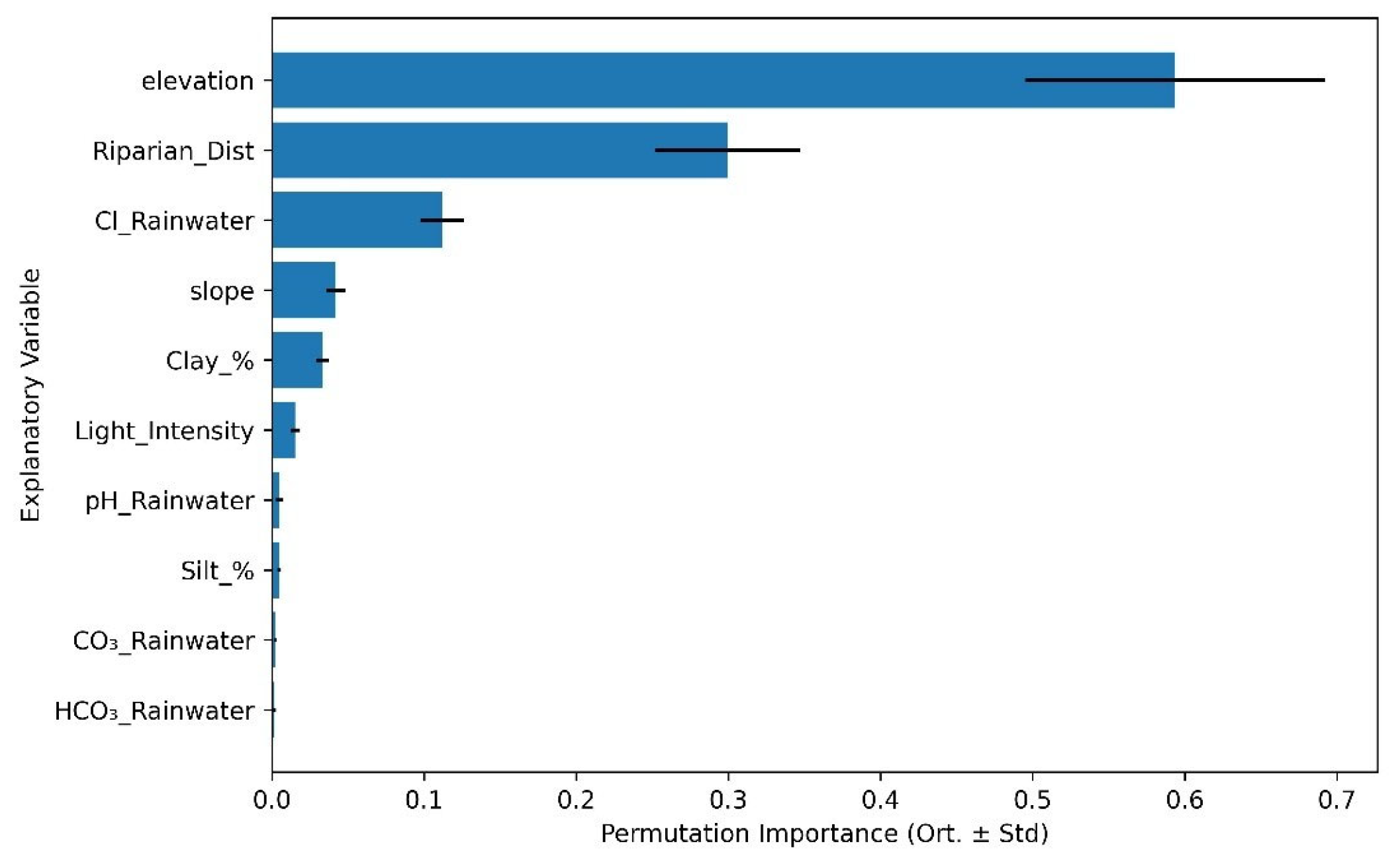
Permutation importance analysis was conducted on the test set by randomly shuffling each predictor and measuring the resulting decline in R2, yielding an unbiased estimate of variable influence. Consistently across models, key predictors included elevation, forest distance, slope, and soil moisture-related variables such as field capacity and texture components.

2.4.4. Comparative Model Evaluation

Model performance was assessed on the held-out test set using four standard evaluation metrics: the coefficient of determination (R2), mean absolute error (MAE), mean squared error (MSE), and root mean square error (RMSE). These metrics were chosen to reflect both goodness-of-fit and error dispersion, providing a comprehensive performance profile for each model (Table 4).
To ensure a fair benchmark, all models were trained and tested under identical conditions using the same 10 predictors and data partitions. Among the tested models, Random Forest consistently outperformed XGBoost and SVR across all biodiversity indices. Therefore, only the results and interpretation from the RF model were retained for subsequent analysis and discussion.

2.4.5. Permutation-Based Variable Importance

Following model training, permutation importance analysis was conducted on the Random Forest model to quantify the relative influence of each predictor. For each variable, its values were randomly permuted in the test set, and the corresponding drop in R2 was recorded. This process was repeated over 10 Monte Carlo iterations, and the average decrease in performance was used as an estimate of variable importance.

2.4.6. Spatial Autocorrelation Testing

To assess the independence of model residuals, Moran’s I tests [56] were conducted for each diversity metric (Shannon H′, species richness, and evenness). Residuals were derived from the best-performing model for each metric and spatially joined to plot coordinates. Spatial autocorrelation was tested using the permutation-based global Moran’s I method with 999 Monte Carlo simulations, implemented in Python’s ‘esda’ module. This step was critical to confirm that the residuals did not exhibit spatial dependence, thereby ensuring the robustness of model generalizability.

2.4.7. Model Validation and Generalization Testing

To assess the generalizability and robustness of the Random Forest models applied for predicting Shannon diversity, species richness, and evenness, we implemented several cross-validation (CV) and replication techniques. First, we conducted a repeated 10-fold cross-validation [57] with 5 repetitions, which allowed for estimating model performance variability across multiple data partitions. Second, a 50-replicate hold-out validation was applied by randomly splitting the dataset into training (80%) and testing (20%) sets, repeated 50 times to capture prediction stability. Finally, to ensure that the model’s predictive power was not the result of chance, a Y-randomization test (permutation test) was conducted by randomly shuffling the response variable and re-training the model, generating a null distribution of R2 values for comparison [58]. All validation procedures and visual diagnostics, including predicted vs. observed parity plots and residual distribution analyses, were performed in Python. The scikit-learn library was used for cross-validation, model training, and performance evaluation. Data manipulation and statistical computations were conducted using numpy and pandas, while model diagnostics and validation plots were generated using matplotlib and seaborn.

3. Results

Field investigations across 397 sampling sites led to the identification of 763 taxa distributed among diverse CORINE land cover types (The full taxa-by-plot presence–absence matrix is provided as Supplementary Materials Table S1). This extensive dataset facilitated a robust analysis of species diversity, richness, and evenness patterns relative to land cover classification. The proportion of native species exceeded 70% in 95.7% of the sampling plots, with only 4.3% of plots showing values below 50%.
Species diversity, quantified via the Shannon Diversity Index, exhibited marked heterogeneity across the different land cover categories. Broad-leaved forests and pasture areas consistently displayed elevated diversity values, frequently exceeding 3.0, indicative of their complex community assemblages. Conversely, urban fabric zones, encompassing both continuous and discontinuous urban areas, recorded mean Shannon index values near 2.3, reflecting reduced heterogeneity. The lowest diversity indices, often below 2.3, were associated with construction sites and mining areas, underscoring the impact of intensive anthropogenic disturbance on floristic variety (Figure 2).
Species richness patterns (Figure 3) closely mirror those of diversity, with natural habitats such as broad-leaved forests and pastures harboring the greatest number of species. Urbanized and heavily modified landscapes (İndustrial landscapes, Mining zones) demonstrated markedly reduced species richness, emphasizing the critical role of habitat quality and human disturbance in shaping plant community composition.
Evenness, representing species distribution uniformity (Figure 4), demonstrated comparatively lower variability but revealed important trends. Highest evenness values, approaching 0.85, were found in semi-natural habitats including mixed agricultural zones and watercourse areas. In contrast, urban fabrics and heavily altered sites exhibited evenness indices ranging from 0.55 to 0.65, consistent with communities dominated by fewer species. Variance within groups for diversity and richness was notably elevated in broad-leaved forests and pasturelands, reflecting high site-to-site heterogeneity, while evenness values showed comparatively less within-group variability.
Analysis of confidence intervals for Shannon diversity and species richness revealed substantial overlap among several natural habitat categories, particularly among forest types and pasture areas. Urban and modified land covers, however, consistently formed distinct clusters characterized by significantly lower biodiversity metrics. Furthermore, the dispersion of individual observations indicated a wider spread in natural and semi-natural habitats, while urban and industrial land covers displayed tighter data clustering around reduced mean values.
Permutation importance analysis revealed distinct but overlapping sets of environmental drivers for each metric. For Shannon Diversity (Figure 5), the most influential predictors were elevation (importance = 0.594 ± 0.099), distance to water bodies (0.300 ± 0.048), and chloride concentration in rainfall (0.112 ± 0.014), followed by slope (0.042 ± 0.006), percent clay (0.033 ± 0.004), and light availability (0.015 ± 0.003). Minor contributions were observed for pH (0.005 ± 0.002), silt percentage (0.005 ± 0.001), carbonate (CO32−) (0.002 ± 0.001), and bicarbonate (HCO3) (0.002 ± 0.001).
In the case of Species Richness, distance to riparian zones emerged as the dominant predictor (importance > 1.0), substantially surpassing all other variables. Secondary contributors included distance to industrial areas, distance to urban centers, and elevation, while edaphic and climatic parameters had comparatively limited influence (Figure 6). This outcome underscores the critical role of hydrological connectivity in shaping species accumulation patterns in urban landscapes.
For Evenness, model predictions were driven by a more nuanced combination of environmental factors. Distance to riparian zone again ranked highest in importance (0.36 ± std), followed by chloride concentration in rainfall, light availability, and elevation. Notably, the reduced effect sizes and slightly lower R2 suggest that evenness is less directly structured by macro-environmental variables than species richness or overall diversity, potentially reflecting more localized microhabitat effects and species dominance dynamics (Figure 7).
Permutation importance analysis repeated with native taxa-only data produced broadly consistent results. The same top three predictors—elevation, proximity to riparian zones, and chloride concentration in rainfall—retained the highest explanatory power across Shannon diversity, richness, and evenness models. Minor shifts were observed in lower-ranked predictors (e.g., clay %, slope, light intensity), but these did not alter the overall explanatory structure. Detailed ranked importance values are provided in the Supplementary Materials Table S2.
Following multicollinearity screening via VIF analysis, five bioclimatic variables (BIO1, BIO4, BIO9, BIO12, and BIO15) were retained in the final predictor set. While these variables were included in all models, their relative importance varied across diversity metrics. Notably, BIO9 and BIO12 contributed moderately to the richness model, while BIO12 and BIO15 were similarly ranked in the evenness model. In the Shannon diversity model, no bioclimatic variable ranked among the top predictors.
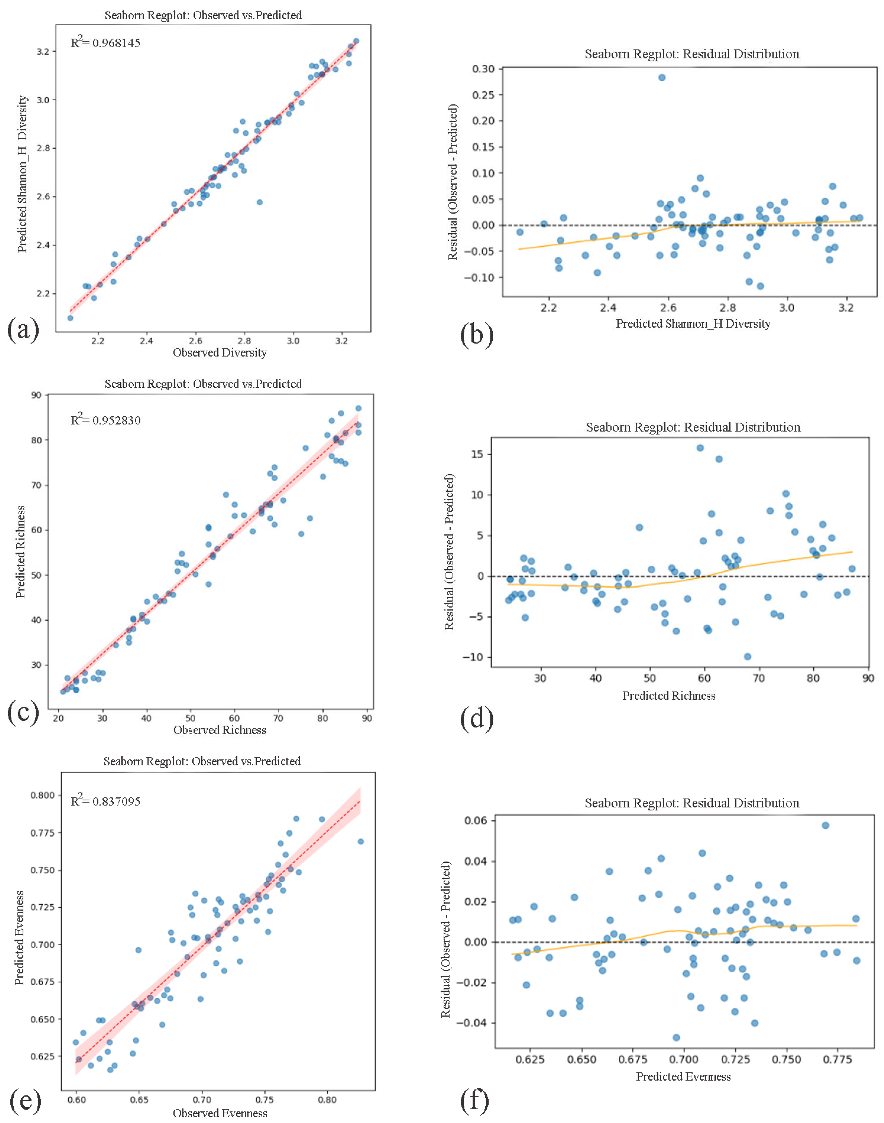
Among the applied models, RF regression demonstrated robust explanatory performance across the primary diversity index (Shannon_H′ Diversity) and two key structural components of community composition—Species Richness and Evenness—when evaluated along urban environmental gradients. Each model yielded high predictive accuracy, with R2 values for Shannon, Richness, and Evenness. Predicted and observed values showed strong linear correspondence in all three cases, and residuals were symmetrically distributed around zero without detectable bias or heteroscedasticity, indicating reliable and consistent model behavior across varying urban ecological contexts (Figure 8).
When restricted to native species, Random Forest remained the best-performing model for predicting species richness and evenness, whereas XGBoost yielded the highest predictive accuracy for Shannon diversity. Observed vs. predicted relationships and residual distributions for these native-only models are presented in Figure 9.
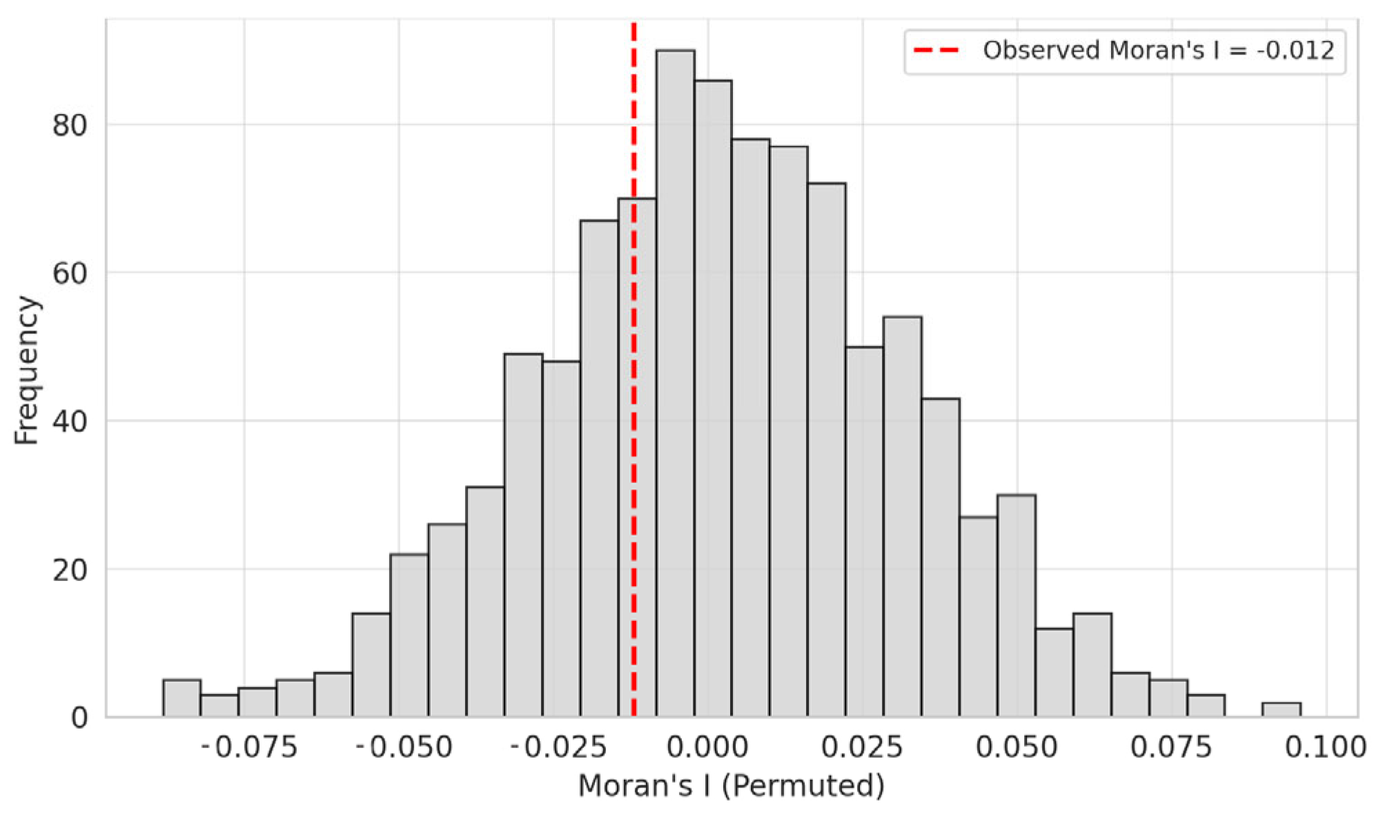
To verify the spatial independence of model residuals, Moran’s I statistic was computed for the RF model predicting Shannon diversity (H′). The test revealed no significant spatial autocorrelation among the residuals (Moran’s I = −0.012, p = 0.302), indicating that the model adequately captured the spatial structure of the predictors and that residuals were randomly distributed within the study area (Figure 10). This suggests that the model results are not biased by spatial clustering effects and can be considered spatially robust.
Additionally, Moran’s I statistics were also calculated for the residuals of the RF models predicting species richness and evenness, respectively. For Species Richness, Moran’s I was –0.015 (p = 0.277), and for Evenness, Moran’s I was –0.018 (p = 0.246), both indicating no significant spatial autocorrelation. These findings support the spatial robustness of all diversity models and suggest that residuals were randomly distributed across the study area, confirming that the spatial structure of predictors was adequately captured by the models.
To evaluate the generalizability and predictive strength of the RF models, a suite of robust validation techniques was applied across all three biodiversity metrics. As summarized in Table 5, the RF models yielded consistently high performance, with Shannon diversity showing the strongest predictive capacity (mean CV R2 = 0.968), followed by species richness (CV R2 = 0.948) and evenness (CV R2 = 0.858). These results indicate that environmental, edaphic, and climatic predictors collectively explained a substantial proportion of the observed variability. Repeated 10-fold cross-validation with five iterations revealed low error margins (e.g., CV RMSE = 0.047 for Shannon), and this reliability was corroborated by out-of-fold (OOF) and repeated hold-out validation tests, both of which produced R2 and RMSE values in close agreement with cross-validation results. Additionally, the Y-randomization test resulted in near-zero or negative R2 values across all three indices, confirming that the models did not overfit and that the performance was not due to chance structure in the data. These validation outcomes underscore the robustness and generalizability of the RF approach for modeling complex biodiversity–environment relationships in urban ecological contexts.
The model for Shannon diversity exhibited robust predictive capacity with a 10-fold cross-validation R2 of 0.968 ± 0.014 and RMSE of 0.047 ± 0.010. Out-of-fold predictions further confirmed the model’s stability (R2 = 0.970; RMSE = 0.047). The hold-out validation repeated 50 times yielded consistent results (R2 = 0.966 ± 0.012), demonstrating high generalizability across random data partitions (Figure 11a). Finally, the Y-randomization test yielded a near-zero R2 distribution (mean R2 = −0.181), strongly indicating that model performance was not due to overfitting or spurious correlation (Figure 11b). Similar validation results were observed for species richness and evenness, with both metrics exhibiting high R2 and low RMSE across all validation strategies. The Y-shuffle tests for these indices also produced R2 values close to zero, reinforcing the reliability of the models.
For the native-only analyses, cross-validation and Y-randomization diagnostics produced highly comparable outcomes, with similarly high R2 and low RMSE values across all indices. Y-shuffle tests again yielded near-zero R2 distributions, confirming that the predictive performance observed for native species was not due to overfitting or spurious correlation.

4. Discussion

This study demonstrates that urban plant diversity in a mid-sized, rapidly urbanizing city is not random, but shaped by a complex interplay of environmental filters operating at multiple spatial and functional scales. Among predictors, elevation emerged as the dominant driver of Shannon diversity, reflecting the influence of altitudinal gradients on microclimatic stability, habitat heterogeneity, and ecological niche availability [59,60]. Elevated zones in Düzce likely provided cooler, moister conditions, supporting taxonomic richness in line with patterns observed in montane and transitional landscapes [25,28].
Interestingly, mixed forest areas (CORINE 3.1.3) demonstrated lower-than-expected levels of species richness and diversity, occasionally even trailing highly disturbed environments such as mining zones. Field observations also revealed that, although these forests featured sparse tree canopies dominated by coniferous species, the understory vegetation was remarkably poor. This may be attributed not only to abiotic constraints but also to the limited ecological complementarity and functional overlap among present species, which hinders the formation of structurally and compositionally diverse plant layers. The lack of a developed shrub and herbaceous stratum restricts vertical complexity and reduces the potential for interspecific facilitation or niche partitioning, thereby resulting in simplified and loosely assembled communities [61]. In contrast, mining areas supported early-successional plant communities dominated by ruderal, opportunistic, and often invasive species. These species rapidly colonize degraded substrates, taking advantage of low competition, high light availability, and abundant seed rain from surrounding habitats. While such conditions may temporarily boost species richness, they often reflect unstable community structures that are vulnerable to rapid turnover as succession progresses or human disturbance intensifies [62,63]. Hence, interpreting high richness in such contexts requires ecological caution, as it may not indicate long-term ecosystem stability. Moreover, it is important to note that the current study does not aim to directly compare different land-cover types. A valid habitat-type comparison would require balanced sampling across all CORINE classes and the use of beta diversity indices to quantify species turnover between habitat types [64]. Our design focused instead on detecting gradual spatial shifts in floristic diversity along an urban–rural environmental gradient, with land-cover categories considered as contextual layers rather than as categorical explanatory variables.
Proximity to water bodies emerged as a key determinant of Shannon diversity, Richness and Evenness, suggesting the critical role of hydrological features in sustaining species-rich assemblages. Riparian zones, in particular, have long been recognized as biodiversity hotspots due to their microclimatic buffering, structural heterogeneity, and connectivity functions [65,66]. Our findings reinforce their significance within fragmented urban environments, where such habitats may serve as refugia or dispersal corridors. Precipitation chemistry variables, notably chloride ion concentration and pH, were also significantly associated with diversity metrics, underscoring the growing recognition of atmospheric deposition as an influential ecological stressor in urban ecosystems [14,15,67]. Elevated chloride levels may reflect anthropogenic pollution sources such as road salting and industrial emissions, which can alter soil chemistry and inhibit sensitive taxa [25]. The measurable impact of ion concentrations and rainfall pH on species composition supports calls for integrating atmospheric monitoring into urban ecological assessments. Edaphic parameters such as percent clay and slope had moderate but notable effects on diversity. Clay-rich soils can retain more nutrients and water but may also reduce aeration, affecting root dynamics and species sorting [68]. Slope influences runoff, soil erosion, and exposure, thereby shaping microhabitats and plant strategies [22]. These findings mirror similar results in other urban landscape ecology studies, emphasizing that physical terrain remains a key structuring force even amid urban anthropogenic overlays.
Unlike Shannon diversity, species richness was most strongly shaped by distance to riparian zones, reaffirming the pivotal ecological function of water-adjacent corridors in urban environments [69]. These features likely facilitate seed dispersal, act as refugia, and enhance beta-diversity by linking habitat patches [21,26]. Furthermore, the proximity to industrial zones and urban cores exhibited negative effects, reflecting biotic homogenization trends and species loss under high anthropogenic pressure [4,23].
Evenness, though often neglected in urban biodiversity assessments, provides valuable insight into community dominance structures. Our results show that evenness is moderately influenced by light availability, riparian proximity, and chloride ion concentration, suggesting that resource competition and localized disturbances shape community equilibrium [10]. The lower explanatory power of environmental variables on evenness further implies the influence of biotic interactions, land-use history, or unmeasured microhabitat characteristics. This highlights the need for future studies to integrate functional traits or disturbance regime data to better predict dominance hierarchies in urban vegetation.
From a methodological standpoint, the superior performance of the RF model across all biodiversity indices confirms its utility in ecological studies involving high-dimensional, nonlinear data structures [70]. Its capacity to uncover complex variable interactions without a priori assumptions provides robust insights into the multifactorial nature of urban biodiversity drivers. The observed alignment between predicted and actual values, along with the residuals’ normal and patternless distribution, affirms both model reliability and spatial generalizability, particularly within urban ecological applications [70,71]. The overall consistency between the model performance metrics and spatial diagnostics further validates the robustness of our predictions. The Moran’s I test on model residuals revealed no significant spatial autocorrelation, confirming that the residuals were spatially random [56]. This dual confirmation—high explanatory power (R2) and the absence of spatial autocorrelation in residuals—indicates both predictive strength and spatial robustness of the model, as advocated in spatial machine learning literature [72,73].
Permutation-importance profiles derived from the native-only analyses converged strongly with those from the full dataset, as elevation, riparian proximity, and chloride concentrations in rainfall consistently emerged as dominant predictors across diversity indices, while only minor shifts occurred among lower-ranked variables (e.g., clay content, slope, light availability). This stability underscores the robustness of the identified environmental drivers and corroborates the view that edaphic–hydrological gradients remain central in structuring plant diversity even under anthropogenic pressure [5,21]. From a methodological perspective, model performance patterns were also broadly concordant: Random Forest retained superior predictive power for species richness and evenness, whereas XGBoost yielded the highest accuracy for Shannon diversity when restricted to native taxa. Such algorithm-specific variation is not unexpected, as ensemble tree-based learners differ in their capacity to capture feature interactions and nonlinearities [70,74,75]. Comparable findings in ecological modeling have highlighted that Random Forest tends to excel in multi-collinear settings, whereas gradient boosting frameworks can better exploit dominant hierarchical effects within predictors [71,76]. Collectively, these outcomes indicate that the primary ecological gradients shaping urban floristic diversity are resilient to the inclusion or exclusion of non-native species, thereby reinforcing the ecological validity and methodological generalizability of the present study.
Contrary to the general assumption that alien or adventitious species exhibit stronger and more differentiated associations with environmental factors than native taxa [77,78], the present findings indicate that native flora still dominates the ecological structure across the urban–rural matrix of Düzce. The proportion of native species exceeding 70% in nearly all sampling plots suggests that anthropogenic transformation has not yet led to a pronounced ecological homogenization or replacement by alien elements [4,25]. This pattern likely reflects the buffering capacity of the city’s heterogeneous landscape mosaic—where topographic variation, remnant forest patches, and riparian corridors maintain stable microhabitats that favor the persistence of native assemblages [3,79]. While adventitious species are indeed known to preferentially colonize ecotopes with high environmental heterogeneity or recurrent disturbance [80], their relatively limited representation in Düzce indicates that current urbanization processes have primarily altered species abundance and dominance structures rather than fundamentally reshaped floristic composition. Therefore, the observed dominance of native taxa aligns only partially with the hypothesis proposed by [79] as alien species may respond more strongly to environmental heterogeneity in highly disturbed urban contexts, whereas such dynamics remain subdued in moderately transformed landscapes like Düzce. Collectively, these findings highlight that the relationship between alien taxa and environmental factors is context-dependent, intensifying only beyond specific thresholds of disturbance and ecological simplification.
The analysis of species origin revealed a consistently high dominance of native taxa across the urban–rural gradient, with native species comprising over 70% of the total species pool in the vast majority of plots. This finding directly addresses the concern that mixing wild and cultivated taxa could compromise ecological specificity by masking true environmental gradients. In our study system, the persistence of native dominance despite urbanization aligns with evidence from other regions showing that when regional species pools remain intact, urban floras can retain a high proportion of indigenous elements even under substantial anthropogenic pressures [6,81]. Therefore, the strong explanatory relationships identified between diversity metrics and environmental predictors can be interpreted as robust reflections of ecological processes rather than artifacts of uneven representation of native versus non-native taxa.
Although this study includes managed and human-influenced sites such as urban parks and residential areas, these landscapes remain ecologically relevant within the scope of urban ecology. The coexistence of spontaneous and intentionally planted species is a defining feature of urban vegetation and reflects the complex socio-ecological fabric of cities [3,6,82]. Notably, key environmental drivers—such as soil pH, salinity, light, and microclimate—continue to shape species assembly even in anthropogenically modified habitats [24,83]. While this study focused on capturing broad-scale patterns in plant diversity along an urban–rural gradient, future research could consider stratifying urban land-use types based on socioeconomic characteristics (e.g., income level, education, or management practices within residential zones). Such approaches may complement landscape-scale insights with finer-grained socio-ecological understanding.
This result is consistent with several ecological modeling studies where RF has demonstrated superior performance in capturing the hierarchical and nonlinear effects of multiple predictors on species diversity and distribution [84,85]. For instance, RF has been successfully applied to urban and peri-urban floristic data to resolve complex interactions between anthropogenic gradients and biodiversity outcomes, often outperforming traditional linear or parametric models [86,87]. Importantly, while some literature raises concerns about RF’s stability under small or imbalanced datasets [85,88], our model’s strong predictive capacity, combined with the absence of spatial autocorrelation in the residuals (Moran’s I results), affirms both its accuracy and spatial robustness in our case. Moreover, our findings contribute to a growing body of evidence supporting the use of RF in urban biodiversity assessments, particularly in heterogeneous landscapes where vegetation patterns are shaped by both environmental filters and human intervention [89]. The capacity of RF to handle multicollinearity, nonlinear responses, and interaction terms without overfitting is especially valuable in such settings. Taken together, these results validate the methodological soundness of our model choice and support its relevance for future ecological modeling frameworks in complex urban contexts. The consistently high predictive performance of the RF model across all diversity metrics (Shannon, richness, and evenness), as confirmed by repeated cross-validation, hold-out, and permutation tests, underscores the methodological robustness of our approach and highlights its potential applicability in future urban biodiversity modeling efforts.

5. Conclusions

This study, by integrating a comprehensive suite of environmental predictors—including microclimatic, edaphic, precipitation chemistry, macroclimatic, and spatial landscape metrics—and applying nonlinear machine learning models, this study identified the multifactorial drivers shaping urban plant diversity across a heterogeneous ecological matrix. Among the tested algorithms (RF, XGBoost, SVR) the RF regression model consistently demonstrated superior predictive performance across all diversity indices, confirming its suitability for modeling complex, nonlinear ecological interactions. In the native-only validation analyses, Random Forest likewise remained the top performer for richness and evenness, whereas XGBoost provided the best predictive accuracy for Shannon diversity, underscoring the methodological robustness and complementarity of ensemble tree-based approaches. Elevation emerged as the most influential predictor of Shannon diversity, highlighting the pivotal role of topographic heterogeneity and microclimatic stability in sustaining diverse plant assemblages—factors that are increasingly critical under the accelerating impacts of climate change. In contrast, species richness and evenness were primarily structured by proximity to riparian zones, underscoring the ecological significance of hydrological corridors in enhancing habitat connectivity and buffering against urban stressors, including those intensified by shifting climatic regimes. Additionally, the influence of chloride concentrations in precipitation suggests that atmospheric deposition may exert a subtle but measurable pressure on community composition within urban ecosystems. Collectively, these findings emphasize the necessity of incorporating spatially explicit and multidimensional environmental data into biodiversity assessments and advocate for the conservation of elevational gradients and riparian interfaces as core components of climate-resilient urban green infrastructure planning. The modeling framework presented here offers a transferable approach for urban ecological diagnostics and supports evidence-based strategies to enhance biodiversity resilience in rapidly urbanizing regions. Future research should incorporate functional trait data and socioecological monitoring to better capture the temporal and biotic complexities of urban plant diversity dynamics.

Supplementary Materials

The following supporting information can be downloaded at https://www.mdpi.com/article/10.3390/d17100706/s1, Table S1: Presence–absence matrix of plant species across CORINE Land Cover Codes. Each “x” indicates the occurrence of a species within a given CORINE land-cover type; Table S2: Top ten predictors of Shannon diversity (H′), species richness (S), and evenness (J′) based on permutation importance in models restricted to native species.

Author Contributions

Conceptualization, T.G.D. and E.E.; methodology, T.G.D., E.E. and E.U.K.; software, T.G.D. and E.U.K.; validation, E.U.K.; formal analysis, T.G.D. and E.U.K.; investigation, T.G.D. and E.E.; resources, T.G.D. and E.E.; data curation, T.G.D.; writing—original draft preparation, T.G.D.; writing—review and editing, T.G.D., E.E., E.U.K., M.İ.D. and T.G.; visualization, T.G.D. and E.U.K.; supervision, E.E., M.İ.D. and T.G.; project administration, T.G.D. and E.E. All authors have read and agreed to the published version of the manuscript.

Funding

This study is supported by TÜBİTAK 1002-A Project No: 124O656.

Data Availability Statement

A complete list of all plant species identified per sampling plot is provided in Supplementary Materials Table S1.

Acknowledgments

This study is supported by 124O656 ‘The Influence of Environmental Variables on the Distribution and Prediction of Urban Flora Supported by Nonlinear Regression Models and Machine Learning’ Project (TÜBİTAK 1002-A). We would like to thank TÜBİTAK, project managers and teams: TÜBİTAK 2237—Determination of Biological Diversity Based on Species, Taxonomic, Functional, and Structural Characteristics. TÜBİTAK 2237—Nature-Science-Based Exploratory Data Analysis and Data Visualization. This article is derived from the doctoral dissertation of the first author (Tuba Gül Doğan), conducted at Düzce University, Department of Landscape Architecture under the supervision of Engin Eroğlu.

Conflicts of Interest

The authors declare no conflicts of interest.

Abbreviations

The following abbreviations are used in this manuscript:
RFRandom Forest
XGBoostExtreme Gradient Boosting
SVRSupport Vector Regression
DUOFDuzce University Faculty of Forestry Herbarium
GBIFGlobal Biodiversity Information Facility
POWOPlants of the World Online
ECElectrical conductivity
VIFVariance Inflation Factor

References

  1. Gaston, K.J. Urban Ecology; Cambridge University Press: Cambridge, UK, 2010. [Google Scholar] [CrossRef]
  2. Cardinale, B.J.; Duffy, J.E.; Gonzalez, A.; Hooper, D.U.; Perrings, C.; Venail, P.; Narwani, A.; Mace, G.M.; Tilman, D.; Wardle, D.A.; et al. Biodiversity loss and its impact on humanity. Nature 2012, 486, 59–67. [Google Scholar] [CrossRef]
  3. Aronson, M.F.J.; La Sorte, F.A.; Nilon, C.H.; Katti, M.; Goddard, M.A.; Lepczyk, C.A.; Warren, P.S.; Williams, N.S.G.; Clilliers, S.; Clarkson, B.; et al. A global analysis of the impacts of urbanization on bird and plant diversity reveals key anthropogenic drivers. Proc. R. Soc. B Biol. Sci. 2014, 281, 20133330. [Google Scholar] [CrossRef]
  4. Mckinney, M. Urbanization as a major cause of biotic homogenization. Biol. Conserv. 2006, 127, 247–260. [Google Scholar] [CrossRef]
  5. Aronson, M.F.J.; Handel, S.N.; La Puma, I.P.; Clemants, S.E. Urbanization promotes non-native woody species and diverse plant assemblages in the New York metropolitan region. Urban Ecosyst. 2015, 18, 31–45. [Google Scholar] [CrossRef]
  6. Kowarik, I. Novel urban ecosystems, biodiversity, and conservation. Environ. Pollut. 2011, 159, 1974–1983. [Google Scholar] [CrossRef] [PubMed]
  7. Mckinney, M. Effects of urbanization on species richness: A review of plants and animals. Urban Ecosyst. 2008, 11, 161–176. [Google Scholar] [CrossRef]
  8. McDonald, R.I.; Mansur, A.V.; Ascensão, F.; Colbert, M.; Crossman, K.; Elmqvist, T.; Gonzalez, A.; Güneralp, B.; Haase, D.; Hamann, M.; et al. Research gaps in knowledge of the impact of urban growth on biodiversity. Nat. Sustain. 2019, 3, 16–24. [Google Scholar] [CrossRef]
  9. Seto, K.C.; Güneralp, B.; Hutyra, L.R. Global forecasts of urban expansion to 2030 and direct impacts on biodiversity and carbon pools. Proc. Natl. Acad. Sci. USA 2012, 109, 16083–16088. [Google Scholar] [CrossRef]
  10. Shochat, E.; Warren, P.S.; Faeth, S.H.; McIntyre, N.E.; Hope, D. From patterns to emerging processes in mechanistic urban ecology. Trends Ecol. Evol. 2006, 21, 186–191. [Google Scholar] [CrossRef]
  11. Norton, B.A.; Evans, K.L.; Warren, P.H. Urban Biodiversity and Landscape Ecology: Patterns, Processes and Planning. Curr. Landsc. Ecol. Rep. 2016, 1, 178–192. [Google Scholar] [CrossRef]
  12. Pouyat, R.V.; Yesilonis, I.D.; Nowak, D.J. Carbon storage by urban soils in the United States. J. Environ. Qual. 2010, 35, 1566–1575. [Google Scholar] [CrossRef]
  13. Smith, R.J.; Thompson, K.; Hodgson, J.G. Urban soil temperature effects on plant diversity. Ecol. Appl. 2018, 87, 634–646. [Google Scholar] [CrossRef]
  14. Fenn, M.E.; Haeuber, R.; Tonnesen, G.S.; Baron, J.S.; Grossman-Clarke, S.; Hope, D.; Jaffe, D.A.; Copeland, S.; Geiser, L.; Rueth, H.M.; et al. Nitrogen emissions, deposition, and monitoring in the western United States. BioScience 2010, 53, 391–403. [Google Scholar] [CrossRef]
  15. Liu, M.; Xiao, Y.; Shi, J.; Zhang, X. Precipitation alters the relationship between biodiversity and multifunctionality of grassland ecosystems. J. Environ. Manag. 2025, 377, 124707. [Google Scholar] [CrossRef] [PubMed]
  16. Górka, M.; Pilarz, A.; Modelska, M.; Drzeniecka-Osiadacz, A.; Potysz, A.; Widory, D. Urban. Single Precipitation Events: A Key for Characterizing Sources of Air Contaminants and the Dynamics of Atmospheric Chemistry Exchanges. Water 2024, 16, 3701. [Google Scholar] [CrossRef]
  17. Zhao, Y.; Yin, X.; Fu, Y.; Yue, T. A comparative mapping of plant species diversity using ensemble learning algorithms combined with high accuracy surface modeling. Environ. Sci. Pollut. Res. 2021, 29, 17878–17891. [Google Scholar] [CrossRef] [PubMed]
  18. Liu, J.; Li, S.; Yang, Z. Temperature and humidity effect of urban green spaces in Beijing in summer. Chin. J. Ecol. 2008, 27, 1972–1978. [Google Scholar]
  19. Franklin, J.; Wejnert, K.E.; Hathaway, S.A.; Rochester, C.J.; Fisher, R.N. Effect of species rarity on the accuracy of species distribution models for reptiles and amphibians in southern California. Divers. Distrib. 2009, 15, 167–177. [Google Scholar] [CrossRef]
  20. Karger, D.N.; Conrad, O.; Böhner, J.; Kawohl, T.; Kreft, H.; Soria-Auza, R.W.; Zimmermann, N.E.; Linder, H.P.; Kessler, M. Climatologies at high resolution for the earth’s land surface areas. Sci. Data 2017, 4, 170122. [Google Scholar] [CrossRef]
  21. Knapp, S.; Kühn, I.; Mosbrugger, V.; Klotz, S. Do protected areas in urban and rural landscapes differ in species diversity? Biodivers. Conserv. 2008, 17, 1595–1612. [Google Scholar] [CrossRef]
  22. Auslander, M.; Nevo, E.; Inbar, M. The effects of slope orientation on plant growth, developmental instability and susceptibility to herbivores. J. Arid. Environ. 2003, 55, 405–416. [Google Scholar] [CrossRef]
  23. Ruas, R.; Costa, L.M.; Bered, F. Urbanization driving changes in plant species and communities—A global view. Glob. Ecol. Conserv. 2022, 38, e02243. [Google Scholar] [CrossRef]
  24. Kühn, I.; Brandl, R.; Klotz, S. The flora of German cities is naturally species rich. Evol. Ecol. Res. 2004, 6, 749–764. [Google Scholar]
  25. Hope, D.; Gries, C.; Zhu, W.; Fagan, W.F.; Redman, C.L.; Grimm, N.B.; Nelson, A.L.; Martin, C.; Kinzig, A. Socioeconomics drive urban plant diversity. Proc. Natl. Acad. Sci. USA 2003, 100, 8788–8792. [Google Scholar] [CrossRef] [PubMed]
  26. Grimm, N.B.; Faeth, S.H.; Golubiewski, N.E.; Redman, C.L.; Wu, J.; Bai, X.; Briggs, J.M. Global change and the ecology of cities. Science 2008, 319, 756–760. [Google Scholar] [CrossRef] [PubMed]
  27. Parker, K.C.; Bendix, J. Landscape-Scale Geomorphic Influences on Vegetation Patterns in Four Environments. Phys. Geogr. 2013, 17, 113–141. [Google Scholar] [CrossRef]
  28. Dong, Z.; Liu, H.; Liu, H.; Chen, Y.; Fu, X.; Xia, J.; Ma, Y.; Zhang, Z.; Chen, Q. Spatial Distribution Patterns of Herbaceous Vegetation Diversity and Environmental Drivers in the Subalpine Ecosystem of Anyemaqen Mountains, Qinghai Province, China. Diversity 2024, 16, 755. [Google Scholar] [CrossRef]
  29. Yıldız, N.; Avdan, U. The effect of the temperature of the surface of vegetation to the temperature of an urban area. Int. J. Multidiscip. Stud. Innov. Technol. 2018, 2, 76–85. [Google Scholar]
  30. Adiguzel, F. Effects of Green Spaces on Microclimate in Sustainable Urban Planning. Int. J. Environ. Geoinform. 2023, 10, 124–131. [Google Scholar] [CrossRef]
  31. Altay, V.; Ozyigit, I.; Yarci, C. Urban flora and ecological characteristics of the Kartal District (Istanbul): A contribution to urban ecology in Türkiye. Sci. Res. Essay 2010, 5, 183–200. [Google Scholar]
  32. Ekren, E.; Çorbacı, Ö.L.; Kordon, S. Evaluatıon of Plants Based on Ecologıcal Tolerance Crıterıa: A Case Study of Urban Open Green Spaces in Rize, Turkıye. Turk. J. For. Sci. 2024, 8, 108–132. [Google Scholar] [CrossRef]
  33. Eskin, B. Research on Determination of Environmental Factors Affecting Urban Flora of Aksaray Province. Rewieved J. Urban Cult. Manag. 2018, 11, 1. [Google Scholar]
  34. Turkish Statistical Institute. Address Based Population Registration System Results 2020; Turkish Statistical Institute: Ankara, Turkiye, 2021. [Google Scholar]
  35. Kaya, A. Afetler ve Kent Morfolojisine Etkileri; Düzce Örneği. Idealkent 2019, 10, 942–962. [Google Scholar] [CrossRef]
  36. Düzce İl Çevre ve Orman Müdürlüğü. Düzce Province Environmental Status Report; Ministry of Environment and Urbanization: Ankara, Türkiye, 2009. [Google Scholar]
  37. Görcelioğlu, E.; Günay, T.; Karagül, R.; Aksoy, N.; Başaran, M.A. Western Black Sea flood causes, precautions to be taken and suggestions. In Scientific Committee Report, 2nd ed.; TMMOB The Chamber of Forest Engineers Publication: Ankara, Türkiye, 1999. [Google Scholar]
  38. Özmen, S.; Yıldırım, M.; Şahin, B. Assessment of water and soil resources in Düzce area in terms of agricultural use. J. Adnan Menderes Univ. Agric. Fac. 2015, 12, 9–13. [Google Scholar]
  39. Meteorological General Directorate (MGM). Seasonal Normals by Provinces (1981–2010); American Meteorological Society: Washington, DC, USA, 2021. [Google Scholar]
  40. Aksoy, N.; Özkan, N.G.; Aslan, S.; Koçer, N. The endemic plants of Düzce and their conservation status. In Proceedings of the XII OPTIMA Meeting, Antalya, Türkiye, 22–26 March 2010; p. 148. [Google Scholar]
  41. Aksoy, N.; Özkan, N.G.; Aslan, S.; ve Koçer, N. Düzce Ili Bitki Biyolojik Çeșitliliği, Endemik, Nadir Bitki Taksonları ve Koruma Statüleri. In Düzce’de Tarih ve Kültür; Ertuğrul, A., Ed.; Düzce Belediyesi Kültür Yayınları: Bursa, Türkiye, 2014. [Google Scholar]
  42. Bartlett, J.E.; Kortlik, J.W.; Higgins, C.C. Determining the appropriate sample size in survey research. Inf. Technol. Learn. Perform. J. 2001, 19, 43–50. [Google Scholar]
  43. Hansen, M.H.; Hurwitz, W.N. On the determination of optimum probabilities in sampling. Ann. Math. Stat. 1949, 20, 426–432. [Google Scholar] [CrossRef]
  44. European Environment Agency (EEA). CORINE Land Cover (CLC) 2018, Version 2020_20u1; Copernicus Land Monitoring Service: Copenhagen, Denmark, 2018; Available online: https://land.copernicus.eu/pan-european/corine-land-cover (accessed on 1 December 2023).
  45. Zamaletdinov, R.; Khamidullina, R.; Pichugin, A.; Kornilov, P.; Fayzulin, A. The development of the structural heterogeneity of the territory of a large city as conditions for the formation of urban ecosystems on the example of Kazan. Urban Sci. 2025, 9, 354. [Google Scholar] [CrossRef]
  46. Kent, M. Vegetation Description and Data Analysis: A Practical Approach, 2nd ed.; Wiley-Blackwell: Hoboken, NJ, USA, 2012. [Google Scholar]
  47. Chytrý, M.; Preislerova, Z. Plot sizes used for phytosociological sampling of European vegetation. J. Veg. Sci. 2003, 14, 563–570. [Google Scholar] [CrossRef]
  48. Barker, P. A Technical Manual for Vegetation Monitoring; Resource Management and Conservation, Department of Primary Industries, Water and Environment: Hobart, Tasmania, 2001. [Google Scholar]
  49. Turner, R.G., Jr.; Wasson, E. (Eds.) Botanica: The Illustrated A–Z of over 10,000 Garden Plants and How to Cultivate Them, 3rd ed.; Random House: Sydney, Australia, 1997. [Google Scholar]
  50. Akkemik, Ü. (Ed.) Türkiye’s Native and Exotic Trees and Shrubs I; General Directorate of Forestry, Ministry of Forestry and Water Affairs: Ankara, Türkiye, 2014. [Google Scholar]
  51. GBIF Global Biodiversity Information Facility. Free and Open Access to Biodiversity Data. Available online: https://www.gbif.org/species/search?q= (accessed on 1 February 2024).
  52. POWO Plants of the World Online. Royal Botanic Gardens KEW. Available online: https://powo.science.kew.org/ (accessed on 1 February 2024).
  53. Magurran, A.E. Measuring Biological Diversity; Blackwell Publishing: Oxford, UK, 2004. [Google Scholar]
  54. James, G.; Witten, D.; Hastie, T.; Tibshirani, R. An Introduction to Statistical Learning; Springer: Berlin/Heidelberg, Germany, 2013; Chapter 6. [Google Scholar]
  55. Kutner, M.H.; Nachtsheim, C.J.; Neter, J.; Li, W. Applied Linear Statistical Models, 5th ed.; McGraw-Hill: Columbus, OH, USA, 2005. [Google Scholar]
  56. Anselin, L. Local indicators of spatial association—LISA. Geogr. Anal. 1995, 27, 93–115. [Google Scholar] [CrossRef]
  57. Kohavi, R. A study of cross-validation and bootstrap for accuracy estimation and model selection. In Proceedings of the 14th International Joint Conference on Artificial Intelligence, Montreal, QC, Canada, 20–25 August 1995; Volume 2, pp. 1137–1143. [Google Scholar]
  58. Pedregosa, F.; Varoquaux, G.; Gramfort, A.; Michel, V.; Thirion, B.; Grisel, O.; Duchesnay, É. Scikit-learn: Machine learning in Python. J. Mach. Learn. Res. 2011, 12, 2825–2830. [Google Scholar]
  59. Rahbek, C. The role of spatial scale and the perception of large-scale species-richness patterns. Ecol. Lett. 2005, 8, 224–239. [Google Scholar] [CrossRef]
  60. Körner, C. The use of ‘altitude’ in ecological research. Trends Ecol. Evol. 2007, 22, 569–574. [Google Scholar] [CrossRef]
  61. Tuomisto, H. A consistent terminology for quantifying species diversity? Yes, it does exist. Oecologia 2010, 164, 853–860. [Google Scholar] [CrossRef] [PubMed]
  62. Grime, J.P. Plant Strategies, Vegetation Processes, and Ecosystem Properties, 2nd ed.; Wiley: Hoboken, NJ, USA, 2001. [Google Scholar]
  63. Prach, K.; Walker, L.R. Four opportunities for studies of ecological succession. Trends Ecol. Evol. 2011, 26, 119–123. [Google Scholar] [CrossRef]
  64. Anderson, M.J.; Crist, T.O.; Chase, J.M.; Vellend, M.; Inouye, B.D.; Freestone, A.L.; Sanders, N.J.; Cornell, H.V.; Comita, L.S.; Davies, K.F.; et al. Navigating the multiple meanings of β diversity: A roadmap for the practicing ecologist. Ecol. Lett. 2011, 14, 19–28. [Google Scholar] [CrossRef] [PubMed]
  65. Naiman, R.J.; Décamps, H. The ecology of interfaces: Riparian zones. Annu. Rev. Ecol. Syst. 1997, 28, 621–658. [Google Scholar] [CrossRef]
  66. Tabacchi, E.; Lambs, L.; Guilloy, H.; Planty-Tabacchi, A.M.; Muller, E.; Décamps, H. Impacts of riparian vegetation on hydrological processes. Hydrol. Process. 2000, 14, 2959–2976. [Google Scholar] [CrossRef]
  67. Si, L.; Li, Z. Atmospheric precipitation chemistry and environmental significance in major anthropogenic regions globally. Sci. Total Environ. 2024, 926, 171830. [Google Scholar] [CrossRef]
  68. Robinson, S.; Mclaughlin, O.; Marteinsdottir, B.; O’Gorman, E. Soil temperature effects on the structure and diversity of plant and invertebrate communities in a natural warming experiment. J. Anim. Ecol. 2018, 87, 634–646. [Google Scholar] [CrossRef]
  69. Capon, S.; Dowe, J. Diversity and dynamics of riparian vegetation. In Principles for Riparian Lands Management; Siwan, L., Phil, P., Eds.; Land & Water Australia: Western Australia, Australia, 2012. [Google Scholar]
  70. Cutler, D.R.; Edwards, T.C.; Beard, K.H.; Cutler, A.; Hess, K.T.; Gibson, J.; Lawler, J.J. Random forests for classification in ecology. Ecology 2007, 88, 2783–2792. [Google Scholar] [CrossRef]
  71. Olden, J.D.; Lawler, J.J.; Poff, N.L. Machine learning methods without tears: A primer for ecologists. Q. Rev. Biol. 2008, 83, 171–193. [Google Scholar] [CrossRef]
  72. Beale, C.M.; Lennon, J.J.; Yearsley, J.M.; Brewer, M.J.; Elston, D.A. Regression analysis of spatial data. Ecol. Lett. 2010, 13, 246–264. [Google Scholar] [CrossRef] [PubMed]
  73. Crase, B.; Liedloff, A.C.; Wintle, B.A. A new method for dealing with residual spatial autocorrelation in species distribution models. Ecography 2012, 35, 879–888. [Google Scholar] [CrossRef]
  74. Breiman, L. Random forests. Mach. Learn. 2001, 45, 5–32. [Google Scholar] [CrossRef]
  75. Chen, T.; Guestrin, C. XGBoost: A scalable tree boosting system. In Proceedings of the 22nd ACM SIGKDD International Conference on Knowledge Discovery and Data Mining, San Francisco, CA, USA, 13–17 August 2016; pp. 785–794. [Google Scholar]
  76. Yang, R.; Zhang, G.; Liu, F.; Lu, Y.; Yang, F.; Yang, F.; Yang, M.; Zhao, Y.; Li, D. Comparison of boosted regression tree and random forest models for mapping topsoil organic carbon concentration in an alpine ecosystem. Ecol. Indic. 2016, 60, 870–878. [Google Scholar] [CrossRef]
  77. Vojík, M.; Sádlo, J.; Petřík, P.; Pyšek, P.; Man, M.; Pergl, J. Two faces of parks: Sources of invasion and habitat for threatened native plants. Preslia 2020, 92, 353–373. [Google Scholar] [CrossRef]
  78. Sharaya, L.S.; Ivanova, A.V.; Sharyi, P.A.; Kuznetsova, R.S.; Kostina, N.V.; Rosenberg, G.S. Relations of the species wealth of adventive and aboriginal fractions of floras with the characteristics of climate and relief in the Middle Volga Region. Russ. J. Ecol. 2024, 55, 285–292. [Google Scholar] [CrossRef]
  79. Zhao, X.; Li, Y.; Wang, J. Precipitation alters the relationship between biodiversity and ecosystem function in urban areas. Sci. Total Environ. 2025, 857, 159778. [Google Scholar]
  80. Kaya, S.; Eroglu, E.; Başaran, N.; Ayteğin, A.; Dönmez, A. Determination of the natural plant compositions and species distribution model in different habitat types of Düzce (Türkiye). Cerne 2025, 31, e-103449. [Google Scholar] [CrossRef]
  81. Kondratyeva, A.; Knapp, S.; Durka, W.; Kühn, I.; Vallet, J.; Machon, N.; Martin, G.; Motard, E.; Grandcolas, P.; Pavoine, S. Urbanization effects on biodiversity revealed by a two-scale analysis of species functional uniqueness vs. redundancy. Front. Ecol. Evol. 2020, 8, 73. [Google Scholar] [CrossRef]
  82. Doğan, T.G.; Demirci, S.; Eroğlu, E.; Çorbacı, Ö.L.; Kaya, S.; Meral, A. The effects of urbanization on species richness and floristic diversity in residential gardens. Urban Ecosystems. 2025, 28, 161. [Google Scholar] [CrossRef]
  83. Godefroid, S.; Monbaliu, D.; Koedam, N. The role of soil and microclimatic variables in the distribution patterns of urban wasteland flora in Brussels, Belgium. Landsc. Urban Plan. 2007, 80, 45–55. [Google Scholar] [CrossRef]
  84. Oppel, S.; Meirinho, A.; Ramírez, I.; Gardner, B.; O’Connell, A.F.; Miller, P.I.; Louzao, M. Comparison of five modelling techniques to predict the spatial distribution and abundance of seabirds. Biol. Conserv. 2012, 156, 94–104. [Google Scholar] [CrossRef]
  85. Pironon, S.; Papuga, G.; Villellas, J.; Angert, A.L.; García, M.B.; Thompson, J.D. Geographic variation in genetic and demographic performance: New insights from an old biogeographical paradigm. Biol. Rev. 2019, 92, 1877–1909. [Google Scholar] [CrossRef]
  86. Biau, G. Analysis of a random forests model. J. Mach. Learn. Res. 2012, 13, 1063–1095. [Google Scholar]
  87. Wang, J.; Zhang, X.; Rodman, K. Land cover composition, climate, and topography drive land surface phenology in a recently burned landscape: An application of machine learning in phenological modeling. Agric. For. Meteorol. 2021, 304–305, 108432. [Google Scholar] [CrossRef]
  88. Probst, P.; Wright, M.N.; Boulesteix, A.L. Hyperparameters and tuning strategies for random forest. Wiley Interdiscip. Rev. Data Min. Knowl. Discov. 2019, 9, e1301. [Google Scholar] [CrossRef]
  89. Cao, M.; Liu, Y.; Zhang, Y.; Wang, S. Machine learning-based assessment of urban vegetation dynamics using high-resolution ecological and climatic data. Urban Ecosyst. 2023, 26, 341–356. [Google Scholar]
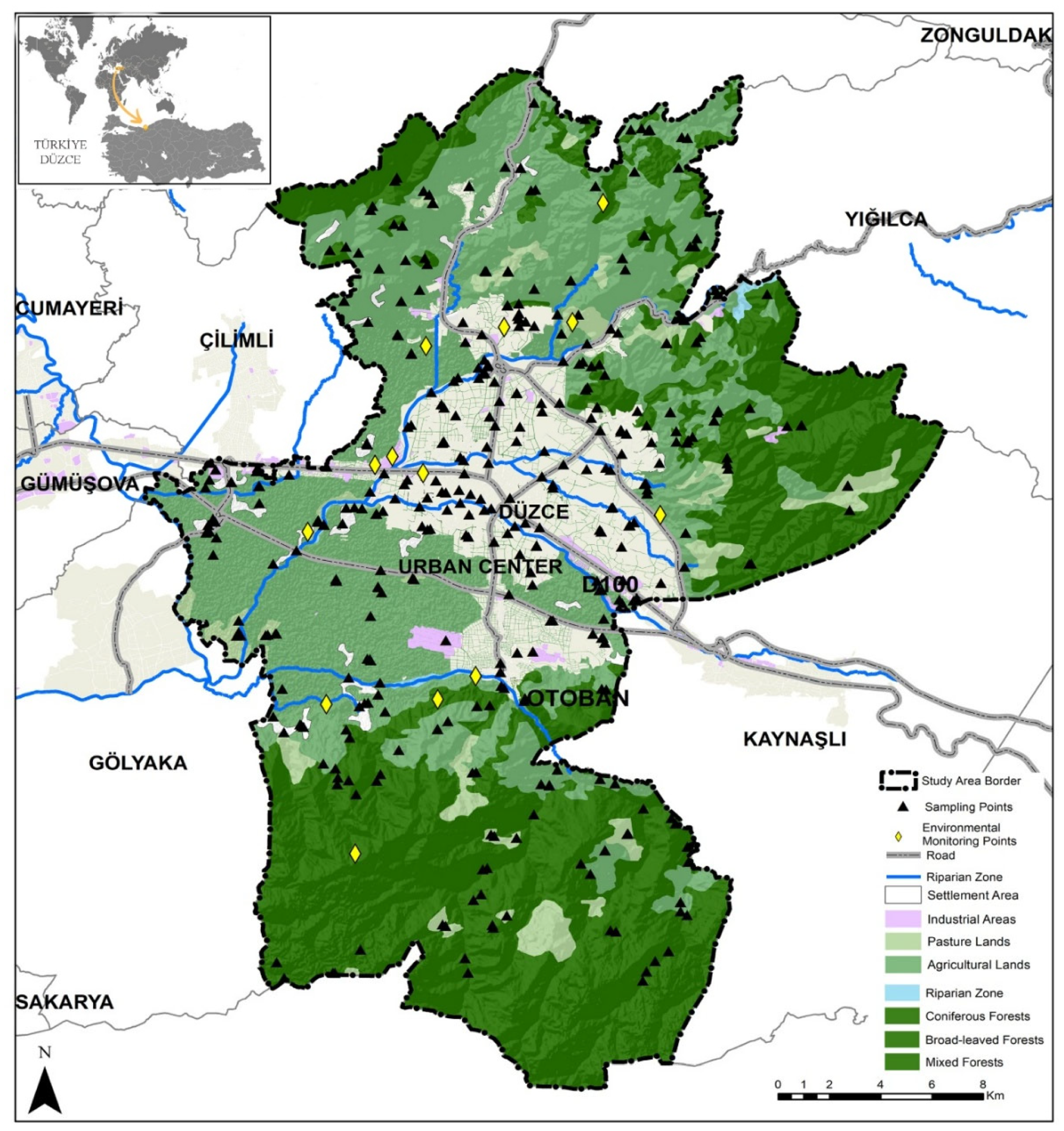
Figure 1. The spatial distribution of floristic sampling sites and environmental monitoring points overlaid on land cover classes and riparian corridors within the study area.
Diversity 17 00706 g001
Figure 2. Variations in Shannon Diversity Index (H′) Across Different CORINE Land Cover Groups (see Table 1 for group definitions). Each dot represents an individual sampling site, while blue diamonds and error bars indicate mean values and standard deviations for each CORINE land-cover group.
Diversity 17 00706 g002
Figure 3. Variations in Species Richness Across Different CORINE Land Cover Groups (see Table 1 for group definitions). Each dot represents an individual sampling site, while blue diamonds and error bars indicate mean values and standard deviations for each CORINE land-cover group.
Diversity 17 00706 g003
Figure 4. Variations in Pielou’s Evenness Index Across CORINE Land Cover Categories (see Table 1 for group definitions). Each dot represents an individual sampling site, while blue diamonds and error bars indicate mean values and standard deviations for each CORINE land-cover group.
Diversity 17 00706 g004
Figure 5. Top 10 most influential environmental predictors of plant species Diversity (Shannon_H) based on RF permutation importance analysis.
Diversity 17 00706 g005
Figure 6. Top 10 most influential environmental predictors of plant species Richness based on RF permutation importance analysis.
Diversity 17 00706 g006
Figure 7. Top 10 most influential environmental predictors of plant species Evenness based on RF permutation importance analysis.
Diversity 17 00706 g007
Figure 8. Observed vs. predicted values and residual distributions for Shannon Diversity, Species Richness, and Evenness based on RF regression models. (The left column shows the model fit between observed and predicted values for (a) Shannon Diversity Index, (c) Species Richness, and (e) Evenness, each accompanied by coefficient of determination (R2). The right column presents residual plots corresponding to each variable—(b,d,f)—demonstrating homoscedasticity and the absence of systematic bias across predicted values, supporting model reliability across urban ecological gradients). Blue dots represent observed vs. predicted values from Random Forest regression models, red lines indicate model fits, and shaded areas represent 95% confidence intervals.
Diversity 17 00706 g008
Figure 9. Observed vs. predicted values and residual distributions for Shannon Diversity, Species Richness, and Evenness based on native-only models. (a,b) Shannon Diversity Index predicted by XGBoost regression (R2 = 0.937474); (c,d) Species Richness predicted by Random Forest regression (R2 = 0.855305); and (e,f) Evenness predicted by Random Forest regression (R2 = 0.631796). (The left column shows the model fit between observed and predicted values for (a) Shannon Diversity Index, (c) Species Rich-ness, and (e) Evenness, each accompanied by coefficient of determination (R2). The right column presents residual plots corresponding to each variable—(b,d,f)—demonstrating homoscedasticity and the absence of systematic bias across predicted values, supporting model reliability across urban ecological gradients). Blue dots represent observed vs. predicted values from Random Forest regression models, red lines indicate model fits, and shaded areas represent 95% confidence intervals.
Diversity 17 00706 g009
Figure 10. Moran’s I test result for residuals of the RF model predicting Shannon diversity (H′).
Diversity 17 00706 g010
Figure 11. Model Generalizability Diagnostics: (a) 50-fold Hold-out R2 Distribution; (b) Y-shuffle Permutation Test.
Diversity 17 00706 g011
Table 1. Spatial Distribution of Sampling Sites According to Land Cover Categories.
Land Cover (Level 2)Land Cover (Level 3)SubtypeNo. of PlotsMinimum No. of Subplots
1.1. Urban Fabric1.1.1. Continuous Urban FabricPark/Urban Green Space291
1.1.2. Discontinuous Urban FabricResidential Area/Orchard/Annual Crops/Urban Void/Coppice29≥2
1.2. Industrial, Commercial, and Transport Units1.2.1. Industrial and Commercial UnitsIndustrial Site/University Campus91
1.2.2. Road and Rail Networks and Associated LandRoad Verge111
1.3. Mine, Dump, and Construction Sites1.3.1. Mineral Extraction SitesQuarry31
1.3.3. Construction SitesUrban Green Space11
2.1. Arable Land2.1.2. Permanently Irrigated LandCoppice/Annual Crops52
2.2. Permanent Crops2.2.2. Fruit Trees and Berry PlantationsOrchard181
2.3. Pastures2.3.1. Pasture LandPasture 91
2.4. Heterogeneous Agricultural Areas2.4.2. Complex Cultivation PatternsOrchard/Coppice/Annual Crops/Irrigated Crops/Ornamental Plants27≥2
2.4.3. Land Principally Occupied by Agriculture with Significant Areas of Natural VegetationAgricultural Use/Forest102
3.1. Forests3.1.1. Broad-leaved ForestsBroad-leaved Forest452
3.1.2. Coniferous ForestsConiferous Forest32
3.1.3. Mixed ForestsMixed Forest112
3.2. Maquis and Herbaceous Vegetation3.2.1. Natural GrasslandsNatural Grassland11
3.2.4. Transitional Woodland-ShrubForest/Shrubland21
4.1. Inland Wetlands4.1.1. Inland WetlandsInland Wetland2≥2
5.1. Inland Waters5.1.1. Water CoursesRiparian Zone151
Total 270397
Table 2. Abbreviations and Descriptions of Environmental Variables Used in the Analysis.
Variable DescriptionAbbreviation (Code)Variable DescriptionAbbreviation (Code)
Slope slopeMoisture at Wilting Point (%)Moisture_WP_%
Terrain Aspect Indexterrain_aspect_IndexTotal carbonate content in soil (%)% CaCO3_soil
Topographic Position IndextpiSoil moisture content (%)soil_moisture
Topographic RoughnessroughnessLight intensity measured in luxLight_Intensity
Terrain Ruggedness IndextriSoil temperature (°C)soil_temperature
ElevationelevationpH of precipitationpH_Rainwater
Aspect Suitability IndexBU_OAElectrical conductivity of precipitation (µS/cm)EC_Rainwater
Topography-based potential solar radiationHA_OACarbonate ion in precipitation CO3_Rainwater
Annual total solar radiationRA_OABicarbonate ion in precipitationHCO3_Rainwater
Mean annual solar radiationsolar_radChloride ion in precipitation Cl_Rainwater
Coarse fragment percentage in soilcoarse_frag_percentSulfate ion in precipitation SO42− in Rainwater
% Organic MatterOM_ percentCalcium ion in precipitation Ca2+ in Rainwater
Total Carbon (Organic + Inorganic)Total Carbon_%Potassium ion in precipitation K+ in Rainwater
Inorganic Carbon PercentInorganic Carbon_%Magnesium ion in precipitationMg2+ in Rainwater
Organic Carbon PercentOrganic Carbon_%Sodium ion in precipitationNa+ in Rainwater
Soil Electrical ConductivityEC_soilBioclimatic Variablesbio1, bio2… bio19
Soil pH (acidity–alkalinity)pH_soilDistance to riparian zones Riparian_Dist
Sand content in soil (%)sand_%Distance to forest areas Forest_Dist
Clay content in soil (%)Clay_%Distance to Urban Center Urban_Center_Dist
Silt content in soil (%)Silt_%Distance to roadsRoad_Dist
Moisture at Field Capacity (%)Moisture_FC_%Distance to industrial areasIndustry_Dist
Table 3. Feature Standardization and Multicollinearity Mitigation.
StepDescription Justification
(a) StandardScaler Each continuous variable was standardized using the z-score transformation formula x^ = (x − x¯)/s, such that the resulting values had an approximate mean of 0 and a standard deviation of 1.Ensures comparability among variables with different units by bringing them onto a common scale.
Reduces the influence of outliers compared to Min-Max normalization.
Enhances numerical stability in non-tree-based algorithms (e.g., SVR).
(b) High-Correlation Filter Absolute Pearson Correlation Coefficientρ
(c) VIF For the remaining columns, variables with VIF > 10 were iteratively removed.Multicollinearity inflates the variance of coefficient estimates; the VIF serves as its statistical diagnostic measure.
Table 4. Comparison of Algorithmic Performance Based on Model Characteristics and Test Set Accuracy.
AlgorithmStrengthsLimitationsR2 Score (Test Set)
RFAssumption-free; highly robust to outliersLimited interpretabilityHighest
XGBoostFast boosting; achieves high accuracy with fewer treesSensitive to hyperparameter tuning; prone to overfittingModerate
SVR (RBF Kernel)Suitable for small datasets with complex decision boundariesHighly sensitive to feature scaling; requires extended training timeLowest
Table 5. Model Cross-validation Results.
Shannon DiversitySpecies RichnessEvenness
CV R2 (10 × 5)0.968 ± 0.0140.948 ± 0.0220.858 ± 0.035
CV RMSE (10 × 5)0.047 ± 0.0104.427 ± 0.7330.021 ± 0.002
OOF R20.9700.9520.861
OOF RMSE0.0474.4080.021
Hold-out R2 (50×)0.966 ± 0.0120.942 ± 0.0160.846 ± 0.026
Hold-out RMSE (50×)0.049 ± 0.0074.731 ± 0.5880.022 ± 0.002
Y-shuffle R2−0.181−0.224−0.227
Disclaimer/Publisher’s Note: The statements, opinions and data contained in all publications are solely those of the individual author(s) and contributor(s) and not of MDPI and/or the editor(s). MDPI and/or the editor(s) disclaim responsibility for any injury to people or property resulting from any ideas, methods, instructions or products referred to in the content.