Article

An Invisible Boundary between Geographic Ranges of Cryptic Species of Narrow-Headed Voles (Stenocranius, Lasiopodomys, Cricetidae) in Transbaikalia

by
Tatyana V. Petrova
1,*,
Ivan A. Dvoyashov
1,
Yury A. Bazhenov
2,
Ekaterina V. Obolenskaya
1,3 and
Andrey A. Lissovsky
4,*
1
Laboratory of Evolutionary Genomics and Paleogenomics, Zoological Institute of Russian Academy of Sciences (RAS), Saint Petersburg 199034, Russia
2
Institute of Natural Resources, Ecology and Cryology, Siberian Branch of RAS, Chita 672014, Russia
3
Zoological Museum of Moscow State University, Moscow 125009, Russia
4
A.N. Severtsov Institute of Ecology and Evolution, RAS, Moscow 119071, Russia
*
Authors to whom correspondence should be addressed.
Diversity 2023, 15(3), 439; https://doi.org/10.3390/d15030439
Submission received: 30 December 2022 / Revised: 10 March 2023 / Accepted: 13 March 2023 / Published: 16 March 2023
(This article belongs to the Special Issue Phylogeny and Phylogeography of the Holarctic)

Abstract

:
The narrow-headed vole species complex is represented by Lasiopodomys gregalis and L. raddei, which probably diverged at the beginning of the Middle Pleistocene and came into secondary contact in the Transbaikal region. The current study analyzed mitochondrial gene cytochrome b, nuclear gene BRCA1, and microsatellite data and was aimed at clarifying geographic ranges of these species and searching for hybrid zones between them. It turned out that the geographic range of L. raddei is almost surrounded by that of L. gregalis; these species are strictly parapatric without a single detected sympatry zone. Although in none of the tested populations did the BRCA1 genotyping contradict the pattern revealed by mitochondrial cytb, microsatellite loci showed traces of hybridization in several populations. Results of species distribution modeling indicated that these species are characterized by quite similar (caused by the same environmental factors), but nevertheless significantly different, ecological preferences.

Graphical Abstract

1. Introduction

Competition theory [1] postulates that ecologically similar coexisting species are forced to partition resources and therefore one ecological niche cannot be inhabited by multiple species because fitter ones should eventually displace the rest [2,3]. It is expected that closely related species that are similar morphologically, physiologically, and behaviorally will also be ecologically alike and will show little niche differentiation [4,5], but some studies indicate that cryptic species are less likely to co-occur than related but noncryptic ones [6].
Secondary contact zones are of particular interest for evolutionary biologists because of unique opportunities to assess the level of reproductive isolation between closely related taxa that differentiated recently [7]. If strong reproductive barriers have already formed under the conditions of allopatry, then during the transition to secondary contact, the groups will not be able to mix their genomes. On the contrary, if reproductive isolation has not been reached, then as a result of hybridization, the genetic divergence that has developed allopatrically is erased, and eventually, a complete merging of the parental genomes occurs [8]. Between recently diverged young taxa, hybridization takes place often. Nonetheless, due to the presence of prezygotic and postzygotic reproductive barriers, the gene flow between the groups weakens [9].
Narrow-headed voles of the subgenus Stenocranius (Lasiopodomys, Cricetidae) are a widespread group of rodents known to exist since the Pleistocene when Stenocranius was a characteristic component of mammoth fauna [10,11,12]. Its geographic range was continuous, occupied the territory of the tundra-steppe, and extended almost to the entire territory of the northern Palearctic. With the formation of a wide taiga zone in the Holocene, its geographic range broke up into several isolated regions. Currently, narrow-headed voles inhabit various open landscapes: from tundra and local sandy areas along major rivers to alpine meadows and steppes [13].
It has been shown that the narrow-headed vole species complex is represented by at least two species, which probably diverged at the beginning of the Middle Pleistocene (~0.8 Mya) [14]: Lasiopodomys gregalis Pallas, 1779, which is widespread throughout the Palearctic, and L. raddei Poljakov, 1881, which occurs in patches within southeastern Transbaikalia. Lasiopodomys gregalis is represented by three strongly diverged genetic lineages: A, B, and C [14]. Lineage A was involved in wide Pleistocene migrations mentioned above. Lineage C is endemic to southeastern Tuva. The third one, lineage B, occurs in arid areas across Mongolia from Lake Ubsunur in the west to the northern Transbaikalia and Amur Region. This lineage is the subject of the current study, and therefore all L. gregalis populations mentioned below are voles of lineage B.
Lasiopodomys raddei is indistinguishable from L. gregalis after craniological analysis [15]. Moreover, these taxa are so similar in morphology that L. raddei and L. gregalis lineage B have been combined into one subspecies—L. gregalis raddei Poljakov, 1881—for a long time, until molecular methods were applied. Furthermore, the type series of the nominal taxon raddei Poljakov, 1881, includes specimens of both species [16]. Lasiopodomys raddei was elevated to the status of a full-rank cryptic species after an analysis of nuclear genes, of experimental hybridization, and of the morphology of first lower (m1) and third upper (M3) molars [16].
In previous studies [14,15,16], we hypothesized that the northwestern limit of the L. raddei geographic range lies along the forested northern bank of the Shilka and Ingoda rivers. The southern border is still unknown. We did not find any localities where the two species co-occur after an analysis of mitochondrial cytochrome b (mt cytb) and nuclear breast cancer 1 gene (BRCA1) exon 11 in several individuals from the border territory [16]. We did not detect any signs of nuclear–mitochondrial discordance between the species, either.
The first purpose of this study was to clarify spatial relationships between the two cryptic species. We performed ecological niche modeling to evaluate differences in ecological preferences between the species. The second purpose was to understand whether there is a gene flow between the taxa or if they are reproductively isolated.

2. Materials and Methods

2.1. Sampling and DNA Isolation

In total, 178 narrow-headed voles from 57 localities in the Transbaikal region and Eastern Mongolia were included in the molecular analysis; eight museum specimens collected between years 1935 and 1985 were genotyped too (see Figure 1 and Table S1 for details). The study was conducted according to the guidelines of the Declaration of Helsinki, and the study protocol was approved by the Ethics Committee at the Zoological Institute of the Russian Academy of Sciences (RAS; St. Petersburg) (permission #3-17, 14 November 2022).
Isolation of genomic DNA from fresh muscle tissue samples stored in 96% ethanol was performed using the ExtractDNA Blood & Cells Kit (Evrogen, Moscow, Russia). DNA from museum skin samples was isolated with the QIAmp Tissue Kit (Qiagen, Hilden, Germany). To reduce potential contamination, all manipulations with the museum specimens were carried out in a separate laboratory room isolated from post-PCR facilities predominantly being used for studies on historic samples from the collection at the Zoological Institute of RAS. All the working surfaces, instruments, and plastics were sterilized with UV light and chloramine-T.

2.2. Amplification of Mitochondrial Cytb and Nuclear BRCA1

A part of the cytb gene was amplified with primers UCBU and LM by a standard protocol described elsewhere [17].
To check mtDNA for introgression between the species, we amplified BRCA1 from DNA of some specimens from the border zone between the species’ geographic ranges. The BRCA1 nuclear marker has previously shown a high degree of interspecific variation [16]. Several old museum specimens were genotyped by means of BRCA1 fragments (Table S1, Sheet 2) as well. BRCA1 was amplified using primers F180_arv and R1240_arv via the PCR protocol published by Bannikova et al. [18]. To amplify short fragments from dry museum skin samples, two pairs of primers were designed: BRCA_F224 5′-GCA CAT CTG ACA GGA GGC ACG GC-3′/BRCA_R357 5′-GAA AGC TCT GTG GGG ATC AGA GGC C-3′ and BRCA_F586 5′-GCA GAT TTA ACA GTT ACT CAA AAG AC-3′/BRCA_R719 5′-GTA TGA AGA TTA TTA CCT TTT GCT CCG-3′. Each target fragment (83 and 81 bp, respectively) contains three specific SNPs that distinguish one species from the other. The thermal cycling program consisted of an initial 10 min denaturation step at 95 °C, followed by 40 cycles of 30 s at 94 °C, 30 s at 60 °C (F224/R357) or 52 °C (F586/R719), 30 s at 72 °C, and a final 7 min elongation step at 72 °C. PCR mixtures were prepared using a PCR workstation (LAMSYSTEMS CC, Miass, Russia).
Sequences obtained in the current study were deposited in GenBank under the following accession numbers: OP765403–OP765443 and OP765446–OP765490 (cytb) and OP781557–OP781588 and OQ201578–OQ201592 (BRCA1). Sequences of short BRCA1 fragments amplified from the DNA of museum specimens (these sequences could not be uploaded to GenBank due to their short length) are given in Supplementary Materials (File S1). For detailed information on the analyzed specimens, sampling localities, GenBank accession numbers, and other data, see Table S1.

2.3. Amplification of Microsatellite Loci

We chose six microsatellite loci described for L. gregalis: Mar049, Mar076, Mar080, MSMM2, MSMM6, and MSMoe02 [19]. Forward primers were labeled with a fluorescent dye—FAM, R6G, or TAMRA (Syntol, Moscow, Russia)—to enable separation of the resulting products; markers were multiplexed in two sets as described by Petrova et al. [20]. Capillary electrophoresis of the PCR products was implemented on an ABI Prism 3500xL Genetic Analyzer (Applied Biosystems Inc., Foster City, CA, USA) at Evrogen (Moscow, Russia).

2.4. Cytb Phylogenetic Reconstruction and BRCA1 Genotyping

Sequences were edited and aligned with the CLUSTALW algorithm [21] implemented in BioEdit [22]. Phylogenetic reconstruction based on cytb sequences was performed on 200 narrow-headed voles’ haplotypes with two specimens as an outgroup (Lasiopodomys mandarinus FJ986322 and L. brandtii JF906120). The final alignment comprised a 1018 bp cytb fragment. Bayesian inference analysis was carried out in MrBayes 3.2.6 [23] with the following parameters: nst = mixed, the distribution of substitution rates between sites, and the dataset was divided into partitions by codon position. Each analysis was started with a random tree and had two replicates with four Markov chains (MCMC) and 2 million generations, with the results recorded every 1000th generation. Stationarity and convergence of separate runs were assessed using ESS statistics in Tracer v1.7 [24]. A 50% majority rule consensus tree constructed based on trees sampled after a 25% burn-in was visualized by means of the FigTree v1.6 program (http://tree.bio.ed.ac.uk/software/figtree/, accessed on 26 November 2021).
Nuclear BRCA1 sequences were not used for phylogenetic reconstruction because the variation within each species was very low. We identified species by means of BRCA1 data while checking stable substitutions in the alignment (File S1).

2.5. Microsatellite Loci Analyses

2.5.1. Quality Control and Grouping of Samples

We amplified six microsatellite loci (see Section 2.3) in 143 specimens from 29 localities, but after the initial analysis, the MSMM6 locus was excluded due to multiple additional bands in capillary electrophoresis. The final analysis included only five loci (Mar049, Mar076, Mar080, MSMM2, and MSMoe02) for 119 specimens from 25 localities (Table S1).
We combined several neighboring populations into subgroups: sites 4 and 5 (Kharalga), sites 17 and 18 (vicinities of Kuytun), sites 22 and 23 (vicinities of Baley), and sites 47 and 49 (vicinities of Choibalsan); see Figure 1 and Table S1 for details.

2.5.2. Genetic Diversity Analyses

Observed (Ho) and expected (He) heterozygosity and the number of observed alleles (Na) per locus were calculated using Adegenet package v2.1.8 [25] as implemented in R software v4.2.1 [26] within the RStudio environment [27].
The frequency of a null allele (fna) per locus was calculated in PopGenReport [28]. Estimates of null allele frequency were obtained with both the method of Chakraborty et al. [29] and the method of Brookfield [30].
To correctly evaluate statistics per population, the populations with the number of specimens lower than five were excluded. FIS [31] for each remaining population and FST and Dst by Jost [32] among these populations were calculated using HIERFSTAT [33]. The number of private alleles (Np) and allelic richness (Ar) per population were calculated with the help of PopGenReport v3.0.4 [28]. Pairwise FST values across all populations were calculated in HIERFSTAT (Fst2x2 function), and significance was tested with 1000 bootstraps and a 95% confidence level. Deviations from the Hardy–Weinberg equilibrium were estimated for each locus at each sampling locality by means of Pegas package v1.1 [34], and the p-value was determined by Fisher’s method.

2.5.3. Population Structure Analysis

On the basis of the microsatellite data, principal component analysis (PCA) was performed by the methods implemented in R package Adegenet v2.1.8 (the dudi.pca function).
Underlying genetic structure in the studied populations was further investigated via a Bayesian clustering approach as implemented in STRUCTURE v2.3.4 [35]. The most likely number of clusters (K) was inferred using a simulation series with K ranging from 1 to 7, with 10 iterations for each K value. Each run was 300,000 generations in length with a burn-in of 100,000 generations. Optimal K was evaluated using STRUCTURE HARVESTER [36].

2.6. Species Distribution Modeling

2.6.1. Environmental Data

The spatial frame of the analysis included a grid with 2 km resolution in the geographic Mollweide projection. We utilized 62 variables in the main analysis: CHELSA 19 “bioclimatic” variables (https://chelsa-climate.org/downloads/ (accessed on 30 March 2021); Karger et al. [37]), altitude, and 42 MODIS generalized average monthly data layers (6 months of 2004 per seven spectral bands; http://glcf.umiacs.umd.edu/data (accessed on 15 October 2010), Eastern Hemisphere only) as environmental data. We used two spatial extents for the analyses. The first included the proposed whole range of L. raddei as well as the whole range of neighboring lineage B of L. gregalis from Transbaikalia and Eastern Mongolia. The second was the geographic range of L. gregalis excluding northern populations (tundra and intrazonal steppes).

2.6.2. Occurrence Data and Target Group Backgrounds

We employed information from museum specimens stored in collections of the Zoological Institute of RAS (St. Petersburg), the Zoological Museum of Moscow State University (Moscow), the Zoological Institute tissue collection, and data from research articles. To assign a locality to either L. gregalis or L. raddei, we relied on our genetic data and included all the sites from an area outlined by “genetic” sites as well. Only localities with precision of georeference of 2 km or less were included in the analysis. The initial dataset for the whole southern part of the combined geographic range included 605 records of L. gregalis and 101 of L raddei. The localities formed notable spatial aggregates. To reduce the effect of the aggregates on the analysis results, initially, we selected one occurrence point per 50 × 50 km square and then increased the side of the square by 3 km until Moran I was <0.25. Test sets were generated by similar filtering of the whole dataset but with the square side taken from the previous step and multiplied by 1.1. The final dataset of occurrences included 48 records of L. gregalis and 29 of L. raddei for the Transbaikal extent and 108 records of L. gregalis for the second spatial extent (Table S2, Figure S2). The numbers of specimens in the test sets were 47, 27, and 112, respectively.
To correct sampling bias, we applied the target group background approach [38]. Data on ecologically similar species with similar approaches to detection (all vole species and Striped-back Hamster Cricetulus barabensis Pallas, 1773) were retrieved from the same sources as described above. The total target group consisted of 4040 specimens.

2.6.3. Modeling

Species distribution modeling (SDM) was carried out in R [26] using a custom-designed script based on ENMeval [39,40] and maxnet [41,42] packages in MaxEnt v3.4.1 [41]. The underlying principle of the calculations was to select the best model on the basis of the corrected Akaike’s information criterion (AICc) values evaluated on the test sets from a series of models with different values of the regularization multiplier (0.75, 1, or 2), different sets of feature types (“L”, “LQ”, or “LQH”; where L = linear, Q = quadratic, and H = hinge) [39], and different sets of background points (BPs). Selection of BPs was crucial for these analyses. We constructed a surface with probability values for the BP selection. The values were computed as a decimal logarithm of the number of specimens of a target group species detected in every raster cell plus 0.1 multiplied by the number of specimens registered in every raster cell minus the evaluation of general sampling effort. The probability of BP selection within a “distribution range” (an area including 40 km buffers around occurrence points) was decreased by twofold.
The difference between two resulting models was calculated in both E- and G-space [43]. We compared two models (maps) in the case of G-space and compared rasterized scatterplots of the first two principal components of values of environmental parameters in occurrence points in the case of E-space. Schoener’s D was used for comparison [44,45]. The sample of occurrence points was randomized 100 times, preserving sample size and all model parameters for both “species”. The p-values were calculated by comparing Schoener’s D after an interspecies comparison with the distribution of simulated D values.
Because the result of the MaxEnt algorithm is relative habitat suitability, we chose a nonrigorous way to display distributions in figures. We used two ranges of habitat suitability values to draw spatial structure of a species distribution. The “optimal” core was drawn in a range of 0.75–1.00, and a “suboptimal” area in a range from maximum training sensitivity plus a specificity threshold to 0.75.

3. Results

3.1. Species Identification by Means of Cytb and BRCA1

The results of phylogenetic analysis of cytb (Figure 2) were consistent with a previous study [16] in terms of positions of the major clades of Stenocranius.
In addition to mt cytb, the BRCA1 nuclear gene was amplified for a number of populations (Table S1) to check for nuclear–mtDNA discordance. The results indicated that specimen identification by BRCA1 was completely consistent with the identification by cytb.
The old museum specimens were genotyped using only BRCA1. We were able to isolate DNA from eight of ten museum specimens initially planned for the analysis. The first gene fragment was successfully obtained from all the eight specimens, whereas the second one only from three of them, including the oldest specimen, collected in 1935 (Table S1, Sheet 2).

3.2. Population Structure Revealed by the Microsatellite Loci Analysis

3.2.1. Genetic Diversity Analysis

The five loci comprised 99 alleles (Table 1). The number of alleles per locus ranged between 18 (Mar076) and 22 (MSMM2), with an average of 19.8. Expected heterozygosity ranged between 0.880 (MSMoe02) and 0.927 (MSMM2), while observed heterozygosity ranged between 0.582 (Mar049) and 0.817 (Mar076). The average frequency of null alleles across all five loci, as inferred with the method of Chakraborty et al. [29], was 10%, whereas the value inferred with the Brookfield method [30], which takes into account the presence of null homozygotes, was 9.4% (Table 1).

3.2.2. Population Diversity Analysis
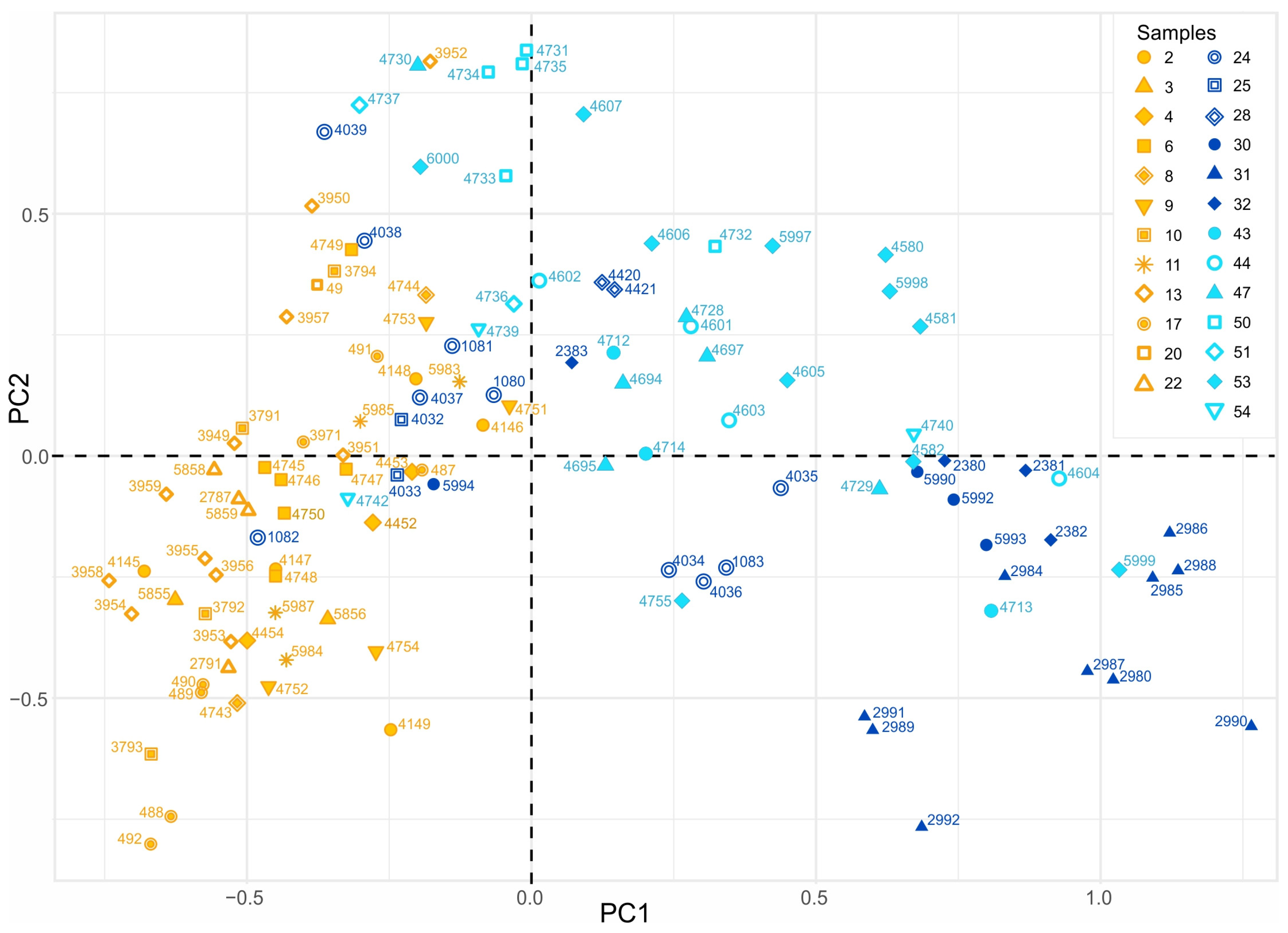
The mean allelic richness ranged between 2.9 and 4.2 among the nine sampling sites, with the lowest values detected in populations Indola (31) and Khavirga (50), and the largest values found in populations Elon-Obot (6) and Matakan (24) (Table 2). The average observed heterozygosity across five microsatellite loci was a bit higher than expected. The number of private alleles was the largest in populations Uldza, Kuytun, and Matakan (four, four, and seven private alleles, respectively). The inbreeding coefficient varied between −0.205 (Khavirga) and 0.188 (Matakan) (Table 2).
Pairwise FST estimates among populations (Table 3) indicated that the Indola site (locality ID 31) was the most distant one (FST = 0.151 to 0.312).

3.2.3. PCA

The PCA of allele frequencies of five microsatellite loci (Figure 3) did not show clear separation into clusters; nevertheless, each species occupies a distinct position in the cloud of points. Several populations of L. gregalis from the territory bordering with L. raddei (Figure 1, localities No. 24, 25, and 28) occupy an intermediate position between the two species clouds.

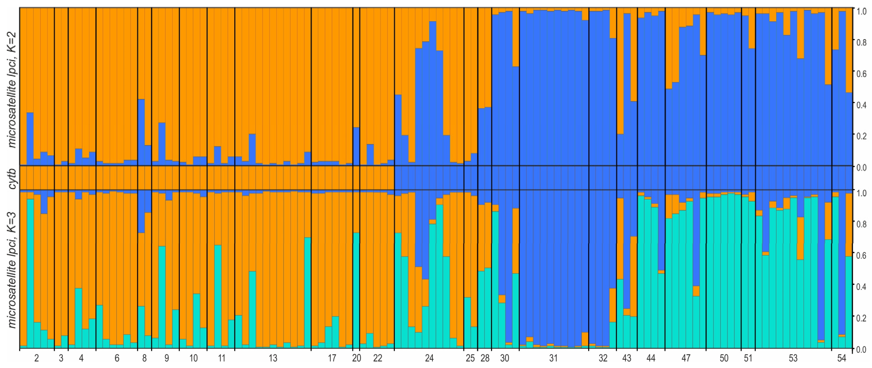
3.2.4. Population Structure

We identified two distinct clusters using STRUCTURE HARVESTER, with results similar between log-likelihood and Evanno approaches (Figure S2). These two clusters (Figure 4, upper row) roughly matched our results on mt cytb. Nevertheless, several localities (Figure 1; e.g., localities No. 24, 28, and 43) included individuals that could not be assigned to a specific cluster with Q values higher than 0.6 (Figure 4), while specimens from population 25 turned out to be L. gregalis according to the cytb analysis and “raddei-like” according to the microsatellite results. When divided into three clusters (Figure 4, lower row), a group from Buryatia (“pure gregalis”), a group from Eastern Mongolia, and L. raddei with an admixture of alleles from Eastern Mongolia could be distinguished.

3.3. Species Distribution Prediction

The best model for L. gregalis in Transbaikalia had a regularization multiplier of 1.0, the L (linear) feature type, and a 3.5 km buffer for BP selection. The best model for L. raddei had a regularization multiplier of 2.0, the L (linear) feature type, and a 5 km buffer for BP selection. The list of factors influencing the distribution was similar between the two species. In the case of L. raddei, the biggest permutation importance belonged to maximal depth of snow (42.54), followed by the first (23.69) and the sixth (22.32) bands of the September MODIS shot. In L. gregalis, the biggest permutation importance belonged to the fourth band (41.03) of the September MODIS shot, followed by precipitation in the wettest month by CHELSA (16.02). Nevertheless, the first (13.66) band of the September MODIS shot and the maximal depth of snow (5.35) also had big importance. Voles were found to differ in the tolerance range of these two variables. Lasiopodomys gregalis is more tolerant of deeper snow, whereas L. raddei inhabits a wider range of MODIS band values (Figure S3).
The model of the southern part of the L. gregalis geographic range had a regularization multiplier of 1.0, LQ (linear + quadratic) feature types, and a 5 km buffer for BP selection. The set of factors (minimal temperature of the coldest month (21.47) and precipitation in the wettest quarter (16.60)) was expectedly different from that of the Transbaikal model, which takes into account a different spatial scale [46].
In the Transbaikal extent, the distributions of suitable habitats notably differed between L. gregalis and L. raddei (Figure 5). The structure of the spatial distribution of suitable habitats in each species has a characteristic feature. Each species has a zone of continuous suitable habitats and a wider territory where suitable habitats have a mosaic distribution. In the case of L. raddei, the continuous “core” zone includes a territory between the Aga and Argun Rivers, toward the south to ~49° N. Large isolated patches of suitable habitats are situated in the middle reaches of the Ingoda River and west of this area, in upper reaches of the Onon River, and in the middle Selenga River. Another big suitable area lies east and south of Lake Dalai-Nur, although it is separated from the main “core” by a narrow belt of unsuitable territory. In the case of L. gregalis, the continuous “core” zone is found south of the Torey Lakes and south and east of Lake Dalai-Nur. The rest of the territory has a rather mosaic pattern of suitable habitats. Thus, the overlap between the “core” zones of the two species includes a small territory south of the Torey Lakes and to the south and east of Lake Dalai-Nur. There is another predicted area, on the right bank of the Argun River and on the northern shore of Lake Dalai-Nur, where we have no data.
The models for L. gregalis and L. raddei in Transbaikalia significantly differed both in geographic space (Schoener’s D: 0.66, p-value: 5.15 × 10⁻⁸) and environmental space (Schoener’s D: 0.28, p-value: 0.009). The model of the southern part of the L. gregalis range differed from the Transbaikal model for the same species in the pattern of distribution of suitable habitats. In the first case, the distribution of habitats of L. raddei was found to be suitable for L. gregalis.
The majority of the populations studied by microsatellite loci analysis falls into habitats suitable for the respective species. Nearly all specimens that possess microsatellite alleles similar to those of L. raddei were collected in places suitable for this species, except for specimens No. 3, 31, and 43. Specimens 31 and 43 from this list were collected far from the L. raddei range. The only specimens that bear alleles similar to those of L. gregalis but were collected in places with low suitability for L. gregalis are No. 3, 6, 9, 10, and 20. All of them were collected within the L. raddei geographic range and far from the L. gregalis range.

4. Discussion

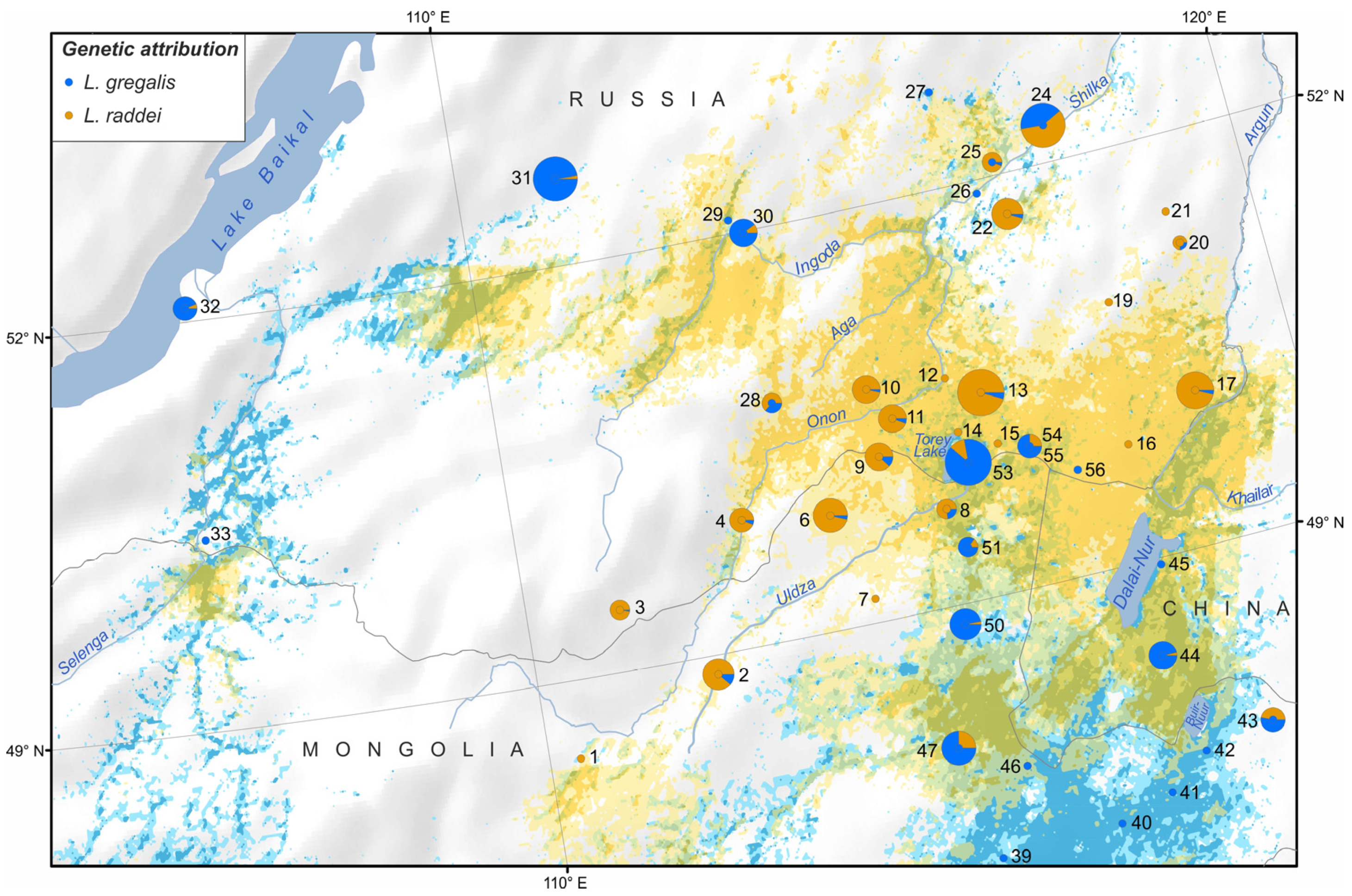
4.1. Clarification of Cryptic Species’ Ranges

Our new genetic data made it possible to clarify the distribution of two cryptic species of narrow-headed voles. The results of this study showed that Eastern Mongolia and the adjacent Inner Mongolia province of China are inhabited by representatives of L. gregalis (Figure 1). For instance, the geographic range of L. raddei is almost surrounded by that of L. gregalis. At the same time, we did not find any case of a sympatric distribution of these species, even in the area of “core” habitats’ overlap. A similar distribution map was published by Kryshtufek and Shenbrot [47], probably on the basis of our older limited dataset because we are now publishing detailed data on the L. raddei range for the first time.
The results of microsatellite analysis imply a gene exchange across a big territory. The biggest inconsistency between species identification based on individual genes and microsatellite results was noted at the western limit (Figure 5, locality No. 28) and northern limit (Figure 5, localities No. 24 and 25) of the L. raddei range. These localities correspond to a zone of mosaic distribution of habitats suitable for the two species. The problem with the northern limit of the L. raddei range—which, as we hypothesized previously, could be easily explained by the forested northern bank of the Shilka and Ingoda rivers [14,15,16]—turned out to be more complicated. Our results on genotyping by means of one mitochondrial and one nuclear gene assigned voles from the left bank of the Shilka River to L. gregalis again, while microsatellite results suggested the prevalence of L. raddei alleles there.
In addition, we found a bigger microsatellite polymorphism in the overlap between “core” suitable habitats of the two species (Figure 5, localities No. 8, 53, and 54). A similar pattern was also documented in areas where one of the species has not been found yet, but suitable habitats for both species are present (Figure 5, localities No. 29 and 47). Some “alien” alleles were found in other localities, too. The general pattern of genetic variation more resembles a temporal fluctuation of the geographic ranges of the two species rather than existence of any strong barriers between them. We can theorize that the border regions that are covered with scattered habitats suitable for both species as well as the zone of “core” habitats’ overlap are sometimes inhabited by one or the other species. The outcome may depend on population dynamics and distance to the nearest stable population [48]. As a consequence of this temporal pattern, we observe higher microsatellite polymorphism in the regions discussed above but cannot find any signs of species sympatry. We are aware of all the limitations imposed by the small number of analyzed microsatellite loci. Probably, a wider panel of microsatellite loci SNP data will help to elucidate this complex study case.
A less problematic area is a southwestern limit of the L. raddei range (Figure 1, localities No. 1–3). According to SDM results, forested northern Khentii represents a strong geographic barrier between L. raddei and populations of L. gregalis from the Selenga River basin. An eastern limit of the L. raddei range is still unknown. Our genetic data can trace the L. raddei range as far to the east as the left bank of the Argun River (Figure 1, localities No. 16–21). According to our modeling results, there is an overlap between “core” suitable habitats of the two species on the right bank of the Argun River. This zone of the overlap extends south to the eastern shore of Lake Dalai-Nur as well. Unfortunately, we have no data from this region and cannot check the genetic variation there.
Our study cannot shed light on the problem of the taxonomic position of described nominal taxa from the region under consideration. Because the nominal taxon raddei Poljakov, 1881, is the oldest taxon in the group, the name of this species is stable. The name of L. gregalis lineage B, if one has to assign taxonomic status to it, remains unclear. There are two described nominal taxa of Stenocranius from this region: Stenocranius angustus Thomas, 1908, and Microtus g. sirtalaensis Ma, 1965. The type series of both taxa are still unavailable for us.
The nominal taxon Stenocranius angustus Thomas, 1908 was described from the territory of Northeastern China (100 miles NW from Kalgan). Specimens from the L. g. angustus type locality were not analyzed by us due to the lack of the biological material; however, morphological characteristics of the type specimen (simplified upper M3 and light fur color) published by Thomas [49] clearly match the diagnostic features of L. raddei [50]. Therefore, there may be one more isolate of L. raddei in Northeastern China. The type series of L. g. sirtalaensis from Sirtala, Inner Mongolia, was not available for our molecular analysis. Nonetheless, if we assume the existence of differences in the species’ fur color, then dark L. g. sirtalaensis [51] more likely represents L. gregalis than more lightly colored L. raddei.
Kryshtufek and Shenbrot [47] assigned nominal taxa L. g. sirtalaensis and L. g. angustus to L. gregalis, although the grounds for this taxonomic decision are unclear.

4.2. Searching for Isolation Mechanisms

Our previous study [16] shows that representatives of L. gregalis lineage B (albeit captured not in the Transbaikal Region but in the western part of the L. gregalis lineage B geographic range) produce offspring in pairs with L. raddei. Nonetheless, in that study, the success of reproduction varied among reciprocal combinations. Unfortunately, we were unable to test the fertility of F1 males.
Judging by the findings of the current study, a gene flow takes place between these cryptic species, but it is unclear how it proceeds because no sympatry sites were found. The only possible explanation we see is that the dispersal of species into an isolated territory occurs during population peaks, consistent with the report of Waters et al. [52]. Thus, the “border” between the two species may be unstable. Meanwhile, several factors are definitely important in this regard, such as the distance from an isolate to the main range of the species and the presence of surmountable geographical barriers (e.g., rivers and local taiga areas) which, albeit slightly, reduce the gene flow, thereby allowing a population to form (that is genetically isolated to some extent) on the sides of the “barrier”.
It is impossible to rule out the presence of some behavioral mechanisms that limit the gene flow. For instance, a Gene Ontology enrichment analysis of RNA-Seq data from both species [53] has identified approximately a hundred biological processes associated with genes having contrasting SNPs. Among them, processes of interspecific interactions, defense responses, responses to external stimuli, and the perception of chemical stimuli and smell were found, indicating the likely existence of precopulatory behavioral and physiological mechanisms that contribute to the isolation between these cryptic species. An analysis of selective pressure in individual orthologs has also yielded a list of genes that may be involved in reproductive processes and ecological adaptations.
Vocal communication may also play some role in the behavioral isolation. As shown by Rutovskaya and Nikolsky [54], the narrow-headed vole, as an animal with well-developed sociality, has a vocal repertoire that has developed the best among voles and is comparable to that of social Brandt’s vole Lasiopodomys brandtii Radde, 1861 [55]. All four types of sound signals—an alarm signal, sharp squeaks (characteristic of animals fighting among themselves), quiet squeaks (recorded during friendly contacts between animals, courtship, or soft avoidance of contact), and songs of males during courtship—proved to vary widely among populations in that report. Nonetheless, those authors did not compare these signals between L. raddei and neighboring populations of L. gregalis; this is the subject for further research.

5. Conclusions

Our analysis of new data from a border zone between geographic ranges of cryptic species L. gregalis and L. raddei revealed that the geographic range of L. raddei is almost surrounded by L. gregalis’s one. These species are strictly parapatric without a single detected sympatric case, and this pattern would be expected if these species were reproductively isolated completely. Although microsatellite loci show traces of hybridization in several populations, BRCA1 genotyping did not detect introgressions of the mt genome, thereby fully conforming to the pattern manifested by mt cytb.
Results of species distribution modeling indicate that the two species are characterized by similar (caused by the same environmental factors: maximal depth of snow and precipitation in the wettest month), but nevertheless significantly different, ecological preferences.
It is still unclear which mechanisms contribute to the population differentiation of these species along the entire parapatric zone except for the northwestern limit of the L. raddei geographic range, where the differentiation is explained by a barrier along the Shilka River. Dispersion of one of the cryptic species into isolated territories may occur during asynchronous population peaks; consequently, the “border” between the two species may be unstable. Perhaps some behavioral features and interactions between these rodents are important in this regard.

Supplementary Materials

The following supporting information can be downloaded at https://www.mdpi.com/article/10.3390/d15030439/s1, Figure S1: Occurrence records used for species distribution modeling of Lasiopodomys gregalis and L. raddei; Figure S2: Detecting the number of clusters of individuals; Figure S3: Suitable ranges of shared factors’ values for L. gregalis and L. raddei; Figure S4: The scheme of the proposed distribution of Lasiopodomys gregalis and L. raddei and localities used for SDM; Table S1: The material used in the genetic analyses; Table S2: Occurrence records employed for species distribution modeling; File S1: BRCA1 alignment including short sequences from museum specimens.

Author Contributions

Conceptualization, T.V.P. and A.A.L.; methodology, T.V.P., I.A.D. and A.A.L.; formal analysis, T.V.P., I.A.D. and A.A.L.; investigation, T.V.P., I.A.D., Y.A.B., E.V.O. and A.A.L.; data curation, T.V.P. and A.A.L.; writing—original draft preparation, T.V.P., I.A.D., Y.A.B., E.V.O. and A.A.L.; writing—review and editing, T.V.P., I.A.D., Y.A.B., E.V.O. and A.A.L.; visualization, T.V.P., I.A.D., E.V.O. and A.A.L.; supervision, T.V.P.; funding acquisition, T.V.P. All authors have read and agreed to the published version of the manuscript.

Funding

This research was funded by the Russian Science Foundation (RSF), grant No. 22-24-00513 (https://rscf.ru/project/22-24-00513/).

Institutional Review Board Statement

The study was conducted according to the guidelines of the Declaration of Helsinki, and the study protocol was approved by the Ethics Committee at the Zoological Institute of the RAS (permission # 3-17, 14 November 2022).

Data Availability Statement

Sequences obtained in the current study were deposited in GenBank under the following accession numbers: OP765403–OP765443 and OP765446–OP765490 (cytb) and OP781557–OP781588 and OQ201578–OQ201592 (BRCA1); see Table S1 for details. Occurrence points of L. gregalis and L. raddei from the Russian part of Transbaikalia were submitted to the Mammals of Russia database: https://rusmam.ru/sample/records?id=s_2_d62e7a0b82 (accessed on 27 October 2022). Other raw data are available upon request.

Acknowledgments

We express our gratitude to N.I. Abramson (Zoological Institute of RAS), under whose leadership this project began. We are grateful to L.L. Voyta (Zoological Institute of RAS), B.I. Sheftel (A.N. Severtsov Institute of Ecology and Evolution RAS), R. Samiya (National University of Mongolia), Liu Songtao and Dou Huashan (Hulun Lake Nature Reserve, Inner Mongolia, China) for help with collecting the material and for providing tissue samples, and to V.S. Lebedev (Zoological Museum, Moscow State University), who allowed us to analyze tissue samples from the museum collection. We thank P.A. Sorokin (A.N. Severtsov Institute of Ecology and Evolution, RAS) for help with the analysis of microsatellite loci, and three anonymous reviewers for their helpful and critical comments. The English language was corrected by shevchuk-editing.com.

Conflicts of Interest

The authors declare no conflict of interest.

References

  1. Hardin, G. The Competitive Exclusion Principle: An Idea That Took a Century to Be Born Has Implications in Ecology, Economics, and Genetics. Science 1960, 131, 1292–1297. [Google Scholar] [CrossRef] [PubMed] [Green Version]
  2. Gause, G.F. Experimental Studies on the Struggle for Existence. J. Exp. Biol. 1932, 9, 389–402. [Google Scholar] [CrossRef]
  3. Holt, R.D.; Grover, J.; Tilman, D. Simple Rules for Interspecific Dominance in Systems. Am. Nat. 1994, 144, 741–771. [Google Scholar] [CrossRef]
  4. Violle, C.; Nemergut, D.R.; Pu, Z.; Jiang, L. Phylogenetic Limiting Similarity and Competitive Exclusion: Phylogenetic Relatedness and Competition. Ecol. Lett. 2011, 14, 782–787. [Google Scholar] [CrossRef] [PubMed]
  5. Cothran, R.D.; Henderson, K.A.; Schmidenberg, D.; Relyea, R.A. Phenotypically Similar but Ecologically Distinct: Differences in Competitive Ability and Predation Risk among Amphipods. Oikos 2013, 122, 1429–1440. [Google Scholar] [CrossRef]
  6. Vodă, R.; Dapporto, L.; Dincă, V.; Vila, R. Why Do Cryptic Species Tend Not to Co-Occur? A Case Study on Two Cryptic Pairs of Butterflies. PLoS ONE 2015, 10, e0117802. [Google Scholar] [CrossRef] [Green Version]
  7. Barton, N.H.; Hewitt, G.M. Analysis of Hybrid Zones. Annu. Rev. Ecol. Syst. 1985, 16, 113–148. [Google Scholar] [CrossRef]
  8. Endler, J.A. Geographic Variation, Speciation, and Clines; Princeton University Press: Princeton, NJ, USA, 1977. [Google Scholar]
  9. Hewitt, G.M. Hybrid Zones-Natural Laboratories for Evolutionary Studies. Trends Ecol. Evol. 1988, 3, 158–167. [Google Scholar] [CrossRef]
  10. Gerasimov, I.P.; Velichko, A.A. Paleogeography of Europe During the Last 100,000 Years (Atlas-Monograph); Nauka: Moscow, Russia, 1982. [Google Scholar]
  11. Kowalski, K. Pleistocene Rodents of Europe. Folia Quat. 2001, 72, 389. [Google Scholar]
  12. Markova, A.; van Kolfschoten, T. Evolution of the European Ecosystems During Pleistocene-Holocene Transition (24–8 Kyr BP); KMK Scientific Press: Moscow, Russia, 2008. [Google Scholar]
  13. Shenbrot, G.; Krasnov, B. An Atlas of the Geographic Distribution of the Arvicoline Rodents of the World (Rodentia, Muridae: Arvicolinae); Pensoft: Sofia, Bulgaria, 2005. [Google Scholar]
  14. Petrova, T.V.; Zakharov, E.S.; Samiya, R.; Abramson, N.I. Phylogeography of the Narrow-Headed Vole Lasiopodomys (Stenocranius) gregalis (Cricetidae, Rodentia) Inferred from Mitochondrial Cytochrome b Sequences: An Echo of Pleistocene Prosperity. J. Zool. Syst. Evol. Res. 2015, 53, 97–108. [Google Scholar] [CrossRef]
  15. Lissovsky, A.A.; Obolenskaya, E.V.; Petrova, T.V. Morphological and Genetic Variation of Narrow-Headed Voles Lasiopo-domys gregalis from South-East Transbaikalia. Russ. J. Theriol. 2013, 12, 83–90. [Google Scholar] [CrossRef]
  16. Petrova, T.V.; Tesakov, A.S.; Kowalskaya, Y.M.; Abramson, N.I. Cryptic Speciation in the Narrow-Headed Vole Lasiopodomys (Stenocranius) gregalis (Rodentia: Cricetidae). Zool. Scr. 2016, 45, 618–629. [Google Scholar] [CrossRef]
  17. Abramson, N.I.; Rodchenkova, E.N.; Kostygov, A.Y. Genetic Variation and Phylogeography of the Bank Vole (Clethrionomys glareolus, Arvicolinae, Rodentia) in Russia with Special Reference to the Introgression of the MtDNA of a Closely Related Species, Red-Backed Vole (Cl. rutilus). Russ. J. Genet. 2009, 45, 533–545. [Google Scholar] [CrossRef]
  18. Bannikova, A.A.; Sighazeva, A.M.; Malikov, V.G.; Golenishchev, F.N.; Dzuev, R.I. Genetic Diversity of Chionomys Genus (Mammalia, Arvicolinae) and Comparative Phylogeography of Snow Voles. Russ. J. Genet. 2013, 49, 561–575. [Google Scholar] [CrossRef]
  19. Rudá, M.; Žiak, D.; Gauffre, B.; Zima, J.; Martínková, N. Comprehensive Cross-Amplification of Microsatellite Multiplex Sets across the Rodent Genus Microtus. Mol. Ecol. Resour. 2009, 9, 974–978. [Google Scholar] [CrossRef]
  20. Petrova, T.V.; Genelt-Yanovskiy, E.A.; Lissovsky, A.A.; Chash, U.-M.G.; Masharsky, A.E.; Abramson, N.I. Signatures of genetic isolation of the three lineages of the narrow-headed vole Lasiopodomys gregalis (Cricetidae, Rodentia) in a mosaic steppe landscape of South Siberia. Mamm. Biol. 2021, 101, 275–285. [Google Scholar] [CrossRef]
  21. Thompson, J.D.; Higgins, D.G.; Gibson, T.J. CLUSTAL W: Improving the Sensitivity of Progressive Multiple Sequence Alignment through Sequence Weighting, Position-Specific Gap Penalties and Weight Matrix Choice. Nucleic Acids Res. 1994, 22, 4673–4680. [Google Scholar] [CrossRef] [Green Version]
  22. Hall, T.A. BioEdit: A User-Friendly Biological Sequence Alignment Editor and Analysis Program for Windows 95/98/NT. Nucleic Acids Symp. Ser. 1999, 41, 95–98. [Google Scholar]
  23. Ronquist, F.; Teslenko, M.; van der Mark, P.; Ayres, D.L.; Darling, A.; Höhna, S.; Larget, B.; Liu, L.; Suchard, M.A.; Huelsenbeck, J.P. MrBayes 3.2: Efficient Bayesian Phylogenetic Inference and Model Choice Across a Large Model Space. Syst. Biol. 2012, 61, 539–542. [Google Scholar] [CrossRef] [Green Version]
  24. Rambaut, A.; Drummond, A.J.; Xie, D.; Baele, G.; Suchard, M.A. Posterior Summarization in Bayesian Phylogenetics Using Tracer 1.7. Syst. Biol. 2018, 67, 901–904. [Google Scholar] [CrossRef] [Green Version]
  25. Jombart, T. Adegenet: A R Package for the Multivariate Analysis of Genetic Markers. Bioinformatics 2008, 24, 1403–1405. [Google Scholar] [CrossRef] [Green Version]
  26. R Core Team. R: A Language and Environment for Statistical Computing; R Foundation for Statistical Computing: Vienna, Austria, 2021. [Google Scholar]
  27. RStudio Team. RStudio: Integrated Development for R. RStudio; RStudio, PBC: Boston, MA, USA, 2020. [Google Scholar]
  28. Adamack, A.T.; Gruber, B. PopGenReport: Simplifying Basic Population Genetic Analyses in R. Methods Ecol. Evol. 2014, 5, 384–387. [Google Scholar] [CrossRef]
  29. Chakraborty, R.; Zhong, Y.; Jin, L.; Budowle, B. Nondetectability of Restriction Fragments and Independence of DNA Fragment Sizes within and between Loci in RFLP Typing of DNA. Am. J. Hum. Genet. 1994, 55, 391–401. [Google Scholar] [PubMed]
  30. Brookfield, J.F.Y. A Simple New Method for Estimating Null Allele Frequency from Heterozygote Deficiency. Mol. Ecol. 1996, 5, 453–455. [Google Scholar] [CrossRef] [PubMed]
  31. Weir, B.S.; Cockerham, C.C. Estimating F-Statistics for the Analysis of Population Structure. Evolution 1984, 38, 1358. [Google Scholar] [CrossRef]
  32. Jost, L. G ST and Its Relatives Do Not Measure Differentiation. Mol. Ecol. 2008, 17, 4015–4026. [Google Scholar] [CrossRef] [PubMed]
  33. Goudet, J. Hierfstat, a Package for r to Compute and Test Hierarchical F-Statistics. Mol. Ecol. Notes 2005, 5, 184–186. [Google Scholar] [CrossRef] [Green Version]
  34. Paradis, E. Pegas: An R Package for Population Genetics with an Integrated-Modular Approach. Bioinformatics 2010, 26, 419–420. [Google Scholar] [CrossRef] [Green Version]
  35. Pritchard, J.K.; Stephens, M.; Donnelly, P. Inference of Population Structure Using Multilocus Genotype Data. Genetics 2000, 155, 945–959. [Google Scholar] [CrossRef]
  36. Earl, D.A.; vonHoldt, B.M. STRUCTURE HARVESTER: A Website and Program for Visualizing STRUCTURE Output and Implementing the Evanno Method. Conserv. Genet. Resour. 2012, 4, 359–361. [Google Scholar] [CrossRef]
  37. Karger, D.N.; Conrad, O.; Böhner, J.; Kawohl, T.; Kreft, H.; Soria-Auza, R.W.; Zimmermann, N.E.; Linder, H.P.; Kessler, M. Climatologies at High Resolution for the Earth’s Land Surface Areas. Sci. Data 2017, 4, 170122. [Google Scholar] [CrossRef] [PubMed] [Green Version]
  38. Barber, R.A.; Ball, S.G.; Morris, R.K.A.; Gilbert, F. Target-group Backgrounds Prove Effective at Correcting Sampling Bias in Maxent Models. Divers. Distrib. 2022, 28, 128–141. [Google Scholar] [CrossRef]
  39. Muscarella, R.; Galante, P.J.; Soley-Guardia, M.; Boria, R.A.; Kass, J.M.; Uriarte, M.; Anderson, R.P. ENMeval: An R Package for Conducting Spatially Independent Evaluations and Estimating Optimal Model Complexity for Maxent Ecological Niche Models. Methods Ecol. Evol. 2014, 5, 1198–1205. [Google Scholar] [CrossRef] [Green Version]
  40. Kass, J.M.; Muscarella, R.; Galante, P.J.; Bohl, C.L.; Pinilla-Buitrago, G.E.; Boria, R.A.; Soley-Guardia, M.; Anderson, R.P. ENMeval 2.0: Redesigned for Customizable and Reproducible Modeling of Species’ Niches and Distributions. Methods Ecol. Evol. 2021, 12, 1602–1608. [Google Scholar] [CrossRef]
  41. Phillips, S.J.; Dudík, M.; Schapire, R.E. Maxent Software for Modeling Species Niches and Distributions (Version 3.4.1). 2019. Available online: http://biodiversityinformatics.amnh.org/open_source/maxent/ (accessed on 2 April 2019).
  42. Phillips, S.J. Package: Maxnet, Version 0.1.4. 2021. Available online: https://github.com/mrmaxent/maxnet (accessed on 6 June 2022).
  43. Brown, J.L.; Carnaval, A.C. A Tale of Two Niches: Methods, Concepts, and Evolution. Front. Biogeography 2019, 11, e44158. [Google Scholar] [CrossRef] [Green Version]
  44. Schoener, T.W. The Anolis Lizards of Bimini: Resource Partitioning in a Complex Fauna. Ecology 1968, 49, 704–726. [Google Scholar] [CrossRef]
  45. Warren, D.L.; Glor, R.E.; Turelli, M. ENMTools: A Toolbox for Comparative Studies of Environmental Niche Models. Ecography 2010, 33, 607–611. [Google Scholar] [CrossRef]
  46. Lissovsky, A.A.; Dudov, S.V.; Obolenskaya, E.V. Species-Distribution Modeling: Advantages and Limitations of Its Application. 1. General Approaches. Biol. Bull. Rev. 2021, 11, 254–264. [Google Scholar] [CrossRef]
  47. Kryštufek, B.; Shenbrot, G. Voles and Lemmings (Arvicolinae) of the Palaearctic Region; University of Maribor, University Press: Maribor, Slovenia, 2022; ISBN 978-961-286-611-2. [Google Scholar]
  48. Macarthur, R.H.; Wilson, E.O. The Theory of Island Biogeography; REV-Revised.; Princeton University Press: Princeton, NJ, USA, 1967; ISBN 978-0-691-08836-5. [Google Scholar]
  49. Thomas, O. The Duke of Bedford’s Zoological Exploration in Eastern Asia.—IX. List of Mammals from the Mongolian Plateau. Proc. Zool. Soc. Lond. 1908, 78, 104–110. [Google Scholar] [CrossRef]
  50. Poljakov, I.S. A systematic review of voles inhabiting Siberia. Proc. Acad. Sci. St. Petersburg 1881, 39, 87–94. [Google Scholar]
  51. Ma, Y. A New Subspecies of the Narrow-Skulled Vole from Inner Mongolia, China. Acta Zootaxonomica Sin. 1965, 2, 183–186. [Google Scholar]
  52. Waters, J.M.; Fraser, C.I.; Hewitt, G.M. Founder Takes All: Density-Dependent Processes Structure Biodiversity. Trends Ecol. Evol. 2013, 28, 78–85. [Google Scholar] [CrossRef] [PubMed]
  53. Petrova, T.; Skazina, M.; Kuksin, A.; Bondareva, O.; Abramson, N. Narrow-headed voles species complex (Cricetidae, Rodentia): Evidence for species differentiation inferred from transcriptome data. Diversity 2022, 14, 512. [Google Scholar] [CrossRef]
  54. Rutovskaya, M.V.; Nikoljski, A.A. The sound signals of the narrow-skulled vole (Microtus gregalis Pall.). Sensornye Sist. 2014, 28, 76–83. [Google Scholar]
  55. Rutovskaya, M.V. The sound signals of Brandt’s vole (Lasiopodomys brandti). Sensornye Sist. 2012, 26, 31–38. [Google Scholar]
Figure 1. Distributions of Lasiopodomys gregalis and L. raddei in southeastern Transbaikalia. Sampled localities are marked with colored circles (symbols denote cytb and BRCA1 genotyping); blue: L. gregalis, orange: L. raddei. The localities for which microsatellite loci were analyzed are marked with large circles, and those that were genotyped by means of genes mt cytb and/or nuclear BRCA1 are marked with small ones. The sites where BRCA1 was analyzed are marked with triangles. Locality ID numbers correspond to Table S1.
Diversity 15 00439 g001
Figure 2. Bayesian phylogenetic reconstruction for narrow-headed voles on the basis of cytb data and the distribution of mitochondrial lineages. Values above major nodes denote Bayesian posterior probabilities. For locality ID numbers (indicated in parentheses), refer to Figure 1 and Table S1.
Diversity 15 00439 g002
Figure 3. Principal component analysis (PCA) along axes 1 and 2. PC1 and PC2 together explain 16.2% of the variance (PC1: 10.8%, PC2: 5.4%). Specimen IDs (near points) and locality IDs (in the legend on the right) correspond to Figure 1 and Table S1. Labels are colored according to affiliation with mt cytb clades (L. gregalis northern clade: dark blue, L. gregalis southern clade: light blue, and L. raddei: orange).
Diversity 15 00439 g003
Figure 4. Q-value plots from the STRUCTURE analysis of the five microsatellite loci at K = 2 (upper row) or K = 3 (lower row) and results of cytb genotyping in the middle (L. raddei: orange, L. gregalis: blue).
Diversity 15 00439 g004
Figure 5. The scheme of the proposed distribution of Lasiopodomys gregalis and L. raddei and results of molecular analyses. Bright colors indicate a habitat suitability range of 0.75–1.00 (cLoglog scale); light colors correspond to the following range: from minimum training sensitivity plus specificity to 0.75. The localities for which microsatellite loci were analyzed are marked with pie charts illustrating the proportion of alleles of two clusters (from the results of STRUCTURE analysis, Figure 4). Findings of genotyping by means of mt cytb and/or nuclear BRCA are marked with small circles. Color scheme: blue, L. gregalis; orange, L. raddei; olive, suitable habitats overlap. Locality ID numbers correspond to Table S1.
Diversity 15 00439 g005
Table 1. Genetic diversity across five microsatellite loci. The name and fragment size range in base pairs (bp) are indicated for each locus. Na, number of observed alleles; Ho, observed heterozygosity; He, expected heterozygosity; fna, frequency of a null allele as estimated with the methods of Chakraborty et al. [29] (Fna1) and Brookfield [30] (Fna2).
LocusRange (bp)NaHoHeFna1Fna2
Mar049202–248210.5820.9090.2200.207
Mar080188–240190.7860.8970.0660.062
Mar076103–138180.8170.9070.0520.049
MSMoe02142–206190.7390.8800.0870.081
MSMM2167–202220.8020.9270.0730.070
Table 2. Genetic diversity across nine sampling sites. For each sampling site with the number of specimens more than five, a map label (locality ID) is shown. N, the number of specimens; Ar, the mean allelic richness; Np, the number of private alleles; Ho, observed heterozygosity; He, expected heterozygosity; FIS, the inbreeding coefficient.
Sampling SiteLabelNArNpHoHeFIS
Uldza253.84540.7100.7470.156
Elon-Obot664.14410.9170.803−0.046
Adon-Chelon13113.54310.7710.7400.008
Kuytun1773.91540.7670.7640.076
Matakan24104.21170.7150.8220.188
Indola31102.88830.5480.5740.071
Choibalsan4763.71710.7700.7420.040
Khavirga5052.98610.8530.650−0.205
Utochi53113.93730.7040.7750.162
Table 3. Pairwise FST values across nine sampling sites. Nonsignificant values are marked with an asterisk. FST values equal to or greater than 0.15 are highlighted in bold. Label = locality ID.
Sampling SiteLabel2613172431475053
Uldza2
Elon-Obot60.021 *
Adon-Chelon130.0660.047 *
Kuytun170.039 *0.028 *0.055
Matakan240.0620.0440.0840.068
Indola310.2490.2500.2930.2670.195
Choibalsan470.116 *0.0850.1200.1050.077 *0.174
Khavirga500.1880.1430.1930.1950.1720.3120.152
Utochi530.1380.1160.1490.1370.0800.1510.038 *0.094
Disclaimer/Publisher’s Note: The statements, opinions and data contained in all publications are solely those of the individual author(s) and contributor(s) and not of MDPI and/or the editor(s). MDPI and/or the editor(s) disclaim responsibility for any injury to people or property resulting from any ideas, methods, instructions or products referred to in the content.

