Abstract
The selection of explanatory variables is very important in a species distribution model for predicting changes in the distribution of organisms caused by climate change. In this study, a two-dimensional prediction of the abundance and distribution of beetles and spiders using temperature and precipitation was compared with the results of previous studies that employed a one-dimensional prediction using temperature. This study used the data from previous surveys for 366 forest sites in South Korea between 2006 and 2009 using pitfall traps. Species distribution models were created for 51 species with a high occurrence (collected from more than 10% of the total sites). A generalized additive model (GAM) was used for the distribution models. The future abundance and distribution based on climate scenarios RCP 4.5 and 8.5 were predicted by selecting 35 species from 51 common species for which climatic factors (temperature and precipitation) had a significant effect on abundance and distribution. In a two-dimensional prediction using temperature and precipitation, the range of change was larger compared with a one-dimensional prediction using temperature, and precipitation had a significant effect on decreasing species.
Keywords:
abundance; beetle; climate change; envelope distribution model; occupancy; occurrence; spider 1. Introduction
The effects of climate change on the distribution, adaptation, life history, and changes in the interactions between various organisms have been reported in many studies [1,2,3]. In addition, studies to predict future changes using species distribution models are being conducted for many taxa [2,4,5,6,7]. In the case of arthropods, which account for the majority of biodiversity, despite their ecological importance, predictive research is relatively incomplete compared to that for other taxa. Studies on the change in distribution caused by climate change are limited to certain taxa, such as butterflies, ants, and beetles, which have all been subject to several well-developed taxonomic and ecological studies [8,9,10]. In the cases of beetles and spiders, which are very diverse and abundant taxa among arthropods, some species of high ecological importance are being studied individually with respect to future changes in their distribution caused by climate change (e.g., [10,11,12,13]).
In South Korea, changes in distribution, abundance, and richness due to climate change has been predicted at the species or genus level for ants, spiders, beetles, and flies, and at the family and order level for all arthropods, using nationwide data from 366 forests collected between 2006 and 2009 [5,14,15,16,17,18,19]. In these studies, the future distribution was predicted one-dimensionally using only temperature (annual average temperature) but not precipitation. In South Korea, there are no grasslands that have been naturally formed by climate (dry) conditions, nor deserts, reflecting the low influence of precipitation [5]. However, even in South Korea, there is variation in the amount of precipitation depending on the region, and the amount of precipitation determines the humidity of the fallen leaves and soil layers in the forest, causing changes in the biomass and species composition of many native arthropods. A large number of micro-arthropods that feed on humus, fungi, and bacteria, such as springtails and mites, live in the fallen leaves and soil layers, and these micro-arthropods are the main food sources for surface-prowling predatory arthropods. For example, in temperate regions, the highly diverse linyphiid spiders mainly feed on small arthropods that inhabit soil and deciduous layers [17]. Therefore, precipitation is expected to affect spiders and beetles in a bottom-up manner.
This study was conducted to predict changes in the abundance and distribution of spiders and beetles caused by climate change using two factors, temperature and precipitation, and these findings are compared with the results of previous studies that used only temperature. The data and climate scenarios used in this study are the same as those of previous studies [14,20]. Two climate scenarios were used for prediction: RCP 4.5, an intermediate stabilization scenario, and RCP 8.5, which has the highest carbon dioxide concentration. However, the current temperature and precipitation data of the survey site were obtained using a different method (see Materials and Methods). In this study, several predictions were tested. Spiders and beetles differ from species to species in environmental requirements. Therefore, the effect of temperature and precipitation on abundance and distribution will vary from species to species. For example, in a previous study for the prediction of forest spider abundance according to climate change in South Korea, 76 species (75%) were expected to decrease, 18 species (18%) to increase, and 8 species (8%) to undergo little change as the climate warmed, suggesting a great increase in remaining species in lowlands [14]. Species that are highly dependent on micro-arthropods inhabiting litter and soil layers are expected to be more affected by precipitation. Compared to prediction using only temperature, prediction using both temperature and precipitation is expected to have a lower relevance to the temperature distribution characteristics of each species. More specifically, in the previous study, the correlation between the change in abundance due to climate change and the species temperature index was high. The species temperature index is an average of the mean annual temperature of the collected survey sites; this index is currently used in the calculation of the community temperature index to estimate the influence of climate change [21]. However, in the prediction using temperature and precipitation, the correlation is expected to be low. Among the projected species, species which can be easily identified by non-taxonomists can serve as indicator species for climate change.
2. Materials and Methods
2.1. Study Sites and Sampling
This study was conducted at 366 survey sites across South Korea (Figure 1) [17]. All the surveyed sites were forests or shrublands (located on mountain tops). The survey sites included 12 high mountains with an elevation of more than 1200 m. In these high mountains, 4–6 survey sites were selected by altitudinal interval (200–300 m) in each mountain. The 62 high mountain sites ranged from an altitude of 200 m to an altitude of 1915 m [22]. Unfortunately, samples of spiders surveyed on high mountains were lost due to an unexpected accident and were excluded from this study (Figure 1b). The survey was conducted from 2006 to 2009 between mid-May and mid-September when arthropods were active.
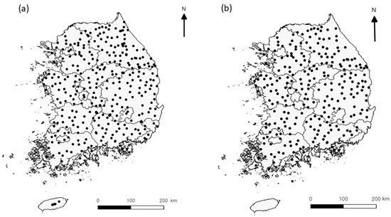
Figure 1.
Map of study sites for beetles ((a), n = 366), and spiders ((b), n = 261) in South Korea. Spider samples from high mountains (n = 105) were lost due to an accident.
For the investigation of arthropods, pitfall traps were used. Ten pitfall traps were used for each survey site. The traps were installed in a row at intervals of 5 m; the upper part of the trap was aligned with the ground surface. A white plastic cup (diameter 9.5 cm; height 6.6 cm) was used for the trap. Automobile antifreeze (propylene glycol, 100% undiluted solution) was poured into about 1/3 (about 100 mm) of the trap as a preservative. The traps were harvested 10–15 days after installation and the survey was conducted once at each site. The collected specimens were stored in the insect specimen room of the National Institute of Forest and Science. Spider specimens were identified as immersion specimens and stored in 100% ethyl alcohol; beetle specimens were identified as dry specimens. Species that were difficult to identify were classified by morpho species (e.g., Pseudoplandria sp. 1), and taxa that were difficult to classify by external morphology alone were classified into genus (e.g., Atypus spp.) or species group (e.g., Eucarabus spp. 1). The distribution data and sample photos of the species used in this study are reported in [23,24]. Of the species recorded, 52 common species were used for this study. Details of the survey site and survey method are recorded in [14,20].
2.2. Climate Data and Scenario
In previous studies [5,14,15,16,17,18,19], the temperature and precipitation were estimated based on the digital map provided by the Korea Meteorological Administration and the National Center for Agrometeorology [25]; the average from 1971 to 2008 was used. One emission scenario (SRES A1B) was used to predict the downscaled past climate. In this study, the fine-scale (30 m grid) past climate data were predicted by three climate scenarios using observational climate data of the Korea Meteorological Administration (n = 508). Three datasets were used for meteorological data: the modified special report on emission scenarios (SRES A1B) from Digital Agro-climate Map Database for Impact Assessment of Climate Change on Agriculture (http://calslab.snu.ac.kr/ncam/main; accessed on 1 September 2022) of the Rural Development Administration, South Korea, and representative concentration pathway climatic change scenarios (RCPs 4.5 and 6.0) simulated from the Climate Information Portal of the Korea Meteorological Administration (http://www.climate.go.kr; accessed on 1 September 2022). The modified SRES A1B data were generated as a regional climate model by statistically scaling down to a small scale (30 m resolution) to apply climate change scenarios to agricultural research [26,27,28]. In this study, we generated climatological normal data (1981–2010) in the study area by integrating three meteorological data sets (RCP 4.5, 6.0 and SRES A1B) to minimize variability between data sets. To evaluate the impact of climate change on the future distribution of beetles and spiders (2056–2065), the RCP 4.5 and RCP 8.5 data were used. Annual precipitation and monthly average temperatures were calculated from both climatological normal data and future climate data.
2.3. Statistical Modelling
Species distribution models were created using common species collected from more than 10% of sites (27 species of spider and 24 species of beetle). The species distribution model of abundance and occupancy (probability of presence) for the species was created using the generalized additive model (GAM). Abundance (number of individuals) was created by log transformation (ln(n + 1)) of the number of individuals in order to normalize the data and reduce variability. For occupancy analysis, abundance data were converted into binary data (0, 1) and used for analysis. In the occupancy analysis, a binomial distribution was used. The average annual temperature and annual precipitation were used as independent variables of the model. The GAM model is a non-parametric statistical model that uses a smoothing function; the fitness for data with a curved shape, such as a hump, is generally higher than that of the generalized linear model [29]. For the abundance and occupancy of each species, four GAM models were created, as follows: (1) full model—s(temp) + s(rain) + s(temp, rain), (2) two factor model—s(temp) + s(rain), (3) one and interaction factor model—s(temp) + s(temp, rain), and (4) one factor model—s(temp). Here, s(temp, rain) is the smoothing function of the interaction between the two factors. Among the four GAM models, the model with the lowest AIC (Akaike’s information criterion) value was assumed to be the optimum model and used for prediction. AIC is a statistical trade-off between log-likelihood and the number of parameters [29]. In order to determine the correlation between the prediction result and the thermal distribution, simple regression analysis was performed on the change value predicted in the model (this study and previous studies) using the species temperature index as the independent variable ([21]; STI, hereafter). The abundance-weighted STI was calculated according to the following formula: where Ai is the abundance at site i, Ti is the mean annual temperature at site i, and N is the sum of abundance of each species. The Pearson correlation was used if correlation was needed.
Future abundance and occupancy (2056–2065) were projected on the predicted temperature and precipitation for each site according to climate scenarios RCP 4.5 and 8.5 for 35 species, except for species where no significant effects of temperature and precipitation on their abundance and occupancy were observed. Using the occupancy calculated in the optimal model, the occurrence (presence 1 or absence 0) of each site was determined by species as follows: The thresholds of presence of the species were determined based on the current occupancy calculated in the model (probability of presence estimated by the model) and the number of current presence sites. Using the occurrence (0 or 1) obtained from each survey site, the future distribution for each site was predicted, and distribution changes according to latitude and altitude were analyzed based on the occurrence change. Count data was analyzed by Fisher’s exact test and chi-square test. One-way ANOVA was used to compare the values of STIs of differently responding groups (increasing, decreasing, and stable). In the case of spiders, altitude changes were not analyzed due to the loss of high mountain data. For the GAM models, R’s mgcv package was used, and for the rest of the statistical analysis, R’s stat package was used [30].
3. Results
The current average annual temperature at 366 sites is 10.3 ± 1.7 °C (5.7–13.8 °C), but, from 2056 to 2065, it is predicted to be 12.7 ± 2.5 °C (4.5–17.4 °C, RCP4.5) and 13.0 ± 2.5 °C (4.6–17.7 °C, RCP8.5). The current precipitation is 1276 ± 173 mm (964–2345 mm), but, from 2056 to 2065, it is predicted to be 1651 ± 461 mm (1130–4620 mm, RCP4.5) and 1473 ± 394 mm (972–4020 mm, RCP8.5). Thus, the precipitation is set to increase more with RCP 4.5 than with RCP 8.5. Climate change does not change evenly by space. With regard to the temperature, the temperature increases as the altitude decreases, whereas the opposite phenomenon occurs for precipitation (Figure 2).
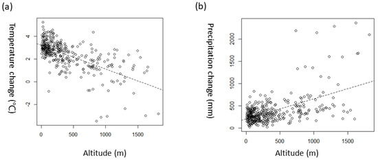
Figure 2.
Climate change (temperature and precipitation) at 366 sites in 2056-065 in South Korea according to climate change scenario RCP 4.5. Temperature is mean annual temperature. Change is the difference between the current value and the future value. The hatched lines are the fitted values of regression models ((a), Y = 3.1968 − 0.000208 × X, adj. R2 = 0.41, F1,364 = 249.8, p < 0.001; (b), Y = 204.75796 + 0.45278 × X, adj. R2 = 0.3, F1,364 = 154.8, p < 0.001).
Table 1 shows the optimum models of GAMs for the 51 species analyzed. For the adjusted R2 of the optimal model, that of the abundance of spiders was 0.1 ± 0.07 (mean ± SD, hereafter) and that of occupancy was 0.13 ± 0.11. The adjusted R2 of the abundance of beetles was 0.08 ± 0.05, and that of occupancy was 0.1 ± 0.06. The adjusted R2 of the optimal model was higher for spiders (0.11 ± 0.09) than for beetles (0.09 ± 0.05) and higher for occupancy (0.11 ± 0.09) than for abundance (0.09 ± 0.06). The species with the highest adjusted R2 value was Harmochirus insulanus, a salticid spider, with the adjusted R2 being higher than 0.3. The other three species had adjusted R2 values higher than 0.2, including Pirata yaginumai (lycosid spider), Gnaphosa kompirensis (gnaphosid spider), and Planetes (Planetes) puncticeps (carabid beetle). Among these three species, the adjusted R2’s of occupancy of Pirata yaginumai and abundance of Planetes (Planetes) puncticeps were 0.172 and 0.188, respectively, slightly lower than 0.2. For these four species with relatively high adjusted R2 values in the optimal model, the current distribution status and future changes are described in more detail in Figure 3 and Figure 4. In 12 species, including Doenitzius pruvus, Pardosa brevivulva, Orthobula crucifera, Phrurolithus pennatus, Sernokorba pallidipatellis, Xysticus ephippiatus, Asianellus festivus, Sibianor pullus, Synagelides agoriformis, Ocypus weisei, Onthophagus fodiens, Pseudocneorhinus bifasciatus, the two climatic factors did not show a significant effect on abundance or/and occupancy. These species were not analyzed for future changes, as previously described. Among the 35 species (see Table 2) that showed a significant effect of climate factors, eight species, Anahita fauna, Cladothela oculinotata, Drassyllus biglobosus, Gnaphosa kompirensis, Nicrophorus quadripunctatus, Ocypus coreanus, Pocadites sp. 1, Misolampidius tentyrioides included only temperature and 27 species included temperature and precipitation in the optimal model of abundance. In the occupancy’s optimal model, there were four species, Neoantistea quelpartensis, Itatsida praticola, Cladothela oculinotata, Drassyllus biglobosus that included only temperature and 31 species that included temperature and precipitation. These results indicate that temperature and precipitation together play an important role in the distribution and abundance of most species of arthropods. In particular, four beetle species, including Synuchus spp. 1, Synuchus spp. 2, Ocypus weisei, and Hylobius haroldi, were found to be relatively more influenced by precipitation than by temperature.

Table 1.
Optimum model of GAM (generalized additive model) uses models of 51 common species of spiders and beetles in South Korea (>10% of occurrence). The optimum model is the model with the lowest AIC values among four models (s(temp) + s(rain) + s(temp, rain), s(temp) + s(rain), s(temp) + s(temp, rain), and s(temp)) in the “mgcv” package in R. Significance, ns: p > 0.1, ^: p < 0.1, *: p < 0.05, **: p < 0.01, ***: p < 0.001. R2: adjusted R2. Abundance is a log-transformed value of captured individuals (ln(n + 1)), and occupancy is the probability of presence.
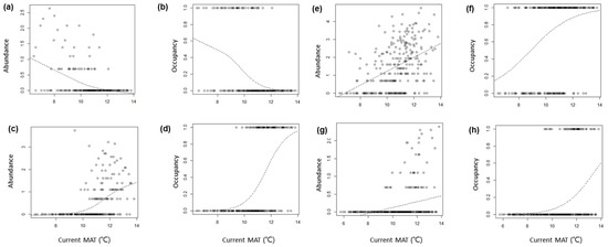
Figure 3.
Abundance (ln(n + 1)) and occupancy (probability of presence) of four species responding strongly to two climate factors (temperature and precipitation) along the temperature gradient. MAT: mean annual temperature. The hatched lines are the fitted values of GAM using MAT as the independent variable: (a,b) Gnaphosa kompirensis, (c,d) Harmochirus insulanus, (e,f) Pirata yaginumai, and (g,h) Planetes puncticeps.
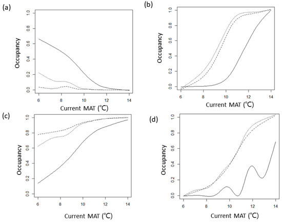
Figure 4.
Occupancy (probability of presence) in current (bold), future (2056–2065, RCP 4.5, coarsely hatched), and future (2056–2065, RCP 8.5, finely hatched) distributions along gradients of temperature (mean annual temperature) of four species highly relevant to climate factors. The lines are fitted values of the optimum models of GAM in Table 1. (a) Gnaphosa kompirensis, (b) Harmochirus insulanus, (c) Pirata yaginumai, and (d) Planetes puncticeps.
Table 2.
Abundance (ab, ln(n + 1)), probability of presence (pr), and occurrence (oc, number of occurred sites) of 35 species of spider and beetle predicted by the optimum models of GAM, as shown in Table 1. Change = future values/current values; the changes in RCP 4.5 and 8.5 are presented in [14,20]. STI: abundance weighted species temperature index, TH: threshold of presence probability for occurrence (0, 1), FD: feeding guild (n: netting, f: foraging, pr: predator, sc: scavenger, df: dung feeder, d: detritivore, pl: plant feeder). Change is qualitative change in the current study (first letter) and previous studies (second letter): i: increase, d: decrease, and s: stable. When all values of the six (current study) or two (previous studies) changes are more than 1, change is defined as i (increase). In cases less than 1, change is defined as d (decrease). When values are not coincident (> or < 1), then the values are s (stable). Family names of the species are shown in Table 1.
The abundance and distribution characteristics according to the temperature gradient of Gnaphosa kompirensis, Harmochirus insulanus, Pirata yaginumai, and Planetes puncticeps, which are highly correlated with climatic factors, are shown in Figure 3. In G. kompirensis, the abundance and occupancy decrease as temperature increases. On the other hand, the other three species (H. insulanus, P. yaginumai, and P. puncticeps) show the opposite phenomenon. These current thermal ranges are related to future distribution (Figure 3 and Figure 4). Gnaphosa kompirensis, has a distribution negatively related with temperature, decreasing at all sites as the temperature increases, while the other three species with a positive relation show an increase. However, the change in occupancy according to the temperature gradient is different for each species. Pirata yaginumai has a higher increase at lower temperature sites, but Planetes puncticeps shows a higher increase at warmer sites. On the other hand, Harmochirus insulanus has a higher increase rate at medium temperature sites. The responses to climate scenarios also differ between species. Gnaphosa kompirensis, which is expected to decrease in distribution, was found to decrease more in RCP 4.5 than in RCP 8.5. However, the three species whose distribution is expected to increase respond differently to the two climate scenarios. Harmochirus insulanus increases more in RCP 8.5, but Pirata yaginumai increases more in RCP 4.5. On the other hand, the responses to the two scenarios of Planetes puncticeps are almost identical.
Table 2 and Table 3 show the current and future abundance and distribution of 35 species that experience significant effects of climate factors. In Table 2, the values in change (RCPs 4.5 and 8.5) are the future value/current value, so values larger than 1 mean to increase, and smaller values to decrease. In Table 2, from the six change predictions, a species with all changes less than 1 is considered as a decrease (d), a species with all changes greater than 1 is considered as an increase (i), and a species with a mixture of decrease and increase is considered stable (s). Through synthesizing changes based on this, spiders showed a decrease in seven species, an increase in six species, and three species were stable. Meanwhile, beetles showed a decrease in twelve species, an increase in five species, and two species were stable (Fisher’s exact test, p = 0.06). The rate of change (average of six predictions) was 0.32 ± 0.17 for decreasing species, 2.24 ± 0.92 for increasing species, and 1.07 ± 0.33 for stable species, showing significant differences (F2,32 = 43.48, p < 0.0001). In the climate change scenario, the rate of RCP 4.5 is 0.23 ± 0.11 and that of RCP 8.5 is 0.41 ± 0.26 in the case of decreasing species, with RCP 4.5 showing a greater change. On the other hand, in the case of increasing species, RCP 4.5 is 2.17 ± 0.94 and RCP 8.5 is 2.31 ± 0.93, with RCP 8.5 showing a greater change. However, in the previous study, using only temperature, the decreasing or increasing trend was stronger in RCP 8.5 (decreasing species, RCP 4.5, 0.73 ± 0.1, RCP 8.5, 0.43 ± 0.17; increasing species RCP 4.5 1.19 ± 0.17, RCP 8.5 1.72 ± 0.66). The correlation between the temperature distribution characteristics and prediction results was confirmed by the high correlation between the STI values of 35 species and the rate of change (average of six predictions) (Table 2, Figure 5; r = 0.65, p < 0.0001). A higher correlation was found with the results of previous studies (average of RCP 4.5 and 8.5 results) that were predicted using only temperature (r = 0.78, p < 0.0001). The STI values of the 19 decreasing species were 10.09 ± 0.88 °C, while those of the 11 increasing species were 11.52 ± 0.26 °C. Those of the 5 stable species were 10.81 ± 0.99 °C, showing a significant difference among the three groups (F2,32 = 12.48, p < 0.0001). Using these characteristics, future changes can be predicted simply based on the STI value of the species. According to the regression model, in this study, if the STI value of a species was higher than 10.6 °C, the distribution and abundance of the species was expected to increase in the future, and if it was lower, it was expected to decrease. In previous studies [14,20] which made predictions using only temperature, the threshold value (10.8 °C) was slightly higher compared to this study.
Table 3.
Distribution of 35 common species of spider and beetle predicted by the optimum models in Table 1. Cu: current distribution, R4.5 and R8.5: future (2056–2065) distribution predicted according to RCP 4.5, and 8.5 climate change scenarios, respectively. MinLat: minimum latitude, MaxLat: maximum latitude, MinAlt: minimum altitude, MaxAlt: maximum altitude. Bold values indicate that the difference between future (RCP 4.5 and 8.5) and current distributions is more than one degree in latitudinal change and more than 100 m in altitudinal change. Family names of the species are shown in Table 1.
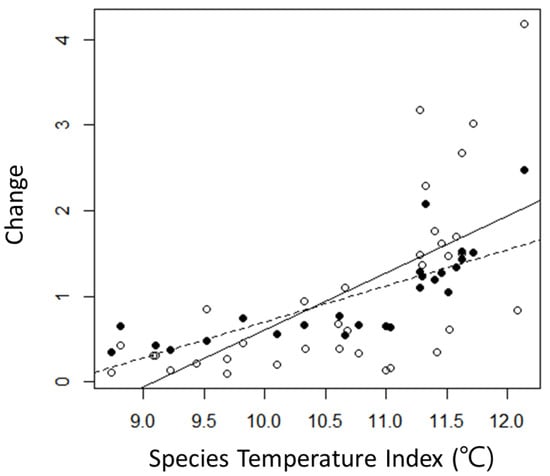
Figure 5.
Regression between species temperature index and change in distribution and abundance (average of six future changes in present study or two changes in previous studies, as shown in Table 2). White circles represent the present study, and black circles represent previous studies. The continuous line is the regression model for present studies, and the dashed line is that for other studies. Regression models: present study, Y = −6.0859 + 0.6687 × X, adj. R2 = 0.4, F1,33 = 24.02, p < 0.0001; previous studies, Y = −3.52848 + 0.42242 × X, adj. R2 = 0.59, F1,23 = 35.6, p << 0.0001.
In the results predicted by the RCP 4.5 climate scenario, local extinction (absence at all sites) was predicted for two spider species and five beetle species (Table 2). The optimal occupancy models of these seven species include precipitation. RCP 4.5 showed a greater increase in precipitation than RCP 8.5. Therefore, the local extinction of seven species is likely related to the increase in precipitation. To test this assumption, Figure 6 shows the relationship between the current occupancy of seven species and precipitation. For the sake of simplicity, only the predictions of the GAM model (occurrences(rain)) of the seven species are shown in the figure. As expected, these species show three types of hump-shaped patterns, two types in a narrow precipitation range, decreasing trends (three types), and irregular decreasing trends (two types), indicating the limited distribution of precipitation.
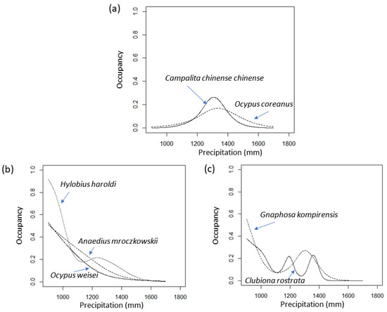
Figure 6.
Current occupancy (probability of presence) along current precipitation gradient of seven species projected to become locally extinct between 2056 and 2065 under the RCP 4.5 climate change scenario (Table 2).
The species projected to increase the most are Planetes (Planetes) puncticeps (4.19, average of six predictions) for beetles, as well as Onthophagus atripennis (3) and Evarcha albaria (3.2) and Harmochirus insulanus (2.7) for spiders. Planetes (Planetes) puncticeps, Evarcha albaria, and Harmochirus insulanus are currently not very common (frequency of occurrence: 46–83) but are predicted to become very common in the future (frequency > 200, Table 2). The species projected to decrease the most are Campalita chinense chinense (0.13), Ocypus weisei (0.13), and Anaedius mroczkowskii (0.16) for beetles, and Clubiona rostrata (0.09) and Gnaphosa kompirensis (0.1) for spiders. These species are predicted to become locally extinct (not collected from all sites) under the RCP 4.5 climate scenario (Table 2). Table 3 shows the changes in the latitude and altitude distribution of 35 species. It was assumed that a change of 1 degree or more in latitude and 100 m or more in altitude was a significant distribution change. In the case of latitude change, there were 22 species with a change in the southern limit, but 11 species with a change in the northern limit (χ 2 = 3.67, p = 0.056). However, in the case of altitude (beetles only), there were many species with varying highest elevations, with 19 species changing to their highest elevation, compared to 7 species changing to their lowest elevation of the distribution (χ 2 = 5.54, p = 0.019).
There is a very high relation between the abundance and occurrence of 35 species (Figure 7). In order to test the positive correlation between abundance and distribution, the results of calculating abundance only at the sites where each species appeared are shown in Figure 7b. As expected, a positive correlation appears, but there is a slight difference in the slope and adjusted R2 value of the regression models between beetles and spiders. Beetles had a higher slope value and a higher adjusted R2 value than spiders. There is a very high correlation between abundance and occupancy and between occupancy and occurrence. In the latter case, beetles show a lower slope than spiders in the regression equation.
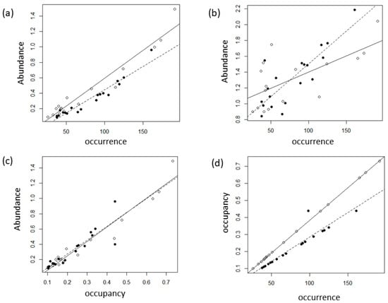
Figure 7.
Regression between abundance (ln(number of individuals +1)), occurrence (number of sites occurring), and occupancy (probability of presence) of 35 species of spiders and beetles. Data are the average of each species (Table 2). The white circles are spiders, and the black circles are beetles. The continuous lines are the regression models for spiders, and the dashed lines are those of beetles. Regression models, (a) abundance at all sites, spiders, Y = −0.130232 + 0.0072343 × X, adj. R2 = 0.94, F1,14 = 228.8, p < 0.0001, beetles, Y = −0.1650507 + 0.0060726 × X, adj. R2 = 0.93, F1,17 = 231.5, p < 0.0001; (b) abundance at occurred sites, spiders, Y = 0.98294 + 0.004109 × X, adj. R2 = 0.4, F1,14 = 10.95, p = 0.005, beetles, Y = 0.673866 + 0.008289 × X, adj. R2 = 0.68, F1,17 = 39.79, p < 0.0001; (c) spiders, Y = −0.13023 + 1.88816 × X, adj. R2 = 0.94, F1,14 = 228.8, p < 0.0001, beetles, Y = −0.09522 + 1.82075 × X, adj. R2 = 0.78, F1,17 = 64.86, p < 0.0001; and (d) spiders, Y = 0.00381 × X, adj. R2 = 1, F1,14 = 3.778e + 17, p < 0.0001, beetles, Y = −0.0022437 + 0.0028 × X, adj. R2 = 0.87, F1,17 = 118.2, p < 0.0001.
4. Discussion
In a two-dimensional prediction using temperature and precipitation, the range of change was larger compared with a one-dimensional prediction using temperature. The intensity of the change was more severe in this study than in previous studies [14,20]. Projections of this study showed that the decreasing species in future decreased more and the increasing species increased more. In the case of response to the climate change scenario, more changes occurred in RCP 8.5, with a large increase in temperature in the prediction using only temperature, but greater decrease in RCP 4.5 in the case of decreasing species when temperature and precipitation were used for prediction. This is assumed to be related to the tendency of RCP 4.5 to increase precipitation more than RCP 8.5. Four beetle species, including Synuchus spp 1, Synuchus spp. 2, Ocypus weisei, and Hylobius haroldi, for which precipitation had a greater effect on abundance and distribution than temperature, are predicted to decrease, and this decrease is larger in RCP 4.5 than RCP 8.5, showing the strong influence of precipitation. In addition, the fact that all seven species predicted to be locally extinct in RCP 4.5 are species that have a negative relation with precipitation, or inhabit a narrow range of precipitation, make this finding even clearer. In general, it is expected that the distribution change will be larger in a climate change scenario with a large increase in temperature. However, when including precipitation, the results forecast are more complicated. In this study, the explanation of the variation in the species distribution models using temperature and precipitation was about 10%, which was low. However, even in complex regression models including seven environmental factors (i.e., NDVI, light intensity, altitude, and four climate factors), the value of the adjusted R2 was not higher than that of this study ([17], beetle 0.065 ± 0.038, n = 18; [14], spider 0.11 ± 0.055, n = 19). In the regression models of previous studies, one reason for the low adjusted R2 value is that the non-linearity (curve) between climate factors and abundance was not reflected. Thus, the low adjusted R2 value of the distribution models obtained from the current distribution data indicates the limitation of predicting the future using the current distribution data. In addition, the uncertainty of the climate change scenario itself also plays a prominent role in increasing the uncertainty of the forecast. The climate change scenario largely depends on the global economic situation, technological development, and climate change response policies, but it is difficult to predict any of these, and the uncertainty is very high [31]. Therefore, it is believed that more significance should be given to the qualitative trend (decrease or increase, etc.) rather than the quantitative aspect of the prediction results for distribution and abundance change.
The adjusted R2 value of the distribution models was a little higher for spiders than for beetles, and for occupancy rather than for abundance. Since this study was conducted at many sites, only one survey could be conducted. If the survey was conducted in the non-adult period of a species, the species was not collected. Therefore, the longer the adult period, the lesser the false absence, which will increase the fitness (adjusted R2 value) of the distribution model. Therefore, the adult period of spiders is somewhat longer than that of beetles [32], which is considered the cause of the increased fitness of the spider distribution models. In the case of the ants collected in this study, the adjusted R2 value was 0.18 ± 0.16 (21 species, n = 42), which is much higher than that of beetles and spiders (unpublished data). In the case of ants, since worker ants forage from the end of April to the end of October, the collection is less limited by the sampling period than that of spiders or beetles. In general, when predicting distribution changes due to climate change, occurrence is predicted rather than abundance (e.g., [2]). The reason for this is that the data used for distribution prediction are obtained from various sources (museum specimens, literature, etc.) rather than a standardized survey, such as in this study. Another reason is that occurrence is easier to predict than abundance. In order to predict species richness or distribution changes (latitude, altitude, etc.), occurrence rather than abundance is needed. In this study, the adjusted R2 value is higher in occurrence than abundance, confirming existing results, but the difference is not high. The patterns of the two population variables according to the temperature gradient are also similar. Additionally, there is a high correlation between abundance and occupancy (probability of presence) obtained from binary data (0 or 1). This means that, when monitoring at many sites, as carried out in this study, abundance can be accurately inferred using the obtained regression model, even if only occurrence is recorded without counting abundance, which requires much effort. It is also important to confirm the positive correlation between distribution (occurrence) and abundance in this study. The phenomenon that “the wider the distribution, the higher the abundance” is an ecological phenomenon found in almost all taxa and all regions [33]. This is confirmed by spiders and beetles in South Korea, in which there are no previous studies on this phenomenon. There is a report that the slope of the regression model between occurrence and abundance changes as the environment changes [34]. Therefore, the results obtained in this study (Figure 7b) can be used as baseline data for future studies to indicate changes in arthropod communities in South Korea due to climate changes.
If the distribution of organisms moves northward due to climate warming, the abundance and distribution of northern species that are adapted to cold northern regions decrease in temperate regions such as Korea, and southern species adapted to hot southern regions also decrease [35]. It is STI that quantifies this qualitative concept. The STI is either simply calculated as the average of the mean annual temperature of the collection sites, or by reflecting the abundance, as in this study. Kwon (2017) [36] reported that there was little difference between the former and the latter using ants. The STI, which shows the temperature distribution characteristics of species, is low for northern species living in cold regions and high for southern species living in warm regions. This can be confirmed from the observation that the STI value of the species expected to decrease in this study is lower than the STI value of the species expected to increase. The correlation between the change value of the previous studies using only temperature and STI was higher than that of this study using temperature and precipitation. This means that, as expected, when temperature and precipitation are used, the effect of the temperature distribution characteristics of the species on the change value is reduced. Based on the regression model between STI and change obtained in this study, it is predicted that a species will decrease if its STI value is lower than 10.6 °C and increase if it is higher. The threshold value of STI in the previous studies was 10.8 °C. These values are slightly higher than the average of the mean annual temperature of all sites: 10.3 °C. If the mean annual temperature at which the abundance of a certain species is maximum (optimal temperature) is known, future changes can be estimated by comparing MAT in a region and the optimal temperature [20]. For example, if the optimum temperature of species A is 10.2 °C and the MAT of a region is 9 °C, the species will increase in the future. In a region with a MAT of 11 °C, the species will decrease. Theoretically, the STI should be the optimum temperature, but, in practice, it is not. The STI obtained in a narrow area such as South Korea is higher than the optimum temperature for northern species and lower for southern species. The average value of the STI values of the species collected from one site is the community temperature index [21]. Due to the bias in the STI value, the slope of the regression model of CTI and MAT becomes lower [20]. The slope value of this regression model is used to calculate the distribution change from the CTI value change [21]. However, the bias of the STI value does not affect the distribution change calculation [21]. As the temperature increases, the species with low STI values decrease in distribution and abundance in a region, and those with high STI values increase, increasing the CTI value of the region. Through this method, it is possible to test the impact of climate change due to temperature increase, such as community change or distribution change [21,37,38]. Based on the distribution change of species obtained in this study, the CTI change can be predicted.
By predicting the distribution of spiders and beetles based on occurrence changes, it was predicted that future distributional changes would cause changes in altitude rather than in latitude in the case of beetles. This is a naturally expected result due to the small area of South Korea. According to climate change scenario RCP 4.5, local extinctions of seven species are predicted. The number of occurrence sites of these species is between 33 and 69, which is not very common. The STI values (8.7–10.1 °C) of Clubiona rostrata, Gnaphosa kompirensis, Campalita chinense chinense, and Ocypus coreanus were lower than the average value of the MAT of all survey sites (10.3 °C), but the STI values of Ocypus weisei and Anaedius mroczkowskii were high (11 °C). These two species were predicted to become locally extinct due to increased precipitation despite their high STI values, as previously described. Since Ocypus coreanus and Anaedius mroczkowskii are endemic to Korea [39], conservation measures are necessary to prevent the local extinction of these species.In particular, A. mroczkowskii is a detritivore so it plays an important role in the forest by consuming detritus. On the other hand, the four species that are expected to benefit the most from climate change are Evarcha albaria, Harmochirus insulanus, Planetes (Planetes) puncticeps, and Onthophagus atripennis. These species are not very common now (47–91 occurrences) but are projected to become very common in the future (170–215 occurrences). In Onthophagus atripennis, the increase in abundance was expected to be much greater than that of occurrence. Since this species feeds on mammalian dung [40], the influence of changes in mammalian abundance will be important for this species. Planetes (Planetes) puncticeps inhabit forests, forest edges and fields [41]. Overseas, it is distributed in Japan, China and Taiwan, and, in Korea, it is recorded in Mt. Chiak, Mt. Palgong, Mt. Namjang, Mt. Muak, Geoje, and Jindo [42]. Evarcha albaria is distributed nationwide and is commonly observed in forests, grasslands, and around private houses; the adult season lasts from May to September. Overseas distributions are Japan, China, Mongolia, and Russia [32]. The adult season of Harmochirus insulanus is June–September, and it is active in the vegetation layer [43].
34t is distributed nationwide, and its overseas distribution is Japan, China, India, and Australia [32]. These three species are predators that will be affected by the abundance and distribution of their prey and can also affect the abundance and distribution of the prey. Two species described in [14], including Diplocephaloides saganus and Nippononeta cheunghensis, were identified in this study as the female and male of Syedra oii, respectively. In [14], two misidentified species were predicted to decrease, but, in this study, Syedra oii was predicted to show little change (abundance slightly increased; distribution slightly decreased).
As a result of two-dimensional prediction using precipitation and temperature, the range of change was larger than that of one-dimensional prediction using only temperature. The concomitant increase along with the increase in temperature was found to have a significant effect on the change in distribution and abundance of arthropods. Arthropods are important as indicators of climate change due to their high number of species, good mobility, and physiological characteristics that are absolutely dependent on temperature [35,44,45]. For this reason, the National Institute of Forest Science is monitoring arthropods at about 300 forest sites nationwide every five years [46]. This study analyzes the results of the first survey. Beetles and spiders are very promising indicators of climate change, but too many species and difficult classification are the biggest challenges for research. Due to the re-identification of beetle identification findings compiled in the first survey (2006–2009) by coleopteran taxonomists, the identification agreement rate was only 20% [43]. In addition, there were many cases where one species was classified as several species, or several species were classified as one species [43]. The best method is that many experts identify the collected specimens in their taxa, but, in practice, this is difficult to carry out. In the case of spiders, one species was identified as two different species, as described above, even though they were identified by a spider taxonomist. To overcome this difficulty, some of the common species that were accurately identified, even by non-specialists, and being amenable to statistical analysis due to abundance, can be utilized as indicators of the influence of climate change. One of the implicit purposes of this study is to select the climate change indicator species. Among the species predicted in this study, those that are easy to identify will be promising indicators of climate change. Because of the low effectiveness of the species distribution models and the uncertainty of the climate change scenario, it is very difficult to quantitatively predict the future of a population, but qualitative changes (increase or decrease) are easier to predict. Therefore, the most important thing in climate change research is standardized long-term monitoring rather than uncertain predictions using models. Data from such monitoring can be used to recognize the direction of change, greatly aiding the conservation of vulnerable global biodiversity.
Author Contributions
Conceptualization, T.-S.K.; methodology, T.-S.K.; software, T.-S.K.; validation, T.-S.K., and Y.N.; formal analysis, T.-S.K.; investigation, T.-S.K. and S.-S.K.; resources, T.-S.K. and Y.N.; data curation, T.-S.K.; writing—original draft preparation, T.-S.K.; writing—review and editing, T.-S.K., W.I.C. and Y.N.; visualization, T.-S.K.; supervision, T.-S.K.; project administration, Y.N.; funding acquisition, Y.N. All authors have read and agreed to the published version of the manuscript.
Funding
This study was supported by the National Institute of Forest Science (project No.: FE0703-2022-01-023 and FE0100-2023-02-2023), Republic of Korea.
Institutional Review Board Statement
Not applicable.
Informed Consent Statement
Not applicable.
Data Availability Statement
The data presented in this study are available on request from the corresponding author. The data are not publicly available due to institutional policy.
Conflicts of Interest
The authors declare no conflict of interest.
References
- Im, M.-S. The Spiders of Korea; Ji-Gu Publishing Co.: Seoul, Republic of Korea, 1996; p. 249. (In Korean) [Google Scholar]
- Peterson, A.T.; Ortega-Huerta, M.A.; Bartley, J.; Sanches-Cordero, V.; Soberan, J.; Buddemeier, R.H.; Stockwell, D.R.B. Future projections for Mexican faunas under global climate change scenarios. Nature 2002, 416, 626–628. [Google Scholar] [CrossRef] [PubMed]
- Walther, G.-R.; Post, E.; Convey, P.; Menzels, A.; Parmesan, C.; Beebee, T.J.C.; Fromentin, O.; Hoegh-Guldberg, J.M.; Bairlein, F. Ecological responses to recent climate change. Nature 2002, 416, 389–395. [Google Scholar] [CrossRef] [PubMed]
- Cheung, W.W.L.; Lam, V.W.Y.; Sarmiento, J.L.; Kearney, K.; Watson, R.; Pauly, D. Projecting global marine biodiversity impacts under climate change scenarios. Fish Fish. 2009, 10, 235–251. [Google Scholar] [CrossRef]
- Kwon, T.-S.; Lee, C.M. Prediction of abundance of ants according to climate change scenario RCP 4.5 and 8.5 in South Korea. J. Asia-Pac. Biodivers. 2015, 8, 49–65. [Google Scholar] [CrossRef]
- Thomas, C.D.; Cameron, A.; Green, R.E.; Bakkenes, M.; Beaumont, L.J.; Collingham, Y.C.; Erasmus, B.F.N.; de Siqueira, M.F.; Grainger, A.; Hannah, L.; et al. Extinction risk from climate change. Nature 2004, 427, 145–148. [Google Scholar] [CrossRef]
- Thuiller, W. BIOMOD-optimizing predictions of species distributions and projecting potential future shifts under global change. Glob. Chang. Biol. 2003, 9, 1353–1362. [Google Scholar] [CrossRef]
- Beaumont, L.J.; Hughes, L.; Poulsen, M. Predicting species distributions: Use of climatic parameters in BIOCLIM and its impact on predictions of species’ current and future distributions. Ecol. Model. 2005, 186, 251–270. [Google Scholar] [CrossRef]
- Bewick, S.; Stuble, K.L.; Lessard, J.-P.; Dunn, R.R.; Adler, F.R.; Sanders, N.J. Predicting future coexistence in a North American ant community. Ecol. Evol. 2014, 4, 1804–1819. [Google Scholar] [CrossRef]
- Şen, I.; Sarıkaya, O.; Örücü, Ö.K. Predicting the future distributions of Calomicrus apicalis Demaison, 1891 (Coleoptera: Chrysomelidae) under climate change. J. Plant Dis. Prot. 2022, 129, 325–337. [Google Scholar] [CrossRef]
- Avtaeva, T.A.; Sukhodolskaya, R.A.; Brygadyrenko, V.V. Modeling the bioclimatic range of Pterostichus melanarius (Coleoptera, Carabidae) in conditions of global climate change. Biosyst. Divers. 2021, 29, 140–150. [Google Scholar] [CrossRef]
- Li, A.; Wang, J.; Wang, R.; Yang, H.; Yang, W.; Yang, C.; Jin, Z. MaxEnt modeling to predict current and future distributions of Batocera lineolata (Coleoptera: Cerambycidae) under climate change in China. Ecoscience 2020, 27, 23–31. [Google Scholar] [CrossRef]
- Saupe, E.E.; Papes, M.; Selden, P.A.; Richard, S.; Vetter, R.S. Tracking a medically important spider: Climate change, ecological niche modeling, and the Brown Recluse. PLoS ONE 2011, 6, e17731. [Google Scholar] [CrossRef] [PubMed]
- Kwon, T.-S.; Lee, C.M.; Kim, T.W.; Kim, S.-S.; Sung, J.H. Prediction of abundance of forest spiders according to climate warming in South Korea. J. Asia-Pac. Biodivers. 2014, 7, e133–e155. [Google Scholar] [CrossRef]
- Kwon, T.-S.; Lee, C.M.; Park, J.; Kim, S.-S.; Chun, J.H.; Sung, J.H. Prediction of abundance of ants due to climate warming in South Korea. J. Asia-Pac. Biodivers. 2014, 7, 179–196. [Google Scholar] [CrossRef]
- Kwon, T.-S.; Li, F.; Kim, S.-S.; Chun, J.H.; Park, Y.-S. Modelling vulnerability and range shifts in ant communities responding to future global warming in temperate forests. PLoS ONE 2016, 11, e0159795. [Google Scholar] [CrossRef] [PubMed]
- Kwon, T.-S.; Lee, C.M.; Kim, S.-S. Prediction of abundance of beetles according to climate warming in South Korea. J. Asia-Pac. Biodivers. 2015, 8, 7–30. [Google Scholar] [CrossRef]
- Lee, C.M.; Kwon, T.-S.; Kim, S.-S.; Park, G.-E.; Lim, J.-H. Prediction of abundance of arthropods according to climate change scenario RCP 4.5 and 8.5 in South Korea. J. Asia-Pac. Biodivers. 2016, 9, 116–137. [Google Scholar] [CrossRef]
- Lee, C.M.; Kwon, T.-S.; Ji, O.Y.; Kim, S.-S.; Park, G.-E.; Lim, J.-H. Prediction of abundance of forest flies (Diptera) according to climate scenarios RCP 4.5 and RCP 8.5 in South Korea. J. Asia-Pac. Biodivers. 2015, 8, 349–370. [Google Scholar] [CrossRef]
- Kwon, T.-S. Change of ant fauna in the Gwangneung forest: Test on influence of climatic warming. J. Asia-Pac. Biodivers. 2014, 7, 219–224. [Google Scholar] [CrossRef]
- Devictor, V.; Julliard, R.; Couvet, D.; Jiguet, F. Birds are tracking climate warming, but not fast enough. Proc. R. Soc. B Biol. Sci. 2008, 275, 2743–2748. [Google Scholar] [CrossRef] [PubMed]
- Kwon, T.-S.; Kim, S.-S.; Chon, J.H. Pattern of ant diversity in Korea: An empirical test of Rapoport’s altitudinal rule. J. Asia-Pac. Entomol. 2014, 17, 161–167. [Google Scholar] [CrossRef]
- Kwon, T.-S.; Lee, C.M.; Kim, B.W.; Kim, T.U.; Kim, S.-S.; Sung, J.H. Prediction of Distribution and Abundance of Forest Spiders according to Climate Scenario RCP 4.5 and 8.5; Research Note 528; Korea Forest Research Institute: Seoul, Republic of Korea, 2013. [Google Scholar]
- Kwon, T.-S.; Lee, C.M.; Kim, S.-S.; Chun, J.H.; Lee, Y.G.; Sung, J.H.; Lim, J.H. Prediction of Abundance of Beetle Populations Based on RCP 4.5 and 8.5 Climate Scenario in South Korea; Research Note 554; Korea Forest Research Institute: Seoul, Republic of Korea, 2014. [Google Scholar]
- Yun, J.I.; Kim, J.H.; Kim, S.O.; Kwon, T.S.; Chon, J.H.; Sung, J.H.; Lee, Y.G. Development of Digital Climate Map of Korean Forest and Prediction of Forest Climate; Research Report 13–19; Korea Forest Research Institute: Seoul, Republic of Korea, 2013. [Google Scholar]
- Chung, N.; Kwon, Y.-S.; Li, F.; Bae, M.-J.; Chung, E.G.; Kim, K.; Lee, S.; Hwang, S.-J.; Park, Y.-S. Basin specific effect of global warming on the distribution of endemic riverine fish in Korea: Implication for biodiversity conservation. Ann. Limnol.-Int. J. Lim. 2016, 52, 171–186. [Google Scholar] [CrossRef]
- Yun, J.I. Application of high dimension digital climate maps in restructuring of Korean agriculture. Korean J. Agric. For Meteorol. 2007, 9, 1–16. [Google Scholar] [CrossRef]
- Yun, J.I. Agroclimatic maps augmented by a GIS technology. Korean J. Agric. For Meteorol. 2010, 12, 63–73. [Google Scholar] [CrossRef]
- Crawley, M.J. The R Book, 1st ed.; John Wiley & Sons, Ltd.: Chichester, UK, 2007. [Google Scholar]
- R Core Team. R: A Language and Environment for Statistical Computing; R Foundation for Statistical Computing: Vienna, Austria, 2020; Available online: https://www.R-project.org/ (accessed on 1 April 2020).
- Pachauri, R.K.; Allen, M.R.; Barros, V.R.; Broome, J.; Cramer, W.; Christ, R.; Church, J.A.; Clarke, L.; Dahe, Q.D.; Dasqupta, P.; et al. Climate Change 2014: Synthesis Report; Contribution of Working Groups I, II and III to the Fifth Assessment Report of the Intergovernmental Panel on Climate Change; IPCC: Geneva, Switzerland, 2014. [Google Scholar]
- Namkung, J. The Spiders of Korea, 2nd ed.; Kyo-Hak Publishing Co., Ltd.: Seoul, Republic of Korea, 2003. (In Korean) [Google Scholar]
- Gaston, K.J.; Curnutt, J.L. The dynamics of abundance-range size relationships. Oikos 1998, 81, 38–44. [Google Scholar] [CrossRef]
- Frisk, M.G.; Duplisea, D.E.; Trenkel, V.M. Exploring the abundance-occupancy relationships for the Georges Bank finfish and shellfish community from 1963 to 2006. Ecol. Appl. 2011, 21, 227–240. [Google Scholar] [CrossRef]
- Kwon, T.-S.; Kim, S.-S.; Chun, J.H.; Byun, B.K.; Lim, J.H.; Shin, J.H. Changes in butterfly abundance in response to global warming and reforestation. Environ. Entomol. 2010, 39, 337–345. [Google Scholar] [CrossRef]
- Kwon, T.-S. Temperature and ant assemblages: Biased values of community temperature index. J. Asia-Pac. Entomol. 2017, 20, 1077–1086. [Google Scholar] [CrossRef]
- Jiguet, F.; Brotons, L.; Devictor, V. Community responses to extreme climatic conditions. Curr. Zool. 2011, 57, 406–413. [Google Scholar] [CrossRef]
- Roth, T.; Plattner, M.; Amrhein, V. Plants, birds and butterflies: Short-term responses of species communities to climate warming vary by taxon and with altitude. PLoS ONE 2014, 9, e82490. [Google Scholar] [CrossRef]
- Nam, G.H.; Lee, B.Y.; Kwak, M.H.; Lim, C.K.; Kim, C.H.; Han, K.D.; Go, E.S. Endemic Species of Korea; National Institute of Biological Resources: Incheon, Republic of Korea, 2011; p. 451. [Google Scholar]
- Ueno, S.-I.; Kurosawa, Y.; Sato, M. The Coleoptera of Japan in Color, 3rd ed.; Hoihusa Publishing Co., Ltd.: Osaka, Japan, 1989. (In Japanese) [Google Scholar]
- Lake Biwa Museum. Ground Beetles of Satoyama, Shiga, Japan. 2014. Available online: http://www.lbm.go.jp/emuseum/zukan/gomimushi/index.html (accessed on 1 September 2022).
- Park, J.K.; Paik, J.C. Family Carabidae. Economic insects of Korea 12. Ins. Koreana Suppl. 2001, 30, 99. (In Korean) [Google Scholar]
- Kwon, T.-S.; Park, S.; Lee, S.-G.; Kim, L.; Nam, Y. Coleoptera (Except Carabidae) Specimen in National Institute of Forest Science; Research Note 802; National Institute of Forest Science: Seoul, Republic of Korea, 2019. [Google Scholar]
- Andrew, N.R.; Hughes, L. Arthropod community structure along a latitudinal gradient: Implications for future impacts of climate change. Austral. Ecol. 2005, 30, 281–297. [Google Scholar] [CrossRef]
- Uvarov, B.P. Insects and climate. Trans. Ent. Soc. Lond. 1931, 79, 1–232. [Google Scholar] [CrossRef]
- Lim, J.; Park, G.; Won, M.; Kim, E.; Jang, G.; Yang, H.; Kim, S.; Chun, J.; Park, C.; Choi, H.; et al. Guidelines for Survey and Assessment of Climate Change Impacts in Forestry and Forest; Research Note 740; National Institute of Forest Science: Seoul, Republic of Korea, 2017. [Google Scholar]
Disclaimer/Publisher’s Note: The statements, opinions and data contained in all publications are solely those of the individual author(s) and contributor(s) and not of MDPI and/or the editor(s). MDPI and/or the editor(s) disclaim responsibility for any injury to people or property resulting from any ideas, methods, instructions or products referred to in the content. |
© 2023 by the authors. Licensee MDPI, Basel, Switzerland. This article is an open access article distributed under the terms and conditions of the Creative Commons Attribution (CC BY) license (https://creativecommons.org/licenses/by/4.0/).