
Land Use and Land Cover Trends and Their Impact on Streamflow and Sediment Yield in a Humid Basin of Brazil’s Atlantic Forest Biome

 , ,
, ,  ,
,  , ,
, ,  and
and 
Abstract
:1. Introduction
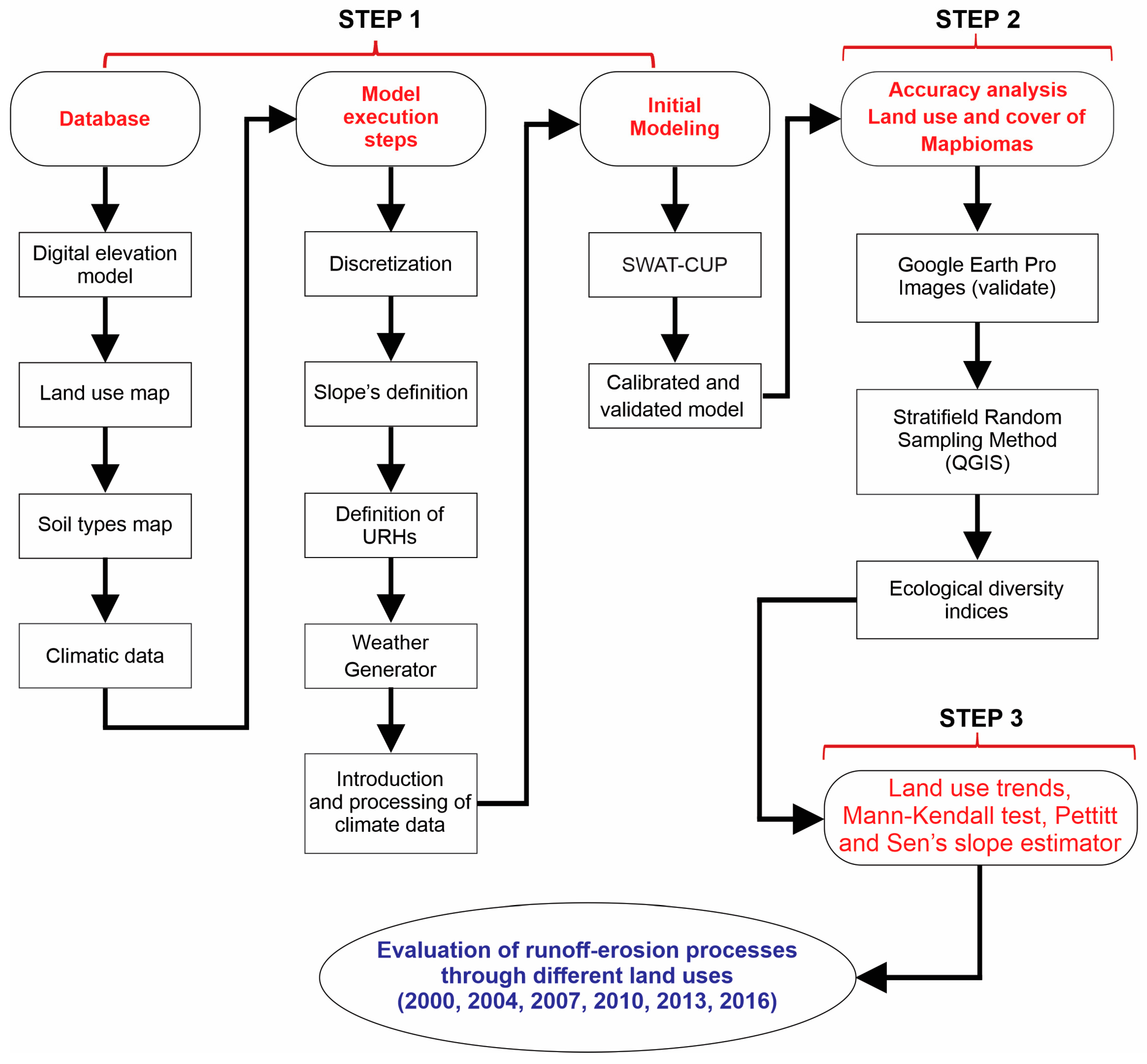
2. Materials and Methods
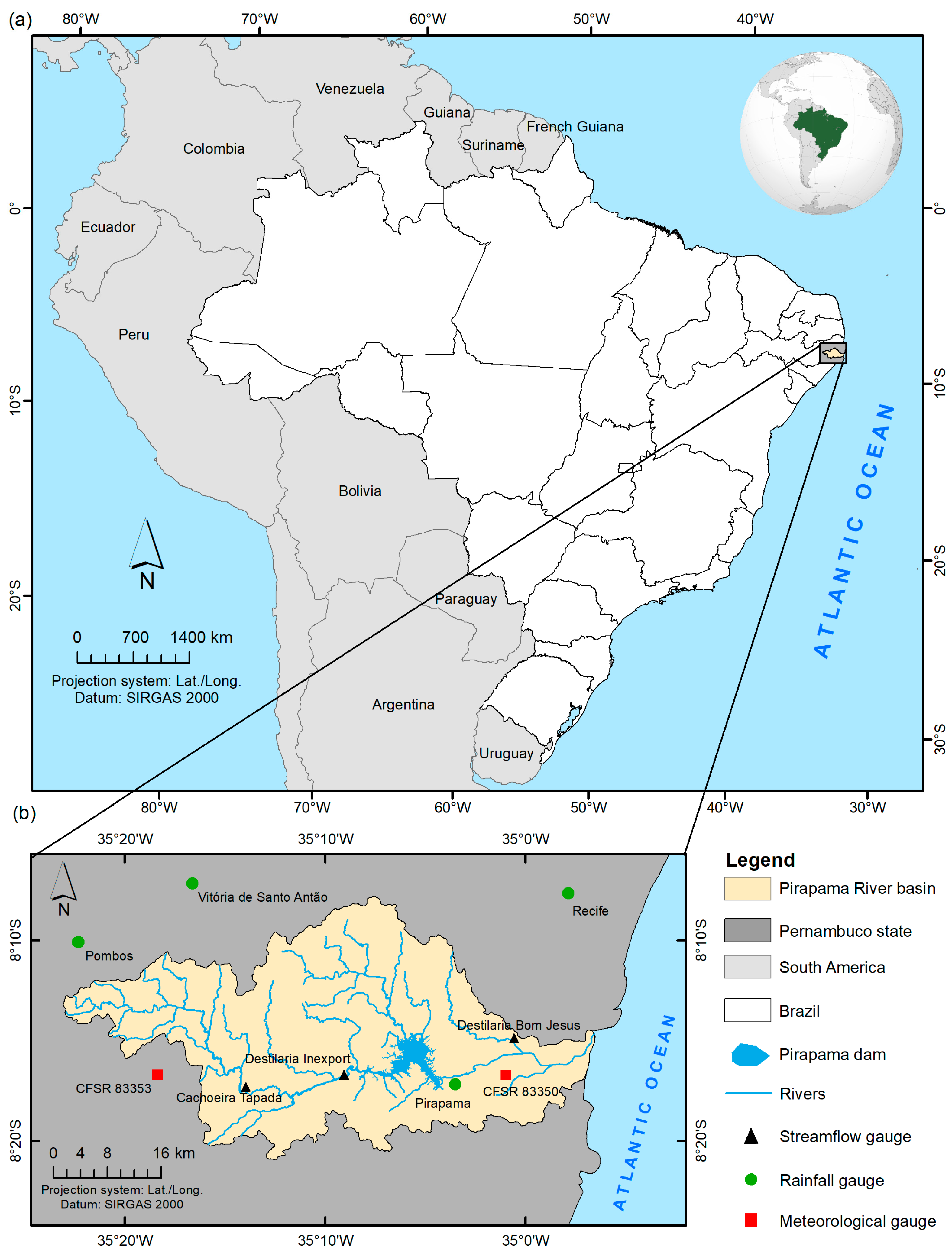
2.1. Study Area
2.2. Land Use and Land Cover Dataset
2.3. Accuracy Assessment of LULC
2.4. LULC Trend Analysis
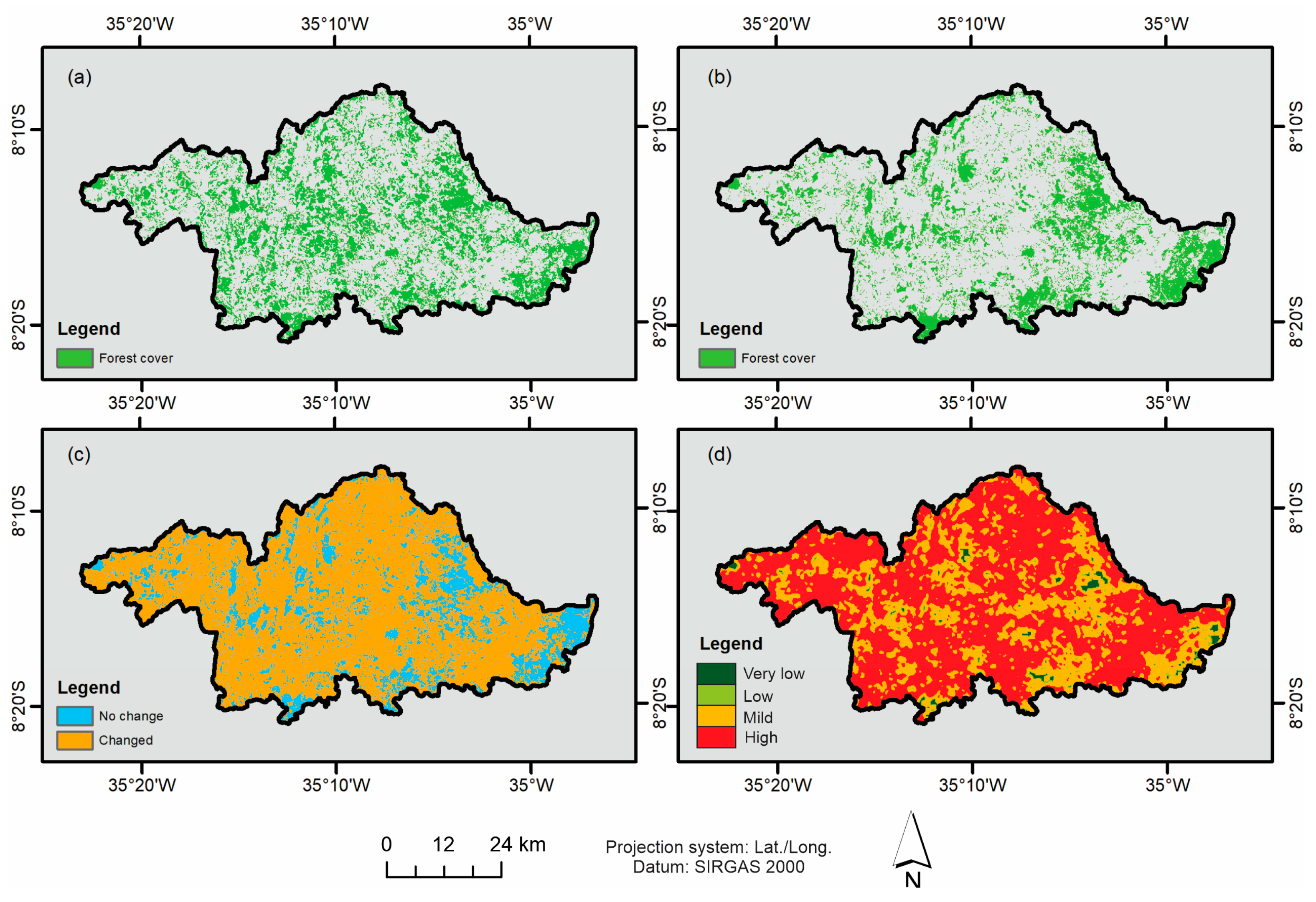
2.5. Forest Fragmentation Analysis
2.6. Streamflow and Sediment Yield Simulation
2.6.1. SWAT Input Database
2.6.2. Meteorological Data
2.6.3. Calibration and Validation of the SWAT Model
2.6.4. Performance Indices of Hydrologic Modeling
2.7. Evaluation of Streamflow and Sediment Yield
3. Results
3.1. LULC Change Analysis
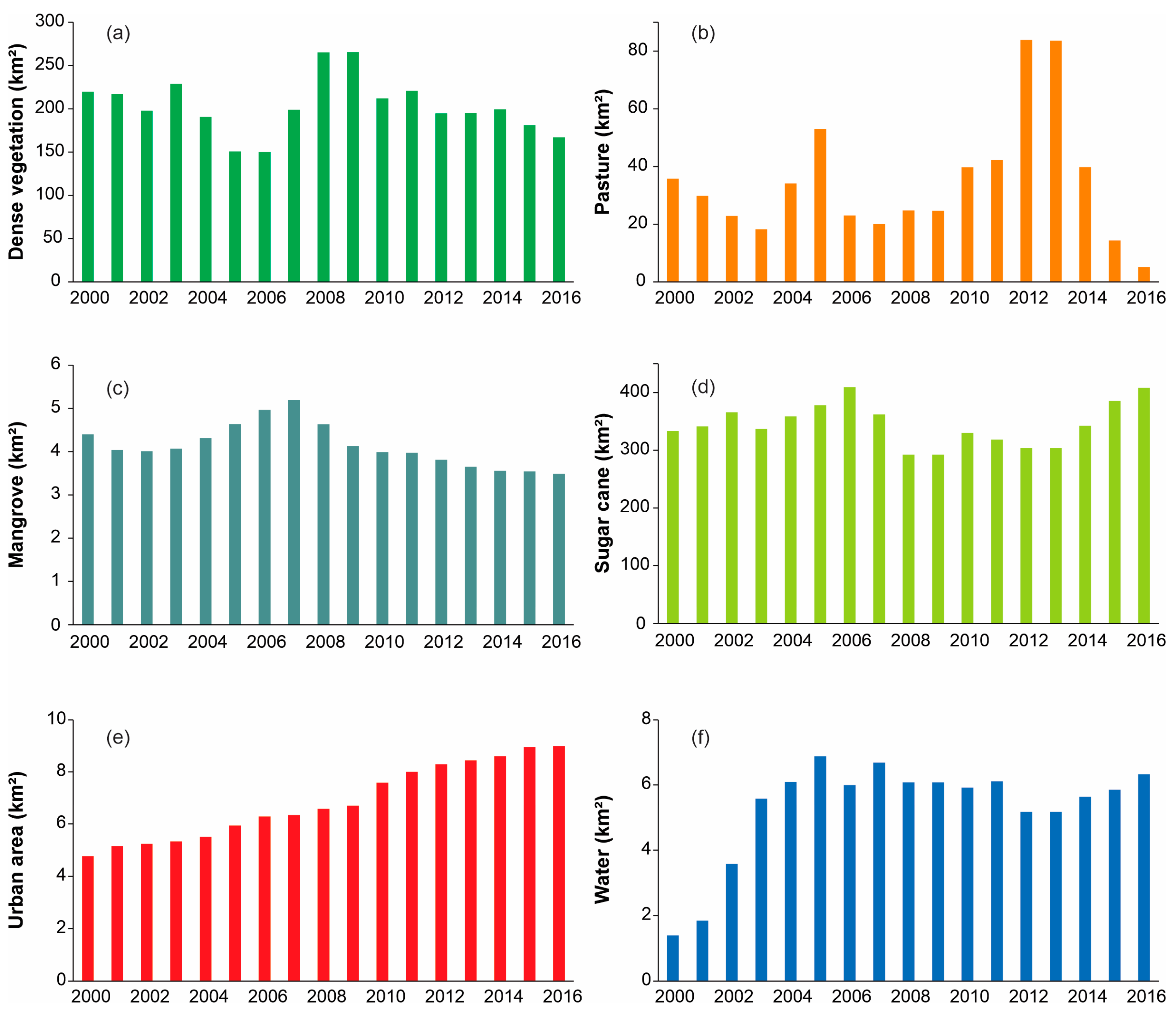
3.2. Trends in LULC Evolution
3.3. Analysis of Streamflow for Different LULC Scenarios
3.4. Hydrological Balance Analysis for Different LULC Scenarios
4. Discussion
4.1. Limitations, Advantages, and Applications of the Study
4.2. Impacts of LULC Changes on Sediment Yield
5. Conclusions
Author Contributions
Funding
Data Availability Statement
Conflicts of Interest
References
- Loiselle, D.; Du, X.; Alessi, D.S.; Bladon, K.D.; Faramarzi, M. Projecting impacts of wildfire and climate change on streamflow, sediment, and organic carbon yields in a forested watershed. J. Hydrol. 2020, 590, 125403. [Google Scholar] [CrossRef]
- Yin, S.; Gao, G.; Li, Y.; Xu, Y.J.; Turner, R.E.; Ran, L.; Wang, X.; Fu, B. Long-term trends of streamflow, sediment load and nutrient fluxes from the Mississippi River Basin: Impacts of climate change and human activities. J. Hydrol. 2023, 616, 128822. [Google Scholar] [CrossRef]
- Juma, L.A.; Nkongolo, N.V.; Raude, J.M.; Kiai, C. Assessment of hydrological water balance in Lower Nzoia Sub-catchment using SWAT-model: Towards improved water governace in Kenya. Heliyon 2022, 8, e09799. [Google Scholar] [CrossRef] [PubMed]
- Huq, E.; Abdul-Aziz, O.I. Climate and land cover change impacts on stormwater runoff in large-scale coastal-urban environments. Sci. Total Environ. 2021, 778, 146017. [Google Scholar] [CrossRef] [PubMed]
- Wang, L.; Hou, H.; Li, Y.; Pan, J.; Wang, P.; Wang, B.; Chen, J.; Hu, T. Investigating relationships between landscape patterns and surface runoff from a spatial distribution and intensity perspective. J. Environ. Manag. 2023, 325, 116631. [Google Scholar] [CrossRef] [PubMed]
- Rápalo, L.M.C.; Uliana, E.M.; Moreira, M.C.; da Silva, D.D.; Ribeiro, C.B.M.; da Cruz, I.F.; Pereira, D.R. Effects of land-use and -cover changes on streamflow regime in the Brazilian Savannah. J. Hydrol. Reg. Stud. 2021, 38, 100934. [Google Scholar] [CrossRef]
- Zhao, C.S.; Yang, Y.; Yang, S.T.; Xiang, H.; Wang, F.; Chen, X.; Zhang, H.M.; Yu, Q. Impact of spatial variations in water quality and hydrological factors on the food-web structure in urban aquatic environments. Water Res. 2019, 153, 121–133. [Google Scholar] [CrossRef]
- Zema, D.A.; Lucas-Borja, M.E.; Carrà, B.G.; Denisi, P.; Rodrigues, V.A.; Ranzini, M.; Arcova, F.C.S.; de Cicco, V.; Zimbone, S.M. Simulating the hydrological response of a small tropical forest watershed (Mata Atlantica, Brazil) by the AnnAGNPS model. Sci. Total Environ. 2018, 636, 737–750. [Google Scholar] [CrossRef]
- Feitosa, T.B.; Fernandes, M.M.; Santos, C.A.G.; Silva, R.M.; Garcia, J.R.; Araujo Filho, R.N.; Fernandes, M.R.M.; Cunha, E.R. Assessing economic and ecological impacts of carbon stock and land use changes in Brazil’s Amazon Forest: A 2050 projection. Sustain. Produc. Consump. 2023, 41, 64–74. [Google Scholar] [CrossRef]
- Fonseca, C.A.B.; Al-Ansari, N.; Silva, R.M.; Santos, C.A.G.; Zerouali, B.; Oliveira, D.B.; Elbeltagi, A. Investigating relationships between runoff-erosion processes and land use and land cover using remote sensing multiple gridded datasets. ISPRS Int. J. Geo-Inform. 2022, 11, 272. [Google Scholar] [CrossRef]
- Serrão, E.A.O.; Silva, M.T.; Ferreira, T.R.; de Ataide, L.C.P.; dos Santos, C.A.; de Lima, A.M.M.; da Silva, V.P.R.; de Sousa, F.A.S.; Gomes, D.J.C. Impacts of land use and land cover changes on hydrological processes and sediment yield determined using the SWAT model. Int. J. Sedim. Res. 2022, 37, 54–69. [Google Scholar] [CrossRef]
- Senhorelo, A.P.; Sousa, E.F.; Santos, A.R.; Ferrari, J.L.; Peluzio, J.B.E.; Zanetti, S.S.; Carvalho, R.C.F.; Camargo Filho, C.B.; Souza, K.B.; Moreira, T.R.; et al. Application of the Vegetation Condition Index in the Diagnosis of Spatiotemporal Distribution of Agricultural Droughts: A Case Study Concerning the State of Espírito Santo, Southeastern Brazil. Diversity 2023, 15, 460. [Google Scholar] [CrossRef]
- Venetsanou, P.; Anagnostopoulou, C.; Loukas, A.; Voudouris, K. Hydrological impacts of climate change on a data-scarce Greek catchment. Theor. Appl. Climatol. 2020, 140, 1017–1030. [Google Scholar] [CrossRef]
- Trisurat, Y.; Sutummawong, N.; Roehrdanz, P.R.; Chitechote, A. Climate change impacts on species composition and floristic regions in Thailand. Diversity 2023, 15, 1087. [Google Scholar] [CrossRef]
- Aloui, S.; Mazzoni, A.; Elomri, A.; Aouissi, J.; Boufekane, A.; Zghibi, A. A review of Soil and Water Assessment Tool (SWAT) studies of Mediterranean catchments: Applications, feasibility, and future directions. J. Environ. Manag. 2023, 326 Pt B, 116799. [Google Scholar] [CrossRef]
- Dong, L.; Fu, S.; Liu, B.; Yin, B. Comparison and quantitative assessment of two regional soil erosion survey approaches. Int. Soil Water Conserv. Res. 2023, 11, 660–668. [Google Scholar] [CrossRef]
- Osakpolor, S.E.; Kattwinkel, M.; Schirmel, J.; Feckler, A.; Manfrin, A.; Schäfer, R.B. Mini-review of process-based food web models and their application in aquatic-terrestrial meta-ecosystems. Ecolog. Model. 2021, 458, 109710. [Google Scholar] [CrossRef]
- Coelho, A.J.P.; Matos, F.A.R.; Villa, P.M.; Heringer, G.; Pontara, V.; Almado, R.P.; Meira-Neto, J.A.A. Multiple drivers influence tree species diversity and above-ground carbon stock in second-growth Atlantic forests: Implications for passive restoration. J. Environ. Manag. 2022, 318, 115588. [Google Scholar] [CrossRef]
- Ramos, E.A.; Nuvoloni, F.M.; Lopes, E.R.N. Landscape transformations and loss of Atlantic forests: Challenges for conservation. J. Nat. Conserv. 2022, 66, 126152. [Google Scholar] [CrossRef]
- Silva, T.R.F.; Dos Santos, C.A.C.; Silva, D.J.F.; Santos, C.A.G.; Silva, R.M.; Brito, J.I.B. Climate Indices-Based Analysis of Rainfall Spatiotemporal Variability in Pernambuco State, Brazil. Water 2022, 14, 2190. [Google Scholar] [CrossRef]
- Magarotto, M.G.; da Costa, M.F.; Tenedório, J.A.; Silva, C.P. Vertical growth in a coastal city: An analysis of Boa Viagem (Recife, Brazil). J. Coast. Conserv. 2016, 20, 31–42. [Google Scholar] [CrossRef]
- Silva, R.M.; Santos, C.A.G. Aplicação do modelo hidrológico AÇUMOD baseado em SIG para a gestão de recursos hídricos do rio Pirapama. Rev. Amb. Água 2007, 2, 7–20. [Google Scholar] [CrossRef]
- Woolhiser, D.A.; Smith, R.E.; Goodrich, D.C. KINEROS, A Kinematic Runoff and Erosion Model: Documentation and User Manual; ARS-77; U.S. Department of Agriculture, Agricultural Research Service: Washington DC, USA, 1990; 130p.
- Arnold, J.G.; Srinivasan, R.; Muttiah, R.S.; Williams, J.R. Large area hydrologic modeling and assessment—Part I: Model development. J. Am. Water Resour. Assoc. 1998, 34, 73–89. [Google Scholar] [CrossRef]
- Braga, A.C.F.M.; Silva, R.M.; Santos, C.A.G.; Galvão, C.O.; Nobre, P. Downscaling of a global climate model for estimation of runoff, sediment yield and dam storage: A case study of Pirapama Basin, Brazil. J. Hydrol. 2013, 498, 46–58. [Google Scholar] [CrossRef]
- Viana, J.F.S.; Montenegro, S.M.G.L.; Silva, B.B.; Silva, R.M.; Srinivasan, R. SWAT parameterization for identification of critical erosion watersheds in the Pirapama River basin, Brazil. J. Urban Environ. Eng. 2019, 13, 42–58. [Google Scholar] [CrossRef]
- Viana, J.F.S.; Montenegro, S.M.G.L.; Silva, B.B.; Silva, R.M.; Srinivasan, R.; Santos, C.A.G.; Araújo, D.C.S.; Tavares, C.G. Evaluation of gridded meteorological datasets and their potential hydrological application to a humid area with scarce data for Pirapama River basin, northeastern Brazil. Theor. Appl. Climatol. 2021, 145, 393–410. [Google Scholar] [CrossRef]
- CPRH–Companhia Pernambucana de Meio Ambiente. Sistema de Informações Socioeconômicas da Bacia do Prapama. Recife: Companhia Pernambucana de Meio Ambiente. 1998. Available online: http://www.cprh.pe.gov.br/downloads/sisapmanual.pdf (accessed on 10 January 2023).
- CPRH—Companhia Pernambucana de Meio Ambiente. Diagnóstico Socioambiental do Litoral Sul de Pernambuco; CPRH—Companhia Pernambucana de Meio Ambiente: Recife, Brazil, 2003.
- Da Silva, R.M.; Montenegro, S.M.G.L.; Santos, C.A.G. Integration of GIS and remote sensing for estimation of soil loss and prioritization of critical sub-catchments: A case study of Tapacurá catchment. Nat. Hazards 2012, 62, 953–970. [Google Scholar] [CrossRef]
- MapBiomas. Collection 4.0 of Brazilian Land Cover and Use Map Series. 2019. Available online: http://mapbiomas.org/en (accessed on 20 June 2023).
- MapBiomas. Collection 4.0 of Brazilian Land Cover and Use Map Series: Accuracy Analysis. 2019. Available online: https://mapbiomas.org/en/accuracy-analysis (accessed on 20 June 2023).
- Parente, L.; Ferreira, L.; Faria, A.; Nogueira, S.; Araújo, F.; Teixeira, L.; Hagen, S. Monitoring the Brazilian pasturelands: A new mapping approach based on the Landsat 8 spectral and temporal domains. Int. J. Appl. Earth Obs. Geoinf. 2017, 62, 135–143. [Google Scholar] [CrossRef]
- Anderson, J.R.; Hardy, E.E.; Roach, J.T.; Witmer, R.E. A land use and land cover classification system for use with remote sensor data. Geol. Surv. Prof. Pap. 1976, 964, 34. [Google Scholar]
- Congalton, R.G.; Green, K.; Group, F.; Raton, B. Assessing the accuracy of remotely sensed data—Principles and practices. Int. J. Appl. Earth Obs. Geoinf. 2009, 11, 448–449. [Google Scholar]
- Mann, H.B. Nonparametric tests against trend. Econometrica 1945, 13, 245–259. [Google Scholar] [CrossRef]
- Kendall, M.G. Rank Correlation Methods; Griffin: London, UK, 1975. [Google Scholar]
- Pettitt, A.N. A Non-Parametric Approach to the Change-Point Problem. J. R. Stat. Soc. 1979, 28, 126–135. [Google Scholar] [CrossRef]
- Sen, P.K. Estimates of the regression coefficient based on Kendall’s tau. J. Am. Stat. 1968, 63, 1379–1389. [Google Scholar] [CrossRef]
- Shannon, C.E.; Weaver, W. The Mathematical Theory of Communication; The University of Illinois Press: Urbana, IL, USA, 1964. [Google Scholar]
- Simpson, E. Measurement of diversity. Nature 1949, 163, 688. [Google Scholar] [CrossRef]
- Pielou, E.C. Species-diversity and pattern-diversity in the study of ecological succession. J. Theor. Biol. 1966, 10, 370–383. [Google Scholar] [CrossRef] [PubMed]
- Arnold, J.G.; Allen, P.M.; Bernhardt, G. A comprehensive surface-groundwater flow model. J. Hydrol. 1993, 142, 47–69. [Google Scholar] [CrossRef]
- APAC—Agência Pernambucana de Águas e Climas. Pernambuco State Water Resources Status Report 2011/2012; APAC—Agência Pernambucana de Águas e Climas: Recife, Brazil, 2013. [Google Scholar]
- ANA—Agência Nacional de Águas. Portal HidroWeb. 2023. Available online: https://www.snirh.gov.br/hidroweb (accessed on 12 January 2023).
- INMET—Instituto Nacional de Meteorologia. Banco de Dados Meteorológicos. 2023. Available online: https://bdmep.inmet.gov.br (accessed on 12 January 2023).
- Abbaspour, K.C.; Yang, J.; Maximov, I.; Siber, R.; Bogner, K.; Mieleitner, J.; Zobrist, J.; Srinivasan, R. Modelling hydrology and water quality in the pre-alpine/alpine Thur watershed using SWAT. J. Hydrol. 2007, 333, 413–430. [Google Scholar] [CrossRef]
- Rouholahnejad, E.; Abbaspour, K.C.; Vejdani, M.; Srinivasan, R.; Schulin, R.; Lehmann, A. A parallelization framework for calibration of hydrological models. Environ. Model. Softw. 2012, 31, 28–36. [Google Scholar] [CrossRef]
- Nash, J.E.; Sutcliffe, J.V. River flow forecasting through conceptual models part I: A discussion of principles. J. Hydrol. 1970, 10, 282–290. [Google Scholar] [CrossRef]
- Moriasi, D.N.; Arnold, J.G.; Van Liew, M.W.; Bingner, R.L.; Harmel, R.D.; Veith, T.L. Model evaluation guidelines for systematic quantification of accuracy in watershed simulations. Trans. Am. Soc. Agric. Biol. Eng. 2007, 50, 885–900. [Google Scholar]
- Beltrão, J.A.; Da Silva, R.M.; Santos, C.A.G.; Dantas, J.C. Hydrological simulation in a tropical humid basin in the Cerrado biome using the SWAT model. Hydrol. Res. 2018, 49, 908–923. [Google Scholar]
- Abe, C.A.; Lobo, F.L.L.; Dibike, Y.B.; Costa, M.P.F.; Santos, V.; Novo, E.M.L.M. Modelling the effects of historical and future land cover changes on the hydrology of an Amazonian Basin. Water 2018, 10, 932. [Google Scholar] [CrossRef]
- Hernandes, T.A.D.; Scarpare, F.V.; Seabra, J.E.A. Assessment of the recent land use change dynamics related to sugarcane expansion and the associated effects on water resources availability. J. Clean. Produc. 2018, 197, 1328–1341. [Google Scholar] [CrossRef]
- Op de Hipt, F.O.; Diekkrüger, B.; Steup, G.; Yira, Y.; Hoffmann, T.; Rode, M.; Näschen, K. Modeling the effect of land use and climate change on water resources and soil erosion in a tropical West African catchment (Dano, Burkina Faso) using SHETRAN. Sci. Total Environ. 2019, 653, 431–445. [Google Scholar] [CrossRef] [PubMed]
- Wang, X.; Xin, L.; Tan, M.; Li, X.; Wang, J. Impact of spatiotemporal change of cultivated land on food-water relations in China during 1990–2015. Sci. Total Environ. 2020, 716, 137119. [Google Scholar] [CrossRef] [PubMed]
- Serrão, E.A.O.; Silva, M.T.; Sousa, F.A.S.; Ataide, L.C.P.; Santos, C.A.; Silva, V.P.R.; Silva, B.K.N. Influence of land use and land cover on spatial and temporal variability of evapotranspiration in southeastern Amazonia, using the SWAT model. Rev. Ibero-Amer. Ciênc. Amb. 2019, 10, 134–148. [Google Scholar]
- Oliveira, V.A.; Mello, C.R.; Viola, M.R.; Srinivasan, R.S. Land-use change impacts on the hydrology of the upper Grande River basin, Brazil. Cerne 2018, 24, 334–343. [Google Scholar] [CrossRef]
- Serrão, E.A.O.; Silva, M.T.; Ferreira, T.R.; Silva, V.P.R.; Sousa, F.S.; Lima, A.M.M.; Ataide, L.C.P.; Wanzeler, R.T.S. Land use change scenarios and their effects on hydropower energy in the Amazon. Sci. Total Environ. 2020, 744, 140981. [Google Scholar] [CrossRef]
- Silva, V.P.R.; Silva, M.T.; Braga, C.C.; Singh, V.P.; Souza, E.P.; Sousa, F.A.S.; Holanda, R.M.; Almeida, R.S.R.; Braga, A.C.R. Simulation of stream flow and hydrological response to land-cover changes in a tropical river basin. Catena 2020, 162, 166–176. [Google Scholar] [CrossRef]
- Hussein, E.A.; Abd El-Ghani, M.M.; Hamdy, R.S.; Shalabi, L.F. Do anthropogenic activities affect floristic diversity and vegetation structure more than natural soil properties in hyper-arid desert environments? Diversity 2021, 13, 157. [Google Scholar] [CrossRef]
- Castello, L.; McGrath, D.G.; Hess, L.L.; Coe, M.T.; Lefebvre, P.A.; Petry, P.; Macedo, M.N.; Renó, V.F.; Arantes, C.C. The vulnerability of Amazon freshwater ecosystems. Conserv. Lett. 2013, 6, 217–229. [Google Scholar] [CrossRef]
- Guse, B.; Pfannerstill, M.; Fohrer, N. Dynamic modelling of land use change impacts on nitrate loads in rivers. Environ. Process. 2015, 2, 575–592. [Google Scholar] [CrossRef]
- Sampaio, G.; Nobre, C.; Costa, M.H.; Satyamurty, P. Regional climate change over eastern Amazonia caused by pasture and soybean cropland expansion. Geophys. Res. Lett. 2017, 34, 1–7. [Google Scholar] [CrossRef]
- Souahi, H.; Gacem, R.; Chenchouni, H. Variation in Plant Diversity along a Watershed in the Semi-Arid Lands of North Africa. Diversity 2022, 14, 450. [Google Scholar] [CrossRef]
- Silva, R.M.; Santos, C.A.G.; Silva, V.C.L.; Medeiros, I.C.; Moreira, M.; Real, J.C. Effects of scenarios of land use on runoff and sediment yield for Cobres River basin, Portugal. Geociências 2016, 35, 609–622. [Google Scholar]
- Sparovek, G.; Schnug, E. Soil tillage and precision agriculture: A theoretical case study for soil erosion control in Brazilian sugar cane production. Soil Tillage Res. 2001, 61, 47–54. [Google Scholar] [CrossRef]
- SCS. Hydrology, National Engineering Handbook, Supplement A, Section 4, Chapter 10; Soil Conservation Service, USDA: Washington, DC, USA, 1956.
- Wischmeier, W.H.; Smith, D.D. Predicting rainfall erosion losses—A guide to conservation planning. In U.S. Department of Agriculture, Agriculture Handbook 537; Science and Education Administration: Hyattsville, MD, USA, 1978. [Google Scholar]
- Singh, A.; Jha, S.K. Identification of sensitive parameters in daily and monthly hydrological simulations in small to large catchments in Central India. J. Hydrol. 2021, 601, 126632. [Google Scholar] [CrossRef]
- Fukunaga, D.C.; Cecílio, R.A.; Zanetti, S.S.; Oliveira, L.T.; Caiado, M.A.C. Application of the SWAT hydrologic model to a tropical watershed at Brazil. Catena 2015, 125, 206–213. [Google Scholar] [CrossRef]
- dos Santos, F.M.; Pelinson, N.S.; de Oliveira, R.P.; Di Lollo, J.A. Using the SWAT model to identify erosion prone areas and to estimate soil loss and sediment transport in Mogi Guaçu River basin in Sao Paulo State, Brazil. Catena 2023, 222, 106872. [Google Scholar] [CrossRef]
- Possantti, I.; Barbedo, R.; Kronbauer, M.; Collischonn, W.; Marques, G. A comprehensive strategy for modeling watershed restoration priority areas under epistemic uncertainty: A case study in the Atlantic Forest, Brazil. J. Hydrol. 2023, 617 Pt B, 129003. [Google Scholar] [CrossRef]
- Hachemaoui, A.; Elouissi, A.; Benzater, B.; Fellah, S. Assessment of the hydrological impact of land use/cover changes in a semi-arid basin using the SWAT model (case of the Oued Saïda basin in western Algeria). Model. Earth Syst. Environ. 2022, 8, 5611–5624. [Google Scholar] [CrossRef]
- Palacios-Cabrera, T.; Valdes-Abellan, J.; Jodar-Abellan, A.; Rodrigo-Comino, J. Land-use changes and precipitation cycles to understand hydrodynamic responses in semiarid Mediterranean karstic watersheds. Sci. Total Environ. 2022, 819, 153182. [Google Scholar] [CrossRef] [PubMed]
- de Medeiros, I.C.; da Costa Silva, J.F.C.B.; Silva, R.M.; Santos, C.A.G. Run-off-erosion modelling and water balance in the Epitácio Pessoa Dam river basin, Paraíba State in Brazil. Int. J. Environ. Sci. Technol. 2019, 16, 3035–3048. [Google Scholar] [CrossRef]
- Baker, S.N.; Miller, T.J. Using the Soil and Water Assessment Tool (SWAT) to assess land use impact on water resources in an East African watershed. J. Hydrol. 2013, 486, 100–111. [Google Scholar] [CrossRef]
- Hoeltgebaum, L.E.B.; Dias, N.L. Evaluation of the storage and evapotranspiration terms of the water budget for an agricultural watershed using local and remote-sensing measurements. Agric. For. Meteorol. 2023, 341, 109615. [Google Scholar] [CrossRef]
- Tumsa, B.C.; Kenea, G.; Tola, B. The application of SWAT+ model to quantify the impacts of sensitive LULC changes on water balance in Guder catchment, Oromia, Ethiopia. Heliyon 2022, 8, e12569. [Google Scholar] [CrossRef]
- Gura, D.; Semenycheva, I. Successional changes in vegetation communities near Mine Pits. Diversity. 2023, 15, 888. [Google Scholar] [CrossRef]
- Kijowska-Strugała, M.; Bochenek, W. Land use changes impact on selected chemical denudation element and components of water cycle in small mountain catchment using SWAT model. Geomorphology 2023, 435, 108747. [Google Scholar] [CrossRef]
- Lyu, Y.; Chen, H.; Cheng, Z.; He, Y.; Zheng, X. Identifying the impacts of land use landscape pattern and climate changes on streamflow from past to future. J. Environ. Manag. 2023, 345, 118910. [Google Scholar] [CrossRef]


| Name | Type | Data Period | Longitude | Latitude |
|---|---|---|---|---|
| Pirapama | Rainfall | 1987–2010 | −35°03′50″ | −8°16′43″ |
| Vitória de Santo Antão | Rainfall | 1920–2010 | −35°16′37″ | −8°13′32″ |
| Pombos | Rainfall | 2000–2010 | −35°25′30″ | −8°08′18″ |
| Recife | Rainfall | 1987–2010 | −34°43′10″ | −8°05′25″ |
| 83353 CFSR grid | Meteorological | 2000–2010 | −35°20′00″ | −8°25′00″ |
| 83350 CFSR grid | Meteorological | 2000–2010 | −35°00′00″ | −8°25′00″ |
| Cachoeira Tapada | Streamflow | 1986–2010 | −35°15′57″ | −8°15′59″ |
| Destilaria Inexport | Streamflow | 2000–2010 | −35°09′24″ | −8°16′55″ |
| Destilaria Bom Jesus | Streamflow | 2000–2010 | −35.00′47″ | −8°15′52″ |
| Classes | Water | Urban Area | Rainforest | Pasture | Mangrove | Sugarcane | Total | User Accuracy |
|---|---|---|---|---|---|---|---|---|
| Water | 15 | 0 | 0 | 0 | 0 | 0 | 15 | 1.00 |
| Urban area | 0 | 15 | 0 | 0 | 0 | 0 | 15 | 1.00 |
| Rainforest | 0 | 0 | 27 | 2 | 0 | 1 | 30 | 0.90 |
| Pasture | 0 | 0 | 0 | 28 | 0 | 2 | 30 | 0.93 |
| Mangrove | 1 | 1 | 1 | 3 | 24 | 0 | 30 | 0.80 |
| Sugarcane | 0 | 2 | 0 | 7 | 0 | 41 | 50 | 0.82 |
| Total | 16 | 18 | 28 | 40 | 24 | 44 | 170 | − |
| Producer accuracy | 0.94 | 0.83 | 0.96 | 0.70 | 1.00 | 0.93 | − | 0.88 |
| Classes | Dense Vegetation | Mangrove | Pasture | Sugar Cane | Urban Area | Water |
|---|---|---|---|---|---|---|
| (km2) | (km2) | (km2) | (km2) | (km2) | (km2) | |
| 2000 | 212.11 | 3.59 | 34.50 | 323.65 | 4.58 | 1.39 |
| 2004 | 184.75 | 3.44 | 32.56 | 347.71 | 5.28 | 6.08 |
| 2007 | 191.87 | 4.32 | 19.22 | 351.58 | 6.15 | 6.68 |
| 2010 | 204.47 | 3.15 | 38.70 | 320.35 | 7.23 | 5.92 |
| 2013 | 187.62 | 2.81 | 81.67 | 294.57 | 7.99 | 5.16 |
| 2016 | 160.59 | 2.69 | 44.84 | 360.95 | 8.45 | 2.30 |
| Variation (%) | −24.29 | −25.07 | 29.97 | 11.52 | 84.50 | 65.47 |
| Land Use and Cover | Mann–Kendall | Pettitt | Sen’s Slope (α = 95%) | |||||
|---|---|---|---|---|---|---|---|---|
| z | p-Value | S | Tau | U | p-Value | Year of Change | ||
| Rainforest | −0.765 | 4.40 × 10⁻¹ | −18 | −0.15 | 25 | 8.45 × 10⁻¹ | 2011 | −132.47 |
| Pasture | 0.495 | 6.20 × 10⁻¹ | 12 | 0.1 | 55 | 6.79 × 10⁻¹ | 2014 | 55.16 |
| Mangrove | −2.927 | 0.00 | −66 | −0.55 | 63 | 8.41 × 10⁻³ | 2009 | −6.54 |
| Sugarcane | 0 | 1.00 | 0 | 0 | 35 | 3.70 × 10⁻¹ | 2007 | −2.87 |
| Urban area | 5.357 | 0.00 | 120 | 1 | 64 | 7.06 × 10⁻³ | 2008 | 28.59 |
| Water | 0.451 | 6.50 × 10⁻¹ | 11 | 0.092 | 35 | 3.70 × 10⁻¹ | 2003 | 2.16 |
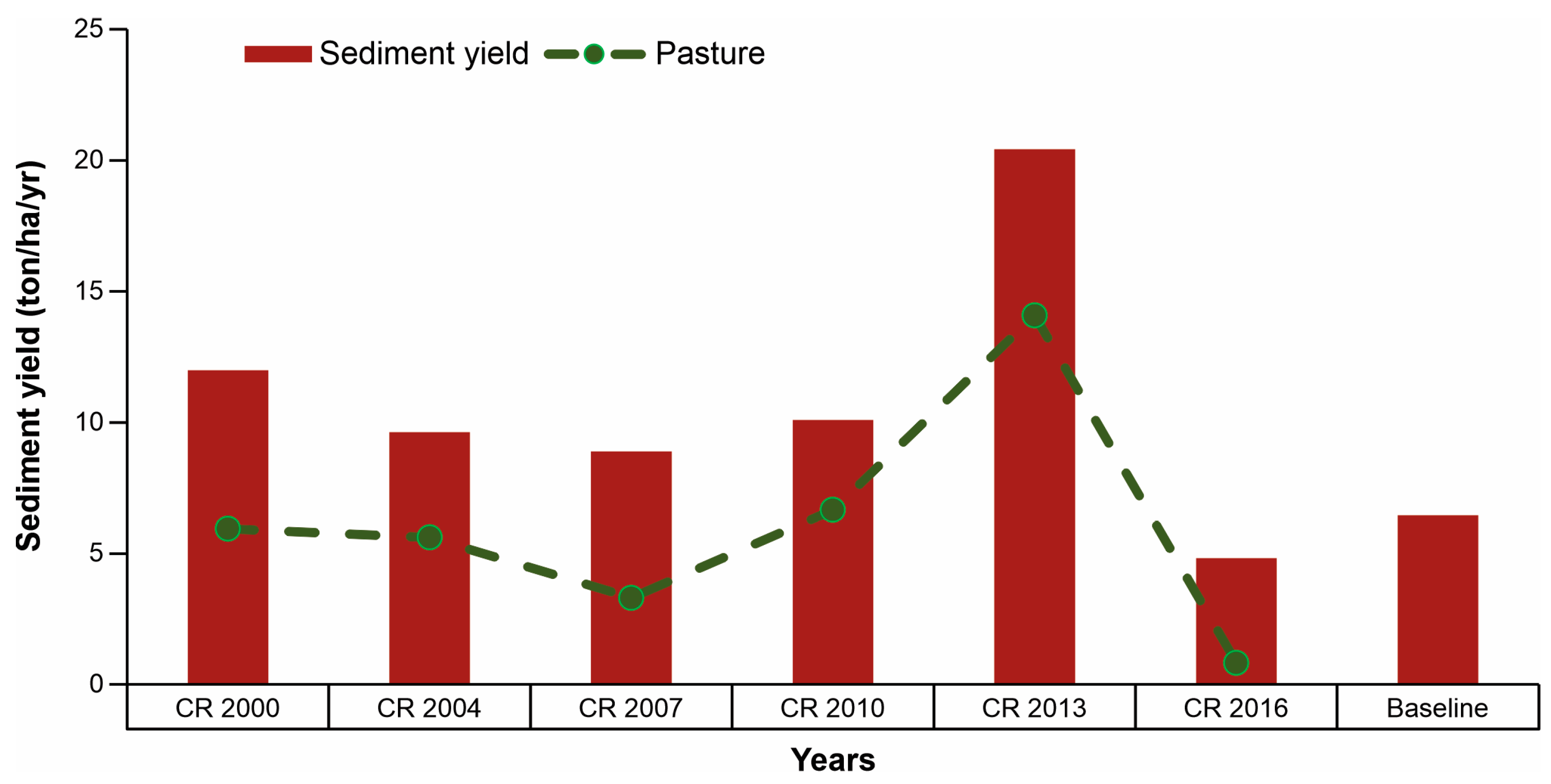
| LULC | ET (mm) | SURFQ (mm) | GWQ (mm) | SYLD (ton/ha) |
|---|---|---|---|---|
| Land use 2000 | 679.10 | 381.23 | 639.79 | 12.00 |
| Land use 2004 | 688.40 | 387.58 | 626.03 | 9.63 |
| Land use 2007 | 689.80 | 386.94 | 625.00 | 8.90 |
| Land use 2010 | 688.80 | 377.40 | 631.82 | 10.10 |
| Land use 2013 | 686.40 | 376.57 | 633.41 | 20.42 |
| Land use 2016 | 689.10 | 398.87 | 611.20 | 4.83 |
| Baseline | 670.7 | 340.6 | 681.47 | 6.47 |
Disclaimer/Publisher’s Note: The statements, opinions and data contained in all publications are solely those of the individual author(s) and contributor(s) and not of MDPI and/or the editor(s). MDPI and/or the editor(s) disclaim responsibility for any injury to people or property resulting from any ideas, methods, instructions or products referred to in the content. |
© 2023 by the authors. Licensee MDPI, Basel, Switzerland. This article is an open access article distributed under the terms and conditions of the Creative Commons Attribution (CC BY) license (https://creativecommons.org/licenses/by/4.0/).
Share and Cite
Viana, J.F.d.S.; Montenegro, S.M.G.L.; Srinivasan, R.; Santos, C.A.G.; Mishra, M.; Kalumba, A.M.; da Silva, R.M. Land Use and Land Cover Trends and Their Impact on Streamflow and Sediment Yield in a Humid Basin of Brazil’s Atlantic Forest Biome. Diversity 2023, 15, 1220. https://doi.org/10.3390/d15121220
Viana JFdS, Montenegro SMGL, Srinivasan R, Santos CAG, Mishra M, Kalumba AM, da Silva RM. Land Use and Land Cover Trends and Their Impact on Streamflow and Sediment Yield in a Humid Basin of Brazil’s Atlantic Forest Biome. Diversity. 2023; 15(12):1220. https://doi.org/10.3390/d15121220
Chicago/Turabian StyleViana, Jussara Freire de Souza, Suzana Maria Gico Lima Montenegro, Raghavan Srinivasan, Celso Augusto Guimarães Santos, Manoranjan Mishra, Ahmed Mukalazi Kalumba, and Richarde Marques da Silva. 2023. "Land Use and Land Cover Trends and Their Impact on Streamflow and Sediment Yield in a Humid Basin of Brazil’s Atlantic Forest Biome" Diversity 15, no. 12: 1220. https://doi.org/10.3390/d15121220
APA StyleViana, J. F. d. S., Montenegro, S. M. G. L., Srinivasan, R., Santos, C. A. G., Mishra, M., Kalumba, A. M., & da Silva, R. M. (2023). Land Use and Land Cover Trends and Their Impact on Streamflow and Sediment Yield in a Humid Basin of Brazil’s Atlantic Forest Biome. Diversity, 15(12), 1220. https://doi.org/10.3390/d15121220