Abstract
Nuclear magnetic resonance (NMR) spectroscopy is an innovative method for wine analysis. Every grapevine variety has a unique structural formula, which can be considered as the genetic fingerprint of the plant. This specificity appears in the composition of the final product (wine). In the present study, the originality of Hungarian wines was investigated with 1H NMR-spectroscopy considering 861 wine samples of four varieties (Cabernet Sauvignon, Blaufränkisch, Merlot, and Pinot Noir) that were collected from two wine regions (Villány, Eger) in 2015 and 2016. The aim of our analysis was to classify these varieties and region and to select the most important traits from the observed 22 ones (alcohols, sugars, acids, decomposition products, biogene amines, polyphenols, fermentation compounds, etc.) in order to detect their effect in the identification. From the tested four classification methods—linear discriminant analysis (LDA), neural networks (NN), support vector machines (SVM), and random forest (RF)—the last two were the most successful according to their accuracy. Based on 1000 runs for each, we report the classification results and show that NMR analysis completed with machine learning methods such as SVM or RF might be a successfully applicable approach for wine identification.
1. Introduction
Nuclear magnetic resonance (NMR) spectroscopy is a structure analysis method applied since the 1940s. The NMR technique provides several advantages, including easy sample preparation and short running time [1]. This is an easy and rapid way to obtain the chemical composition of grapes, grape juice, must, and wine; moreover, it is also suitable for the identification of small organic compounds (metabolite profiling), such as amino acids [2], organic acids, alcohols [3,4], sugars, and phenolic compounds [5]. Thus, in recent years, NMR spectroscopy has found increased application in food science and agriculture, including the quality control [6], authentication [7], and analysis of an immense variety of food products [8,9,10].
The principle behind NMR spectroscopy is that certain nuclei have magnetic moments. The practice of this technique applies electromagnetic radiation for the selective excitation of these nuclei with magnetic moments. The excitation is followed by a detectable relaxation. Information can be obtained by the detection of the relaxation after excitation for different pulse lengths and pulse series. Data about the density of the nuclei and the surrounding electrons in the substance, such as information on neighboring connections, can also be collected [11]. This technique can be applied to study the chemical relations in substances. The spectrum provides information about the number and shading of atoms in molecules and about the number and type of neighboring atoms around a certain nucleus. In the name NMR, ‘magnetic’ refers to the fact that the physical phenomenon occurs only in a strong magnetic field, hence the investigated solution or solid sample is placed within the magnet and surrounded by a superconducting coil. Liquid helium (LHe) is used as the coolant for superconducting magnets or samples tested in a high magnetic field.
Only those nuclei with an odd number of protons and/or neutrons can be detected by NMR spectroscopy. These are called active nuclei. There are two types of NMR spectroscopy: high resolution and broad spectrum. High resolution spectroscopy shows sharp signals, which primarily provide data about the molecular configuration. Broad spectrum spectroscopy provides information about the material structure and the physical interactions in a solid state.
Most NMR-based metabolomics studies use proton 1H-NMR spectroscopy because 1H-atoms occur in almost every organic compound and known metabolite [12]. Single dimensional 1H-NMR spectra are especially useful in metabolomics studies because the technique is well automated, highly dependable, and very fast.
NMR spectroscopy at 400 MHz is an innovative technique in wine analysis. It provides a unique spectroscopic fingerprint of every sample that contains all the information concerning variety, geographical origin, vintage, physiological state, and technological treatments, among other features [13]. The extreme sensitivity of the instrument allows the determination of 53 chemical parameters from milligrams of samples.
One 1H-NMR-spectrum contains the chemical information of the sample, which is sufficient to identify and quantify 50–100 metabolites simultaneously [14,15]. The identification process is supported by a high number of references that were produced from the 1H-NMR spectra of well-known metabolites and are available in open-access databases.
With this method, 53 wine components can be measured simultaneously and quickly, and a complex dataset is created that is suitable for a follow-up multivariate statistical analysis with the aim of determining the geographical origin and/or the variety of the wine. Among the studied 53 components, the most important eight parameters of the wine analysis are the following: alcohol, glucose, fructose, glycerol, tartaric acid, lactic acid, total extract, and sugar-free extract. In addition to these basic parameters, decomposition products, such as acetic acid, acetoin, biogene amines (ethyl-acetate), and polyphenols (caftaric acid, gallic acid, shikimic acid, and trigonelline) can be determined; moreover, the marker compounds of fermentation (2,3-butanediol, 2-phenylethanol, 3-methyl-butanol, acetaldehyde, galacturonic acid, methanol, and succinic acid) are also detectable.
The complete NMR spectrum of the wine sample can be considered as a molecular fingerprint; hence it can be directly used to compare and identify wines. This chemical/spectroscopical information works as the wine metabolome, which is modified by several wine-making factors, such as viticulture technique, pedoclimate [16], grapevine variety, fermentation technique, and geographical origin [17,18,19,20].
Magda et al. [21] reported that wine classification had been carried out in four spectral fields. It was proven that in the most discriminative spectral field (5.1–9.8 ppm), 100% of the samples could be distinguished based on the geographical origin and variety.
NMR-based wine profiling uniquely combines the examinations for quality control, quality assurance and authentication; therefore, NMR spectroscopy is a daily routine for industrial quality assurance and technological control.
In this study, Hungarian wine samples were analyzed by 1H-NMR spectroscopy in order to distinguish four varieties and their geographical origin. Data were analyzed by four classification methods (linear discriminant analysis (LDA), neural networks (NN), support vector machines (SVM), and random forest (RF)) from which SVM and RF were the most successful based on their classification accuracy regarding the variety and geographical origin.
2. Materials and Methods
2.1. Samples
Wine samples of four varieties (Cabernet Sauvignon, Blaufränkisch, Merlot, and Pinot Noir) were analyzed. For better comparability, samples of two vintages from two wine regions (Eger: 47.9045° N, 20.3384° E, Villány: 45.86951° N 18.45562° E) were collected. The samples used for the measurements were obtained from different wineries. They were samples direct from winery casks. The number of samples with their varieties, as well as the place and year of their origin are summarized in Table 1.

Table 1.
The number of samples involved in the study of varieties Cabernet Sauvignon, Blaufränkisch, Merlot, and Pinot Noir from Hungarian wine regions Villány and Eger and vintages 2015 and 2016. The total sample size was 861.
2.2. Apparatus and Measurement
The first step in the measurement method is sample preparation. This step is necessary because the pH of wine has a relatively wide range, usually between pH 2.9 and pH 3.7. However, for measurement, we need a stable pH of 3.10 +/− 0.04 for each sample. In addition, the internal calibration standard material, the TSP, and the reference deuterated compound, D2O, are added during sample preparation, without which it would be impossible to perform the NMR assay. Thus, the first step in the sample preparation process was to adjust the pH to the target value (pH 3.10 +/− 0.04). A volume of 900 µL of the sample to be measured was then transferred into a 2 mL cryogenic sample tube using an automatic pipette and placed into the shaker of the titration unit BTpH (Bruker Biospin, Rheinstetten, Germany). The electrode of the instrument was inserted into the sample tube, ensuring contact with the sample, and then titration was started. The instrument first measured the pH of the wine sample and then added 100 µL of phosphate buffer containing 1 M KH2PO4, TSP, and D2O, and NaN3. Depending on the pH measured, acid (HCl) or alkali (NaOH) was added to the sample until the pH reached the target value.
During titration, the sample was shaken continuously to homogenize it as much as possible.
Adjusting the pH to a target value is particularly important because even a very small pH difference of about 0.05 units between samples can significantly alter the chemical shift of the NMR spectra. Thus, this process greatly contributes to the NMR spectra obtained during the measurement.
A volume of 600 µL of the titrated sample was then pipetted into a 5 mm diameter NMR tube, and the spinner and the barcode for identification were applied to this tube at a specified height. Finally, the sample was inserted into the automatic sample changer of the NMR instrument.
NMR measurements were carried out with a Bruker 400-MHz AVANCE III HD NanoBay spectrometer (Bruker Biospin, Rheinstetten, Germany) equipped with a 5-mm BBO (broadband observe) probe with Z-gradient coil. The 400 in the name of the device refers to the 400 MHz magnet. A Bruker automatic sample changer Sample Xpress (Bruker Biospin, Rheinstetten, Germany) was applied. We included a waiting period of 5 min for temperature equilibration prior to every measurement. Each 1H NMR spectrum was gathered at 290 K using a standard Bruker pulse program “zgpr30” completed with a relaxation delay (D1) of 3 s and an acquisition time of 11 s. The total data points were set to 131,072; 128 scans and two dummy scans were gathered with a spectral width of 15.0191 ppm (6009.615 Hz) and a receiver gain of 44. The total measurement time resulted in 30 min per sample. The raw Free Induction Decay dataset (FID) was multiplied with a Gaussian window function, then every spectrum was automatically phased and baseline corrected. The NMR spectra were analyzed using Bruker’s chemical component analysis package “Wine-Profiling (TM) 3.0”. Spectra were acquired under an automation procedure (automatic shimming and automatic sample loading), so the obtained NMR spectrum is the end product of a fully automated process, which we are able to open and evaluate in software called TopSpin version 3.2 and AMIX with version number 3.9.15 (Bruker Biospin, Rheinstetten, Germany). The data we can see in the NMR report were generated by the software. In addition to the principle parameters, five compounds were identified and measured in each wine spectrum: caftaric acid, epicatechin, gallic acid, shikimic acid, and trigonelline.
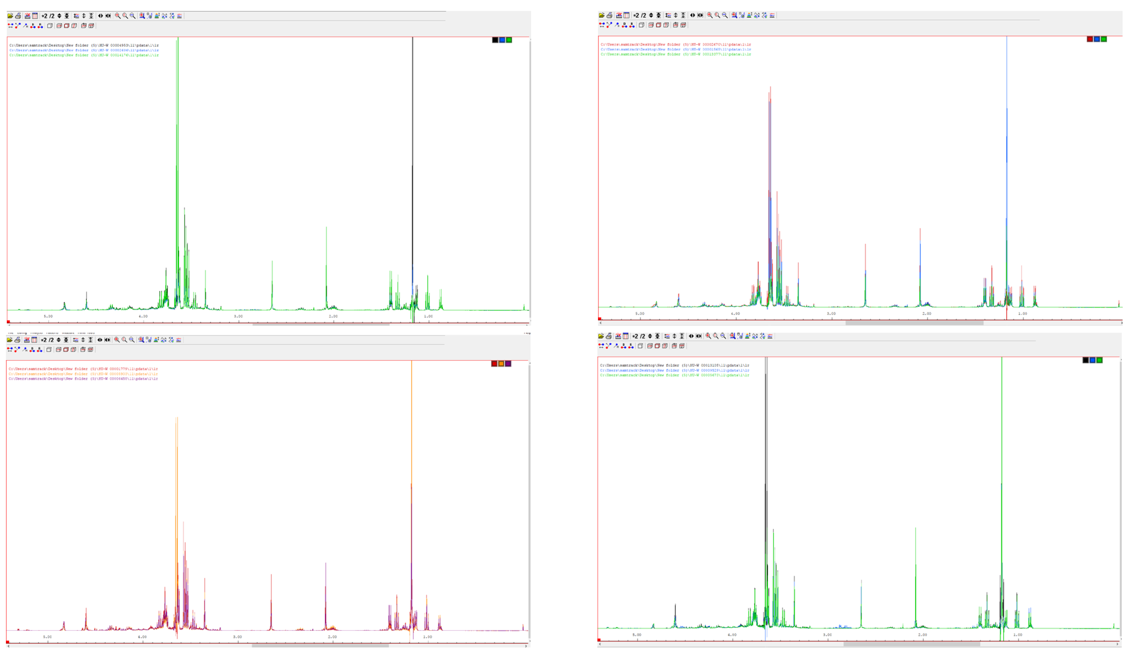
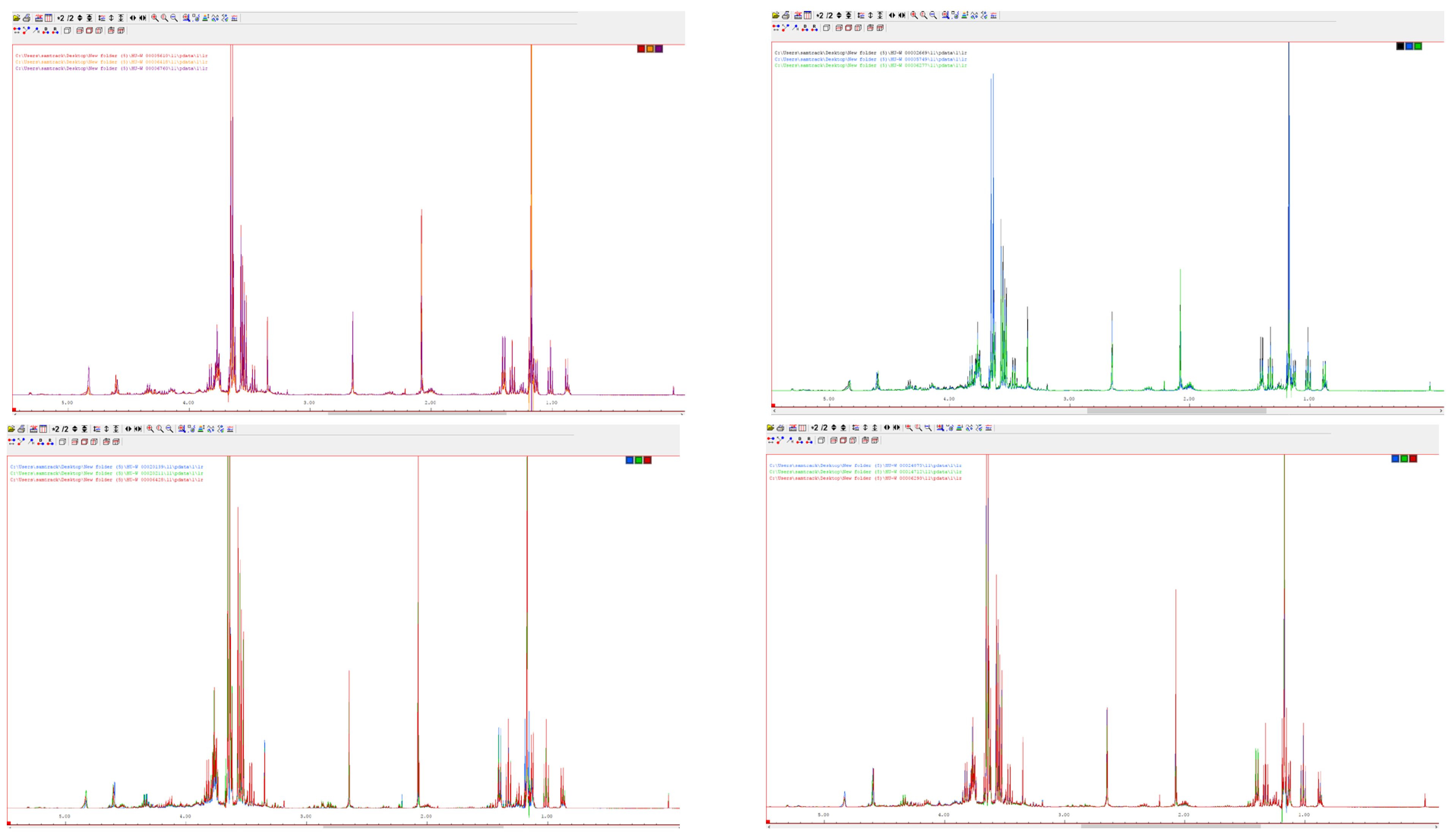
The following spectra show the changes in the intensity of the key resonances in the four varieties and the two wine regions (Figure 1).
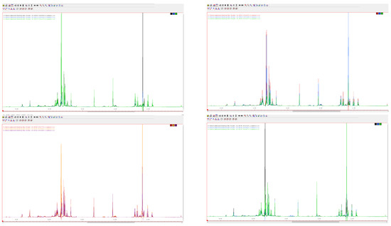

Figure 1.
The spectra of the varieties Cabernet Sauvignon (C, first row), Blaufränkisch (B, second row), Merlot (M, third row), and Pinot Noir (P, fourth row) with origin Eger (E, left) and Villány (V, right) from 2015. The plots show spectra of three samples between 3.00 and 4.00 ppm. (Source: own screenshots)
2.3. Classification Methods
Based on a thorough study of literature, Amargianitaki et al. [22], Masetti et al. [23], and recently Kalogiouri and Samanidou [24] introduced and compared several kinds of multivariate analysis methods (PCA, PLS-DA, kNN, NN, SIMCA, and SVM) to investigate their classification success depending on cultivar, vintage, geographical origin, and even seasonality, while considering NMR data. In this paper, we applied four classification methods (LDA, NN, RF, and SVM) and investigated their success in variety and origin classification.
As we had previous classification knowledge about the 22-trait dataset (i.e., origin and variety), we tested four supervised machine learning classification methods to separate the four varieties from two origins (eight groups altogether). For this, we randomly split our dataset into two parts, the training subset and the test subset, using a 3:1 ratio. The eight groups had quite different sample sizes; therefore, the two subsets were created so they kept the original sample size ratios. In this way, we could avoid to have such training/test sets that do not contain (or contain too few) samples from the smallest groups (Merlot from Villány, 2016 or Blaufränkisch from Eger, 2015). For all four methods, we performed 1000 runs with different random subsets. The classification result produced by the training set was then tested for the remaining test dataset.
2.3.1. Linear Discriminant Analysis (LDA)
LDA as a linear model has much in common with the widely used MANOVA, although their goals and interpretation are different. MANOVA indicates whether the mean differences across the groups are significant on an optimized linear combination of the original traits (), whereas LDA searches hyperplanes () of the traits that can separate the preliminary groups as much as possible. The preliminary grouping factor is an explaining factor in case of MANOVA, whereas it is the dependent variable for LDA. In our analysis, we applied multiclass LDA [25]. From the s, we used the lowest number ones that were significant and had the appropriate effect of classification. Limitations of LDA are that it is quite sensitive to outliers and unequal sample sizes, as was our case. It also requires multivariate normality, which is often violated (as in our case, too), although it is quite robust to this as well as to the dispersion homogeneity violation when all the other assumptions more or less hold true. Multicollinearity can also cause biased results due to highly redundant traits [25,26].
2.3.2. Neural Networks (NN)
NN are a set of supervised machine learning algorithms modelling human brain recognition and response. The methods are widely used, amongst several others, for classification. Through the training, a model is created that provides the inputs with weights, summarizes the gained information by one or more functions, and defines an activation function that calculates the output. With an increasing number of layers, the algorithms become more and more complex and the number of calculations increases drastically [22,23,24].
2.3.3. Random Forest
Based on the classification and regression tree (CART), RF makes its classification decision by a consensus (the most common output), according to a large number of trees (ntree) with individual predictions. The main point of the method is that for the development of each tree, a random sample from the whole training dataset is taken with replacement. The dataset that is not used in a step (approximately 1/3) is called out-of-bag (OOB). The algorithm randomly uses a subset of traits of size mtry. A great advantage of RF is that it is not sensitive to outliers and missing data [26,27,28,29].
2.3.4. Support Vector Machines (SVM)
The main goal of SVM is to define a hyperplane in n-dimensional space that distinctly classifies the data points by maximizing the distances between the points of different groups. It is a very powerful method that can be successful even if the spatial distribution of the groups is quite complex, as several different types of kernel functions can be applied for SVM [26,30].
2.4. Model Evaluations
To measure the classification quality of the models with respect to the test dataset, we used the following measures: percent of records correctly classified (accuracy), true positive classification rate (sensitivity or recall ), true negative classification rate (specificity), balanced accuracy (average of sensitivity and specificity), positive prediction value (precision, ), negative prediction value, prevalence, detection rate, detection prevalence [31], and the area under the receiver operating character (ROC) curve (AUC) [32,33]. Based on Powers [34], the score was defined as The rate of agreement between observed and predicted classifications was measured by Cohen’s Kappa [35].
For the case of the RF model, the error rate of the tree if it is applied to the OOB data (OOB error) was also calculated. We optimized the RF parameters by tuning mtry and ntree with respect to the OOB error estimate and root mean square error (RMSE), considering other classification quality measurements, such as accuracy, F1 score, and AUC, and finally set them to ntree = 500 and mtry = 4. As a splitting rule, we applied the mean decrease in accuracy and the mean decrease in the Gini Index [36].
For the case of the SVM model, radial basis function was chosen. Again, optimization of the parameters was subjected to a tuning process that resulted in a gamma value of 0.05 and a cost value of 10.
For the case of RF, we calculated the variable importance based on the overall mean decrease in accuracy (overall MDA) and MDA by categories [37,38,39]. For this, we used the OOB sample set to calculate accuracy. The values of a specific feature were then randomly shuffled, while all other feature values remained the same, and the accuracy of the shuffled data was calculated. Finally, we took the difference between these two accuracy values and their mean across all trees (MDA). This importance measure is the overall MDA, but when breaking them down by outcome categories, MDA can also be provided for each category. For the case of the SVM model, variable importance was calculated based on the AUC of the ROC curve. Note that these methods provide no information on whether a variable is important as a main effect or as part of an interaction.
Model development was conducted in R 4.0.3 [40] with packages ‘randomForest’ [41,42], ‘caTools’ [43], ‘e1071’ [44], ‘caret’ [45], and MASS [46] to perform LDA, NN, SVM, and RF models. Figures were produced using the package ‘ggplot2’ [47] and ROCR [48].
2.5. Visualization
To visualize the differences between the varieties and wine regions considering some components that were selected as having the highest classification power, we calculated the (x-min(x))/(max(x)-min(x)) transformation that makes all of the components comparable independently from their magnitudes. With this transformation, the highest values get the rate of 1 and the lowest the rate of zero. In a spider web we can recognize which variety/wine region resulted in “high” or “low” values of the most discriminating components.
3. Results
3.1. Linear Discriminant Analysis and Neural Networks
As a data preparation, we center-scaled the 22 traits that were involved in the analysis. Mahalanobis distances were calculated and the multivariate outliers were detected. The traits were tested against normality and their Pearson’s correlation was calculated. We could see that both normality and variance homogeneity assumptions were violated at a moderate rate. Despite this, LDA performed quite well: the percentage separation achieved by the first three discriminant functions (DV1, DV2, DV3) were 42, 26, and 17% with canonical correlations all over 0.75 and with all Wilk’s lambda values being significant. Compared to the other methods, LDA was the weakest model in separating the eight groups (four varieties and two wine regions).
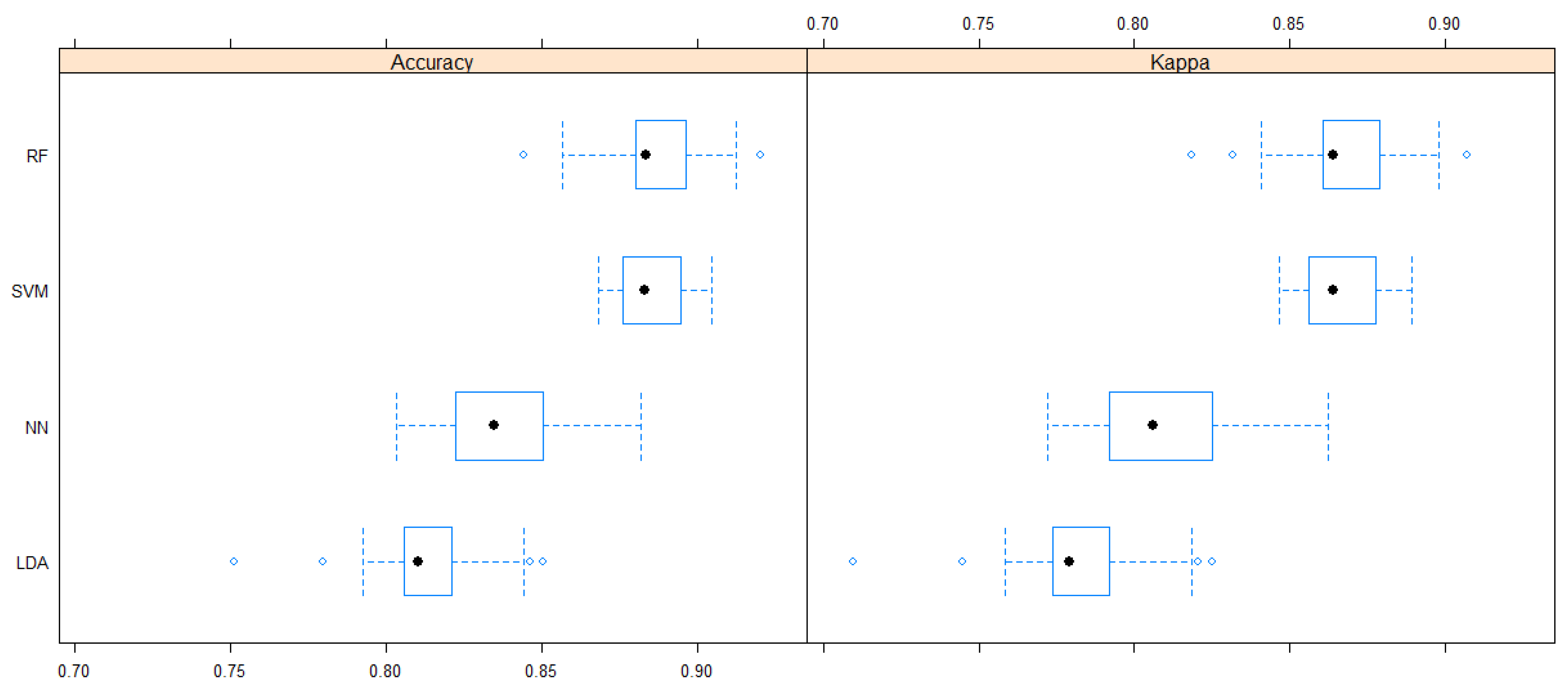
A NN model was developed by 100 iterations with bootstrap resampling of 25 replications to tune the hyper-parameters. The number of units in the hidden layer was 5, and the regularization parameter was 0.1. The NN models worked better than LDA models, though notably worse than RF or SVM models. Based on 1000 runs of each method, according to model accuracy and Cohen’s Kappa, we have chosen RF and SVM models to evaluate them in detail (Figure 2).
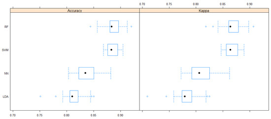
Figure 2.
Comparison of classification power of four methods, i.e., linear discriminant analysis (LDA), neural networks (NN), support vector machines (SVM), and random forest (RF) expressed by their accuracy and Cohen’s Kappa based on 1000 runs of each method. The aim was to separate the varieties (Cabernet Sauvignon, Blaufränkisch, Merlot, and Pinot Noir) and wine regions (Eger, Villány) considering their 22 traits of alcohols, sugars, acids, decomposition products, biogene amines, polyphenols, and fermentation compounds based on 861 samples from 2015 and 2016. Black symbols are for the median values.
3.2. Random Forest (RF) and Support Vector Machines (SVM)
The ratio of accuracy calculated for the test and training dataset was as high as 0.99 and 0.94 in case of RF and SVM, respectively, which confirmed that overfitting did not bias our results (Table 2 and Table 3).
Table 2.
Random forest classification quality of different variables calculated for the dependent variable ‘variety and origin’ (CE, CV, BE, BV, ME, MV, PE, PV *). TP: true positive; TN: true negative; FP: false positive; FN: false negative; N = total number of observations; AUC: area under the ROC curve; ROC: receiver operating character; CI: 95% confidence interval; OOB: out-of-bag.
Table 3.
Support vector machine (SVM) classification quality of different variables calculated for the dependent variable ‘variety and origin’ (CE, CV, BE, BV, ME, MV, PE, PV *). TP: true positive; TN: true negative; FP: false positive; FN: false negative; N = total number of observations; AUC: area under the ROC curve; ROC: receiver operating character; CI: 95% confidence interval; OOB: out-of-bag.
The overall accuracy of the RF and SVM models applied to the test dataset were as high as 0.95 and 0.94, respectively. Based on the sensitivity, precision, balanced accuracy, and AUC values, both RF and SVM models most successfully predicted the categories of Pinot Noir from Eger and Villány and Blaufränkisch from Villány. The sensitivity values of these groups were 100% for RF and higher that 91% for SVM. All three groups exceeded 0.92 or 0.87 precision, 0.98 or 0.94 balanced accuracy, 0.99 or 0.98 AUC, and 0.96 or 0.89 F1 score for RF and SVM, respectively.
The prediction of Blaufränkisch from Eger was the poorest, which was not surprising, as we had quite a low number of observations in this group (9 and 17 in the two years). The sensitivity of this category was as low as 0.50 and 0.67 for RF and SVM, respectively, together with low precision (0.60 and 0.57) and F1 values (0.55 and 0.62). Balanced accuracy (0.73 and 0.81) and AUC (0.93 and 0.73) values were also the lowest for this group.
Therefore, we can conclude that the most effective method of classification was RF followed by SVM, both with highly significant weighted Kappa (0.95, p < 0.001), and even RF was unreliable when the number of observations was very low.
4. Discussion
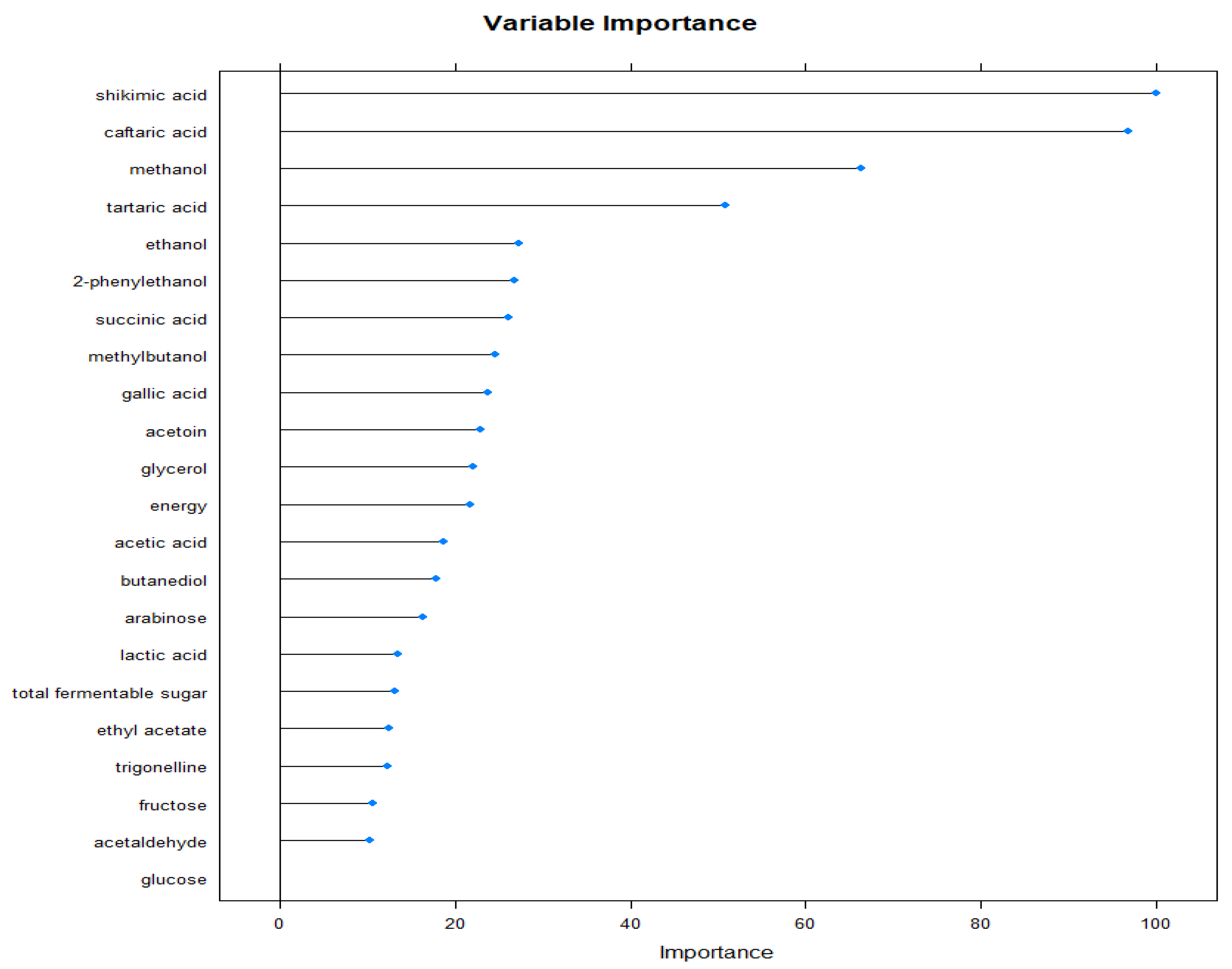
We calculated the variable importance based on the SVM and RF model outputs, whereas the varieties Cabernet Sauvignon, Blaufränkisch, Merlot, and Pinot Noir and wine regions Eger and Villány were classified considering their 22 traits of alcohols, sugars, acids, decomposition products, biogene amines, polyphenols, and fermentation compounds based on 861 samples from 2015 and 2016. The first seven most important variables were the same in both the SVM and RF models (Figure 3).
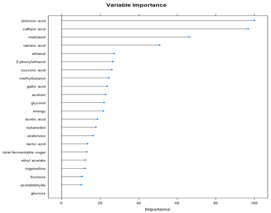
Figure 3.
Variable importance calculated by the SVM method when performing classification of the varieties (Cabernet Sauvignon, Blaufränkisch, Merlot, and Pinot Noir) and wine regions (Eger, Villány) considering their 22 traits of alcohols, sugars, acids, decomposition products, biogene amines, polyphenols, and fermentation compounds based on 861 samples from 2015 and 2016. Note that the first seven most important variables were the same in both the SVM and RF models.
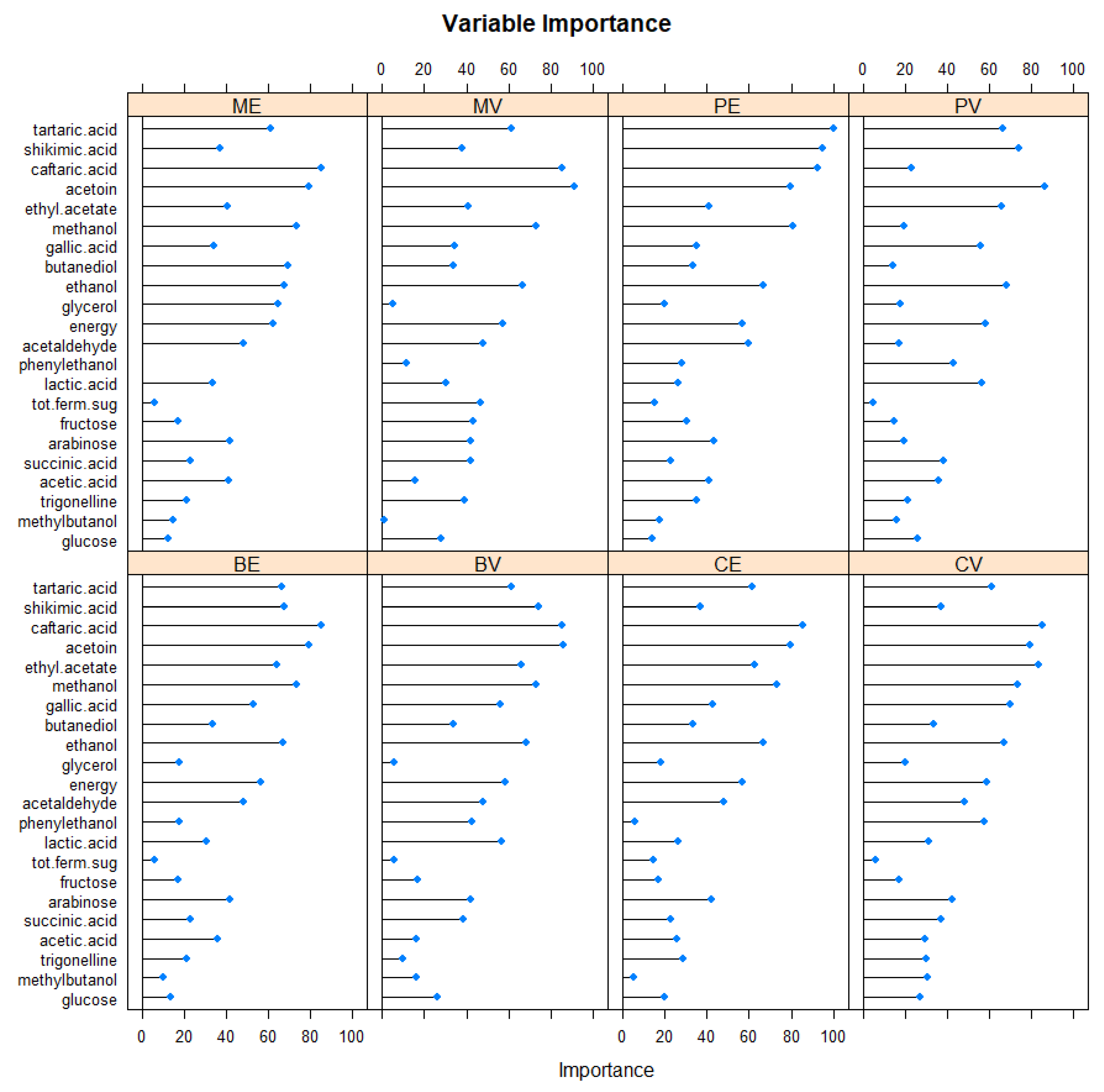
The variable importance values were also calculated group by group (Figure 4).
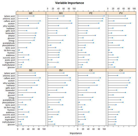
Figure 4.
Variable importance calculated for all variety/wine region groups using the SVM method when performing classification of the varieties (Cabernet Sauvignon (C), Blaufränkisch (B), Merlot (M), and Pinot Noir (P)) and wine regions (Eger (E), Villány (V)) considering their 22 traits of alcohols, sugars, acids, decomposition products, biogene amines, polyphenols, and fermentation compounds based on 861 samples from 2015 and 2016 (e.g., CE: Cabernet Sauvignon grown in Eger).
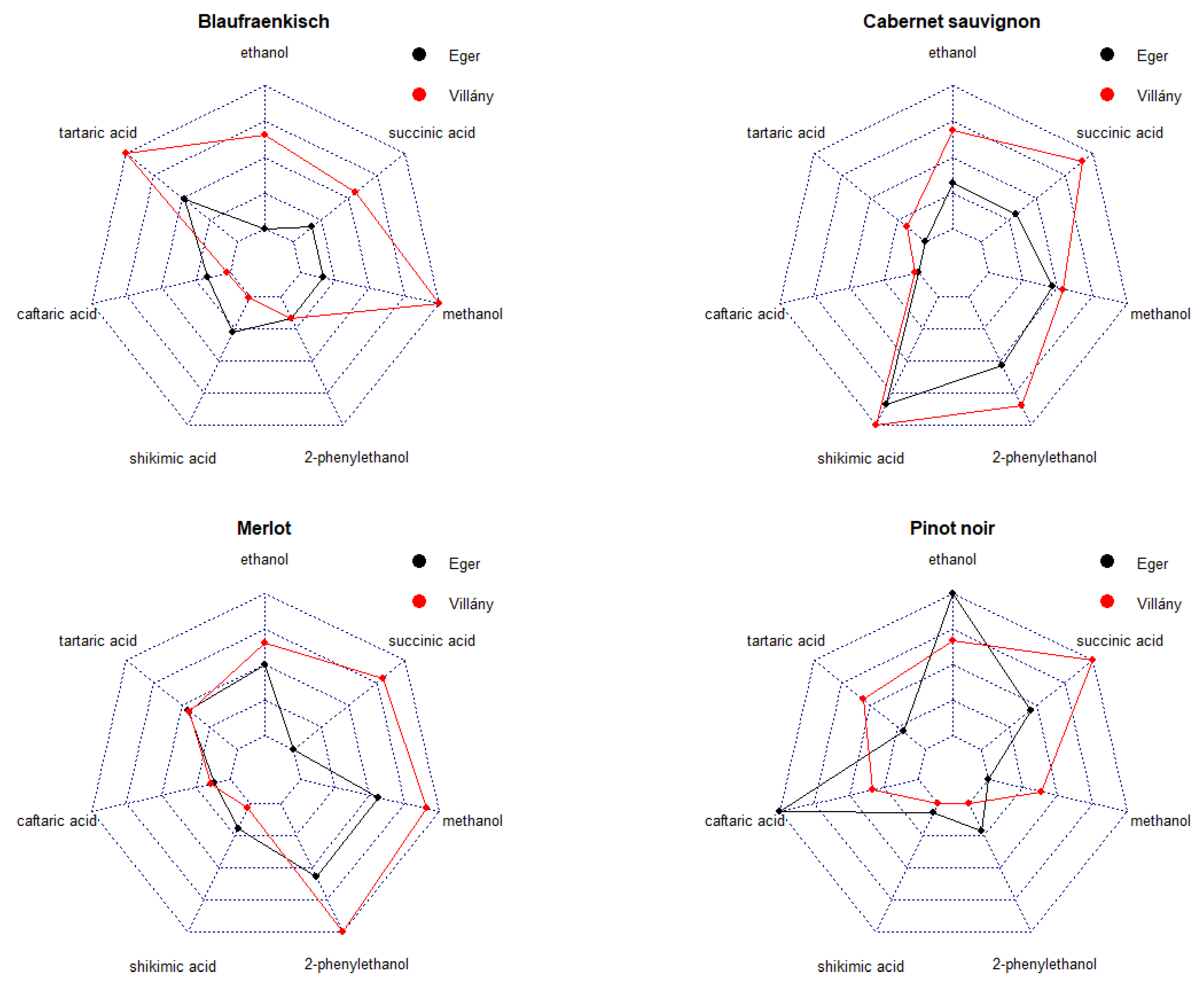
Finally, to support the discussion, we visualized the variety/wine region characteristics based on the seven most important variables (shikimic acid, caftaric acid, methanol, tartaric acid, ethanol, 2-phenilethanol, and succinic acid). To make the variables of different magnitudes and units comparable, we calculated (x-min(x))/(max(x)-min(x)). This transformation shifts the minimum value to zero and the maximum value to 1 and all the other values are shifted in the (0,1) interval proportionally to their magnitudes. In this way, we can recognize the main differences in wine samples as having proportionally ‘great’ or ‘small’ values from the different compounds (Figure 5).
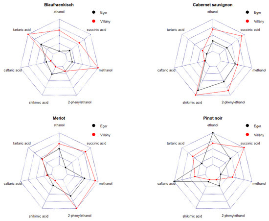
Figure 5.
The characteristics of the varieties (Cabernet Sauvignon, Blaufränkisch, Merlot, and Pinot Noir) and wine regions (Eger, Villány) considering their seven components that were selected as having the highest classification effects (ethanol, tartaric acid, methanol, 2-phenylethanol, succinic acid, caftaric acid, and shikimic acid) based on RF and SVM models. The original values were transformed to the (0,1) interval keeping their proportion to make them unitless comparable.
RF and SVM models agreed that the seven overall most important parameters were shikimic acid, caftaric acid, methanol, tartaric acid, ethanol, 2-phenylethanol, and succinic acid. Ethanol, methanol, and succinic acid refer to alcoholic fermentation, whereas caftaric acid, shikimic acid, and tartaric acid are components characteristic for grapes. The parameter 2-phenylethanol is an indicator of both the intensity of fermentation and the condition of the grapes in the flavor of the grape skin.
According to Figure 4 and Figure 5, out of the selected seven parameters, 2-phenylethanol, methanol, and succinic acid are the main parameters that can be used to differentiate between the two wine regions (Eger and Villány) in the cases of Cabernet Sauvignon and Merlot. In samples from Villány, these parameters were definitely higher than in those from Eger. Succinic acid and methanol together with tartaric acid have strong power in classification in Blaufränkisch and Pinot Noir that can differentiate wine region with their high values in Villány samples. Higher ethanol and caftaric acid were more characteristic for the Pinot Noir from the Eger wine region.
High shikimic acid and 2-phenylethanol were characteristic for Cabernet Sauvignon, high ethanol for Pinot Noir; and high 2-phenylethanol for Merlot.
Each grape variety has a unique structural formula that is typical for its genetic map: this is called the “fingerprint” of the plant. This species specificity is reflected in the composition of the finished product (wine) made from it. That is why analytical chemistry is playing an increasingly important role in winemaking.
Classification of wine samples according to variety, geographical region, vintage, or even seasonality [49] based on 1H NMR metabolomics data is an intensively investigated topic. Anastasiadi et al. [5] classified Greek wines according to variety, region, and vintage by using 1H NMR metabonomic data and the PCA method and proved that their classification results were less successful based on HPLC data. As for the data analysis, several multivariate methods such as MANOVA [20,50,51,52], cluster analysis [19], principal component analysis (PCA) [19,20,22,49,50,51,53,54], partial least square discriminant analysis (PLS-DA) [3,48,49,52,53,55,56,57,58], orthogonal projections to latent structures (OPLS) [59], linear or quadratic discriminant analysis (LDA/QDA) [20,22,52,60], and soft independent modeling of class analogy (SIMCA) [60] are used. Monakhova et al. [56] improved their discriminant analysis results introducing the PCA method combined with independent components analysis with an NMR fingerprinting case study of German wines.
Machine learning classification methods widely used in food sciences, such as neural networks (NN), random forest (RF), and support vector machines (SVM), are quite rarely used for wine sample differentiation, although they are very effective models. One advantage of RF and SVM over other classification methods is that they are less susceptible to overfitting. SVM works well even with moderately low sample sizes compared to the number of the measured variables, although it is less successful for a large dataset. These advantages were our main motivation to compare LDA, NN, RF, and SVM methods. We found RF and SVM models as most effective based on our 1H NMR metabonomic data of four varieties from two regions, which is in agreement with Martelo-Vidal and Vázquez [60], who compared three methods (SIMCA, LDA, and SVM) to classify 39 red wines of two origins of Spain and found the SVM method as the most efficient based on their polyphenolic profiles.
Mascellani et al. [50] investigated Czech wine samples of different types, varieties, and geographic origin. They applied PCA, hierarchical clustering, PLS-DA, and RF methods with different goals of classification. The most successful RF models were trained for the classification of 13 wine grape varieties in three steps based on 1H NMR spectroscopy. In the first step, they classified different wine types; in the second step, different varieties were discriminated; and in the third step, the discrimination of Chardonnay from Pinot Noir wines was addressed. As for the variety classification success (without geographical region classification), they got results for Pinot Noir (96%), Blaufränkisch (96%), and Cabernet Sauvignon (77%) that are in accordance with our RF results (Pinot Noir (0.99% and 100%), Blaufränkisch (98%, 100%), Cabernet Sauvignon (98% and 99%) for Eger and Villány, respectively). The most important features were detected as proline, phenylalanine, methanol, catechin, tyrosine, and epicatechin, from which our models agreed in the case of methanol and catechin. Viggiani et al. [57] also found succinic acid, proline, and 2,3-butanediol as the most discriminating contents in wine samples when they separated them according to vintage and geographical region.
Different wine varieties produced in Germany were analyzed by Godelmann et al. [13] using 1H NMR spectroscopy. They applied multivariate data analysis (PCA, LDA, and MANOVA). Pinot Noir was again among the successfully classified varieties resulting in shikimic acid, caftaric acid, and 2,3-butanediol as having the strongest classification power. The classification was performed regarding grape variety, year of vintage, and geographical origin. The results of Papotti et al. [55] correspond to these findings as they also found 2,3-butanediol, lactic and succinic acids, threonine, and malic acid as the most important compounds in their PCA- and PLS-DA-based classification of varieties.
According to Geana et al. [52], among other varieties, Cabernet Sauvignon, Merlot, and Pinot Noir wines, produced in Romania, were also successfully discriminated using NMR-based metabolomics with MANOVA and LDA data analysis. Shikimic, lactic, acetic, citric, and succinic acids were detected as the most significant variables in the classification of varieties. Based on 6-year data, vintages were also classified successfully. However, Magda et al. [21] reported that using PCA and LDA methods, they were unable to differentiate five vintages. Similarly, Caruso et al. [53] found that their two vintages were also not differentiable groups based on their PCA-, LSD-, or PLS-DA-based approach.
5. Conclusions
We can conclude that the 1H NMR-based metabolomics completed with random forest or support vector machines method are promising approaches for classification of Cabernet Sauvignon, Blaufränkisch, Merlot, and Pinot Noir wine samples according to their variety and region. Beyond the high level correct classification rate, these methods have the advantage that we can select the most important traits that have notable effects on separation. In our case study, shikimic acid, caftaric acid, methanol, tartaric acid, ethanol, 2-phenilethanol, and succinic acid were the most important traits. Moreover, the LDA and NN methods performed less successful classification results.
The differences between the two geographical regions in the chemical profiles of the vines can be caused by the undoubtedly different climate conditions: in Eger, the mean annual temperature is about 10.5 °C, in Villány it is 11.5 °C. The mean number of sunny hours in Eger is 1990 and it is almost a Mediterranean value, more than 2100 in Villány. The growing season in Eger is longer, grapes are usually harvested in November, 2–3 weeks later than in Villány.
Author Contributions
Conceptualization, Á.D.N.S.; data curation, M.L.; formal analysis, M.L.; investigation, Á.P.S. and R.M.; methodology, Á.D.N.S. and M.L.; software, M.L.; validation, M.L.; visualization, M.L.; writing—original draft, M.L. and Z.V.; writing—review and editing, M.L. All authors have read and agreed to the published version of the manuscript.
Funding
This research received no external funding.
Institutional Review Board Statement
Not applicable.
Informed Consent Statement
Not applicable.
Data Availability Statement
Not applicable.
Conflicts of Interest
The authors declare no conflict of interest.
References
- Simmler, C.; Napolitano, J.G.; McAlpine, J.B.; Chen, S.N.; Pauli, G.F. Universal quantitative NMR analysis of complex natural samples. Curr. Opin. Biotechnol. 2014, 25, 51–59. [Google Scholar] [CrossRef] [PubMed] [Green Version]
- Consonni, R.; Cagliani, L.R. The potentiality of NMR-based metabolomics in food science and food authentication assessment. Magn. Reson. Chem. MRC 2019, 57, 558–578. [Google Scholar] [CrossRef]
- Du, Y.Y.; Bai, G.Y.; Zhang, X.; Liu, M.L. Classification of wines based on combination of 1H NMR spectroscopy and principal component analysis. Chin. J. Chem. 2007, 25, 930–936. [Google Scholar] [CrossRef]
- Consonni, R.; Cagliani, L.R.; Guantieri, V.; Simonato, B. Identification of metabolic content of selected Amarone wine. Food Chem. 2017, 129, 693–699. [Google Scholar] [CrossRef]
- Anastasiadi, M.; Zir, A.; Magiatis, P.; Haroutounian, S.A.; Skaltsounis, A.L.; Mikros, E. 1H NMR-based metabolomics for the classification of Greek wines according to variety, region, and vintage. Comparison with HPLC data. J. Agric. Food Chem. 2009, 57, 11067–11074. [Google Scholar] [CrossRef] [PubMed]
- Minoja, A.P.; Napoli, C. NMR screening in the quality control of food and nutraceuticals. Food. Res. Int. 2014, 63, 126–131. [Google Scholar] [CrossRef]
- Consonni, R.; Cagliani, L.R. Chapter 4—Nuclear magnetic resonance and chemometrics to assess geographical origin and quality of traditional food products. In Advances in Food and Nutrition Research; Steve, L.T., Ed.; Cambridge Academic Press: Cambridge, UK, 2010; Volume 59, pp. 87–165. [Google Scholar] [CrossRef]
- Spyros, A.; Dais, P. NMR Spectroscopy in Food Analysis; Cambridge RSC: Cambridge, UK, 2012; pp. 1–343. ISBN 978-1-84973-175-1. [Google Scholar] [CrossRef] [Green Version]
- Spyros, A. Application of NMR in food analysis. In Specialist Periodical Reports: Nuclear Magnetic Resonance; Ramesh, V., Ed.; London RSC: London, UK, 2016; Volume 45, pp. 269–307. [Google Scholar]
- Consonni, R.; Astraka, K.; Cagliani, L.R.; Nenadis, N.; Petrakis, E.; Polissiou, M. Authenticity of food. In Encyclopedia of Food and Health; Caballero, B., Finglas, P., Toldrá, F., Eds.; Oxford Academic Press: Oxford, UK, 2016; pp. 285–293. [Google Scholar]
- Bloch, F. Nuclear induction. Am. Phys. Soc. 1946, 70, 460–474. [Google Scholar] [CrossRef]
- Abdul-Hamid, N.A.; Abas, F.; Ismail, I.S.; Tham, C.L.; Maulidiani, M.; Mediani, A.; Swarup, S.; Umashankar, S.; Zolkeflee, N.K. Metabolites and biological activities of Phoenix dactylifera L. pulp and seeds: A comparative MS and NMR based metabolomics approach. Phytochem. Lett. 2019, 31, 20–32. [Google Scholar] [CrossRef]
- Godelmann, R.; Fang, F.; Humpfer, E.; Schütz, B.; Bansbach, M.; Schäfer, H.; Spraul, M. Targeted and Nontargeted Wine Analysis by 1H NMR Spectroscopy Combined with Multivariate Statistical Analysis. Differentiation of Important Parameters: Grape Variety, Geographical Origin, Year of Vintage. Agric. Food Chem. 2013, 61, 5610–5619. [Google Scholar] [CrossRef]
- Holmes, E.; Nicholls, A.W.; Lindon, J.C.; Connor, S.C.; Connelly, J.C.; Haselden, J.N.; Damment, S.J.; Spraul, M.; Neidig, P.; Nicholson, J.K. Chemometric models for toxicity classification based on NMR spectra of biofluids. Chem. Res. Toxicol. 2000, 13, 471–478. [Google Scholar] [CrossRef]
- Lindon, J.C.; Nicholson, J.K.; Holmes, E.; Everett, J.R. Metabonomics: Metabolic processes studied by NMR spectroscopy of biofluids. Concepts Magn. Reson. 2000, 12, 289–320. [Google Scholar] [CrossRef]
- Mazzei, P.; Francesca, N.; Moschetti, G.; Piccolo, A. NMR spectroscopy evaluation of direct relationship between soils and molecular composition of red wines from Aglianico grapes. Anal. Chim. Acta 2010, 673, 167–172. [Google Scholar] [CrossRef] [PubMed]
- Monkahova, Y.B.; Schäfer, H.; Humpfer, E.; Spraul, M.; Kuballa, T.; Lachenmeier, D.W. Application of automated eightfold suppression of water and ethanol signals in 1H NMR to provide sensitivity for analyzing alcoholic beverages. Magn. Reson. Chem. 2011, 49, 734–739. [Google Scholar] [CrossRef] [PubMed]
- McClure, C.K. Structural Chemistry Using NMR Spectroscopy, Organic Molecules. In Encyclopedia of Spectroscopy and Spectrometry, 3rd ed.; Lindon, J.C., Tranter, G.E., Koppenaal, D.W., Eds.; Academic Press: Oxford, UK, 2017; pp. 281–292. [Google Scholar]
- Liu, M.; Nicholson, J.K.; Lindon, J.C. High resolution diffusion and relaxation edited one- and two-dimensional 1H NMR spectroscopy of biological fluids. Anal. Chem. 1996, 68, 3370–3376. [Google Scholar] [CrossRef]
- Alsante, K.M.; Baertschi, S.W.; Brian, M.C.; Marquez, L.; Sharp, T.R.; Zelesky, T.C. Degradation and Impurity Analysis for Pharmaceutical Drug Candidates. Sep. Sci. Technol. 2011, 10, 59–169. [Google Scholar]
- Magda, D.A.; Pirnau, A.; Feher, I.; Guyon, F.; Cozar, B.I. Alternative approach of applying 1H NMR in conjunction with chemometrics for wine classification. Lebensm. Wiss. Technol. 2019, 109, 422–428. [Google Scholar] [CrossRef]
- Amargianitaki, M.; Spyros, A. NMR-based metabolomics in wine quality control and authentication. Chem. Biol. Technol. Agric. 2017, 4, 9. [Google Scholar] [CrossRef] [Green Version]
- Masetti, O.; Sorbo, A.; Nisini, L. NMR Tracing of Food Geographical Origin: The Impact of Seasonality, Cultivar and Production Year on Data Analysis. Separations 2021, 8, 230. [Google Scholar] [CrossRef]
- Kalogiouri, N.P.; Samanidou, V.F. Liquid chromatographic methods coupled to chemometrics: A short review to present the key workflow for the investigation of wine phenolic composition as it is affected by environmental factors. Environ. Sci. Pollut. Res. 2021, 28, 59150–59164. [Google Scholar] [CrossRef] [PubMed]
- Rao, R.C. The utilization of multiple measurements in problems of biological classification. J. R. Stat. Soc. Ser. B 1948, 10, 159–203. [Google Scholar] [CrossRef]
- Nisbet, R.; Miner, G.; Yale, K. Handbook of Statistical Analysis and Data Mining Applications, 2nd ed.; Academic Press: Cambridge, MA, USA, 2018; ISBN 9780124166325. [Google Scholar] [CrossRef]
- Fausett, L. Fundamentals of Neural Networks; Prentice Hall: New York, NY, USA, 1994. [Google Scholar]
- Bishop, C. Neural Networks for Pattern Recognition; Oxford University Press: Oxford, UK, 1995. [Google Scholar]
- Cristianini, N.; Shawe-Taylor, J. An Introduction to Support Vector Machines and Other Kernel-Based Learning Methods; Cambridge University Press: Cambridge, UK, 2000; ISBN 0-521-78019-5. [Google Scholar]
- Breiman, L.; Cutler, A.; Liaw, A.; Wiener, M. Breiman and Cutler’s Random Forests for Classification and Regression, R package Version 4.6–14; 2018. Available online: https://cran.r-project.org/web/packages/randomForest/randomForest.pdf (accessed on 18 January 2022).
- Tharwat, A. Classification assessment methods. Appl. Comput. Inform. 2021, 17, 168–192. [Google Scholar] [CrossRef]
- Fawcett, T. An introduction to ROC analysis. Pattern Recognit. Lett. 2006, 27, 861–874. [Google Scholar] [CrossRef]
- Hosmer, D.W.; Lemeshow, S. Applied Logistic Regression, 2nd ed.; Wiley: New York, NY, USA, 2000; pp. 160–164. ISBN 978-0-470-58247-3. [Google Scholar]
- Powers, D.M.W. Evaluation: From Precision, Recall and F-Measure to ROC, Informedness, Markedness & Cor-relation. J. Mach. Learn. Technol. 2011, 2, 37–63. Available online: https://bioinfopublication.org/files/articles/2_1_1_JMLT.pdf (accessed on 18 January 2022).
- Cohen, J. A coefficient of agreement for nominal scales. Educ. Psychol. Meas. 1960, 20, 37–46. [Google Scholar] [CrossRef]
- Strobl, C.; Boulesteix, A.L.; Augustin, T. Unbiased split selection for classification trees based on the Gini Index. Comput. Stat. Data Anal. 2006, 52, 483–501. [Google Scholar] [CrossRef] [Green Version]
- Strobl, C.; Boulesteix, A.L.; Kneib, T.; Augustin, T.; Zeileis, A. Conditional variable importance for random forests. BMC Bioinform. 2008, 9, 307. [Google Scholar] [CrossRef] [Green Version]
- Louppe, G.; Wehenkel, L.; Sutera, A.; Geurts, P. Understanding variable importances in forests of randomized trees. In Advances in Neural Information Processing Systems; Burges, C.J.C., Bottou, L., Welling, M., Ghahramani, Z., Weinberger, K.Q., Eds.; Curran Associates, Inc.: Lake Tahoe, CA, USA, 2013; pp. 431–439. [Google Scholar]
- Gregorutti, B.; Michel, B.; Saint Pierre, P. Grouped variable importance with random forests and application to multiple functional data analysis. Comput. Stat. Data Anal. 2015, 90, 15–35. [Google Scholar] [CrossRef] [Green Version]
- R Core Team. R: A Language and Environment for Statistical Computing. R Foundation for Statistical Computing, Vienna, Austria. 2020. Available online: https://www.R-project.org/ (accessed on 18 January 2022).
- Liaw, A.; Wiener, M. Classification and regression by randomForest. R News 2002, 2, 18–22. [Google Scholar]
- Breiman, L.; Friedman, J.H.; Olshen, R.A.; Stone, C.J. Classification and Regression Trees; Wadsworth & Brooks/Cole Advanced Books & Software: Monterey, CA, USA, 1984. [Google Scholar]
- Tuszynski, J. caTools: Tools: Moving window statistics, GIF, Base64, ROC AUC, etc. R Package Version 1.18.0. 2020. Available online: https://CRAN.R-project.org/package=caTools (accessed on 18 January 2022).
- Meyer, D.; Dimitriadou, E.; Hornik, K.; Weingessel, A.; Leisch, F. e1071: Misc Functions of the Department of Statistics, Probability Theory Group (Formerly: E1071), TU Wien. R Package Version 1.7-3. 2019. Available online: https://CRAN.R-project.org/package=e1071 (accessed on 18 January 2022).
- Kuhn, M. caret: Classification and Regression Training. R Package Version 6.0-86. 2020. Available online: https://CRAN.R-project.org/package=caret (accessed on 18 January 2022).
- Venables, W.N.; Ripley, B.D. Modern Applied Statistics with S, 4th ed.; Springer: New York, NY, USA, 2002; ISBN 0-387-95457-0. [Google Scholar]
- Wickham, H. ggplot2: Elegant Graphics for Data Analysis; Springer: New York, NY, USA, 2016. [Google Scholar]
- Sing, T.; Sander, O.; Beerenwinkel, N.; Lengauer, T. ROCR: Visualizing classifier performance in R. Bioinformatics 2005, 21, 7881. Available online: https://academic.oup.com/bioinformatics/article/21/20/3940/202693 (accessed on 18 January 2022). [CrossRef]
- Filho, E.J.A.; Silva, L.M.A.; Ribeiro, P.R.V.; de Brito, E.S.; Zocolo, G.J.; Souza-Leao, P.C.; Marquez, A.T.B.; Quintela, A.L.; Larsen, F.H.; Canuto, K.M. 1H NMR and LC-MS-based metabolomic approach for evaluation for the seasonality and viticultural practices in wines from Sao Francisco River Valley, a Brazilian semi-arid region. Food Chem. 2019, 289, 558–567. [Google Scholar] [CrossRef]
- Mascellani, A.; Hoca, G.; Babisz, M.; Krska, P.; Kloucek, P.; Havlik, J. 1H NMR chemometric models for classification of Czech wine type and variety. Food Chem. 2021, 339, 127852. [Google Scholar] [CrossRef]
- Gougeon, L.; da Costa, G.; Le Mao, I.; Ma, W.; Teissedre, P.L.; Guyon, F.; Richard, T. Wine analysis and authenticity using 1H NMR metabolomics data: Application to Chinese wines. Food Anal. Methods 2018, 11, 3425–3434. [Google Scholar] [CrossRef]
- Geana, E.I.; Popescu, R.; Costinel, D.; Dinca, O.R.; Ionete, R.E.; Stefanescu, I.; Artem, V.; Balaet, C. Classification of red wines using suitable markers coupled with multivariate statistic analysis. Food Chem. 2016, 192, 1015–1024. [Google Scholar] [CrossRef]
- Caruso, M.; Galgano, F.; Castiglione Morelli, M.A.; Viggiani, L.; Lencioni, L.; Giussani, B.; Favati, F. Chemical profile of white wines produced from ‘Greco bianco’ grape variety indifferent Italian areas by Nuclear Magnetic Resonance (NMR) and conventional physico chemical analyses. J. Agric. Food Chem. 2012, 60, 7–15. [Google Scholar] [CrossRef] [PubMed]
- Pereira, G.E.; Gaudillere, J.P.; Van Leeuwen, C.; Hilbert, G.; Lavialle, O.; Maucourt, M.; Deborde, C.; Moing, A.; Rolin, D. 1H NMR and chemometrics to characterize mature grape berries in four wine-growing areas in Bordeaux, France. J. Agric. Food Chem. 2005, 53, 6382–6389. [Google Scholar] [CrossRef]
- Papotti, G.; Bertelli, D.; Graziosi, R.; Silvestri, M.; Bertacchini, L.; Durante, C.; Plessi, M. Application of One and two-dimensional NMR spectroscopy for the characterization of Protected Designation of Origin Lambrusco wines of Modena. J. Agric. Food Chem. 2013, 61, 1741–1746. [Google Scholar] [CrossRef]
- Monakhova, Y.B.; Godelmann, R.; Kuballa, T.; Mushtakova, S.P.; Rutledge, D.H. Independent components analysis to increase efficiency of discriminant analysis methods (FDA and LDA): Application to NMR fingerprinting of wine. Talanta 2015, 141, 60–65. [Google Scholar] [CrossRef]
- Viggiani, L.; Castiglione Morelli, M.A. Characterization of wines by Nuclear Magnetic Resonance: A work study on wines from the Basilicata region in Italy. J. Agric. Food Chem. 2008, 56, 8273–8279. [Google Scholar] [CrossRef] [PubMed]
- Son, H.S.; Ki, M.K.; Van Den Berg, F.; Hwang, G.S.; Park, W.M.; Lee, C.H.; Hong, Y.S. 1H nuclear magnetic resonance-based metabolomic characterization of wines by grape varieties and production areas. J. Agric. Food Chem. 2008, 56, 8007–8016. [Google Scholar] [CrossRef] [PubMed]
- Ali, K.; Maltese, F.; Toepfer, R.; Choi, Y.H.; Verpoorte, R. Metabolic characterization of Palatinate German white wines according to sensory attributes, varieties, and vintages using NMR spectroscopy and multivariate data analyses. J. Biomol. NMR 2011, 49, 255–266. [Google Scholar] [CrossRef] [PubMed] [Green Version]
- Martelo-Vidal, M.J.; Vázquez, M. Polyphenolic Profile of Red Wines for the Discrimination of Controlled Designation of Origin. Food Anal. Methods 2016, 9, 332–341. [Google Scholar] [CrossRef]
Publisher’s Note: MDPI stays neutral with regard to jurisdictional claims in published maps and institutional affiliations. |
© 2022 by the authors. Licensee MDPI, Basel, Switzerland. This article is an open access article distributed under the terms and conditions of the Creative Commons Attribution (CC BY) license (https://creativecommons.org/licenses/by/4.0/).