Can We Avoid Tacit Trade-Offs between Flexibility and Efficiency in Systematic Conservation Planning? The Mediterranean Sea as a Case Study

Abstract

Species distribution models (SDMs) provide robust inferences about species-specific site suitability and are increasingly used in systematic conservation planning (SCP). SDMs are subjected to intrinsic uncertainties, and conservation studies have generally overlooked these. The integration of SDM uncertainties in conservation solutions requires the development of a suitable optimization algorithm. Exact optimization algorithms grant efficiency to conservation solutions, but most of their implementations generate a single binary and indivisible solution. Therefore, without variation in their parameterization, they provide low flexibility in the implementation of conservation solutions by stakeholders. Contrarily, heuristic algorithms provide such flexibility, by generating large amounts of sub-optimal solutions. As a consequence, efficiency and flexibility are implicitly linked in conservation applications: mathematically efficient solutions provide less flexibility, and the flexible solutions provided by heuristics are sub-optimal. To avoid this trade-off between flexibility and efficiency in SCP, we propose a reserve-selection framework, based on exact optimization combined with a post-selection of SDM outputs. This reserve-selection framework provides flexibility and addresses the efficiency and representativeness of conservation solutions. To exemplify the approach, we analyzed an experimental design, crossing pre- and post-selection of SDM outputs versus heuristics and exact mathematical optimizations. We used the Mediterranean Sea as a biogeographical template for our analyses, integrating the outputs of eight SDM techniques for 438 fish species.

1. Introduction

In response to declining wildlife populations and concerns about the anthropogenic footprint on biodiversity [1,2], systematic conservation planning (SCP) has rapidly emerged as a viable approach for identifying reserve networks (sets of sites where human activities are limited, also called conservation solutions) [3]. To efficiently meet transparently defined objectives for biodiversity conservation, SCP builds on principles, in order to set adequate conservation objectives (ensuring the protected area system protects a sample of all biodiversity present), identify the most cost-effective conservation solutions, and provide stakeholders with flexibility (the ability to choose among alternative sites to meet conservation objectives) when engaging conservation actions on the ground [4].

A fundamental step in SCP is setting quantitative targets to adequately represent and protect biodiversity [3,4]. Conservation targets represent ’the minimum amount of a particular biodiversity feature that we would like to conserve through one or several conservation actions’. This step is generally addressed by setting quantitative targets for the different conservation features concerned (conservation features are most often species, but can be functional types [5] or habitats [6,7]). Ideally, conservation targets should relate directly to the probability of species persistence [8]. As these kinds of data are usually unavailable or incomplete [9], an indirect approach is to secure a variable proportion of species range sizes, such that species with restricted ranges (who present higher extinction risk because of lower local abundance and higher demographic stochasticity) have more ambitious targets [10,11]. However, our knowledge about species distribution is limited [12,13,14,15]. To overcome this shortfall, species distribution models (SDMs, also called ecological niche models) have been proposed as a way to provide a robust inference about species distributions [16]. These models use various correlative statistical methods to associate observed species occurrences with environmental predictor variables and infer species probabilities of occurrence over the whole study area (hereafter ‘distribution scenario’) [16]. As the different statistical methods used to build SDMs are differently sensitive to geographical range properties [17], including species prevalence [18], they yield variable predictions about species distributions (e.g., [19,20,21]). In turn, reserve selection, affected by SDM commission (false species presences) and omission (false species absences) errors, can become uncertain [22,23]. For this reason, as the use of SDMs is growing in SCP applications (16, Appendix A), the adequacy of conservation solutions, and our ability to evaluate them, increasingly depends on the accuracy and the variability of SDM outputs [22,23,24,25].

An efficient reserve network is one that is meets its objectives at the lowest possible cost (or smallest area of the conservation solution [3,26]). The efficiency of conservation solutions depends on the particular reserve-selection algorithm used to solve the conservation problem, or on its parameterization. A large body of research has shown that exact optimization algorithms (implemented via. mathematical programming) give very precise control over the gap to optimality of conservation solutions (i.e., degree of solution efficiency), allowing avoiding a waste of scarce conservation resources [27,28,29]. However, the current implementations of optimal reserve-selection algorithms generally yield a single binary and indivisible solution (e.g., [30,31]) and provide no information regarding the relative importance of selected sites, nor about the opportunity that sites outside the optimal solution represent for achieving conservation targets. Therefore, optimal algorithms provide low flexibility in the implementation of conservation solutions by stakeholders [32]. However, flexibility, the opportunity to choose alternative sites to achieve conservation objectives, is central to SCP, empowering stakeholders to schedule conservation actions and negotiate the inclusion of sites having particular ecological, social, or political interests [25]. In the pursuit of flexibility, random-based heuristics (integrating a stochastic component into their search algorithms, e.g., Marxan [33]) providing many sub-optimal solutions (containing more sites than necessary or capturing less conservation features than feasible with the same amount of resources) have been widely supported [34,35]. Indeed, heuristics quantify the potential contribution of all possible sites to the achievement of conservation objectives. This potential contribution, called irreplaceability, is calculated as the selection frequency of each planning unit across all solutions. Hence, the flexibility associated with heuristics-based conservation solutions arises from the availability of many alternative and sub-optimal conservation solutions. As such, in the current context, the two principles of efficiency and flexibility are implicitly linked in most current conservation applications, with the most mathematically efficient solutions being inflexible and the flexible solutions provided by random-based heuristics being sub-optimal.

Here, after screening the literature for SCP applications that used SDMs as inputs, we identified three different strategies used to deal with both SDM uncertainties and reserve-selection efficiency (Appendix A). Each of these strategies results from a particular treatment of SDM uncertainties (whether they are taken into account or not) and the targeted reserve selection efficiency (i.e., sub-optimal vs. optimal solutions) (Figure 1). Most SCP applications have overlooked the implications of SDM uncertainties and have focused on a single and a priori chosen statistical method (Appendix A, [36]). Others studies have considered a range of models to predict species distributions and used only the best model identified in terms of predictive performance (e.g., [37,38,39]). This risks the possibility that a conservation solution based on one particular distribution scenario might not meet the required target identified under a different good model [40]. Proceeding further, some studies used ensemble approaches to summarize the information across the multiple model predictions (Figure 1B,D), this takes the uncertainty between different models into account, leading to predictions representing a central tendency (e.g., using median or averaged predicted values) (e.g., [41]). However, building reserve networks using ensemble SDM predictions (called hereafter the ‘pre-selection approach’) masks the variability in conservation outcomes induced by different SDMs [42]. To overcome this limitation, an alternative ‘post-selection’ approach has been introduced [42], where several scenarios for the distribution of biodiversity are constructed by sampling one particular model prediction for each species, and which are used as the various different inputs for SCP algorithms (Figure 1A,C). This latter approach provides more reliable conservation outcomes, notably, showing a better representation of rare species than using the pre-selection approach [42]. Reserve-selection efficiency has been considered less when implying SDM in the SCP process. Most conservation applications used random-based heuristics (Figure 1A,B), while only 4% of the reviewed publications implemented mathematical programming to provide optimal conservation solutions. All of these studies used a pre-selection approach of SDMs (Figure 1D, Appendix A). Though the approach has never been implemented, we believe that a post-selection of SDM outputs combined with mathematical programming optimization (Figure 1C), would lead to a reserve-selection framework that might provide flexibility, while simultaneously addressing solution efficiency, thus avoiding the current tacit trade-off existing between the two concepts of flexibility and efficiency.

Here, we used the fishes of the Mediterranean Sea as an ecological template to exemplify this fourth approach. To compare the different approaches we analyzed an experimental design, crossing pre- and post-selection of SDM outputs versus random-based heuristics and exact mathematical optimizations. In the Mediterranean, species richness exhibits a decreasing gradient from West to East, with the highest species number found in coastal areas around the island of Sicily [43]. Diversity patterns in the Mediterranean are also strongly correlated with the distance to the coast, with higher species numbers over the continental shelf than in pelagic environments [43,44,45]. We show that accounting for uncertainties in species distributions by varying initial conditions for the SCP process, and obtaining optimal solutions for each of these initial conditions, offers flexibility in the implementation of conservation solutions, while optimizing the allocation of conservation resources.

2. Materials and Methods

2.1. Species Distribution Modeling

The occurrences of Mediterranean fish species (i.e., geographic locations) used for distribution modeling were obtained from multiple databases: OBIS (Ocean Biogeographic Information System), Global Biodiversity Information Facility (GBIF), iNaturalist (A Community for Naturalists), VertNet (vertebrate biodiversity networks), Ecoengine (UC Berkeley’s Natural History Data), and Fishmed [46]. We filtered the data by removing potentially erroneous occurrences (e.g., located on continents) and keeping only the observations made since 1975 (to match the available environmental data). For the calibration of SDMs, temperature and salinity climatologies [44,45] were acquired from the global World Ocean Database 2013 Version 2, at a spatial resolution of 1/4°. These climatologies represent decadal averages of temperatures and salinities for 1975–1984, 1985–1994, 1995–2004, and 2005–2012, distributed over 40 standard depth layers. We constructed a regular grid at a spatial resolution of 1/12th of a degree (5 arcmin) over the Mediterranean Sea, of which each cell was used as a planning unit (PU) for the SCP process. The occurrences and environmental data were interpolated on the grid and aggregated vertically by calculating mean values in the first 50 and 200 m depth, for the calibration of pelagic and benthopelagic species, respectively; and the last 50 m depth for benthic and demersal species.

A set of eight statistical methods based on presence/absence occurrences were used. The eight models belong to four main categories: multiple regressions (generalized linear model, generalized additive model, multiple adaptive regression splines), regression trees (boosted regression tree, random forest, classification tree analysis), flexible discriminant analysis, and artificial neural network. These algorithms were implemented using the BIOMOD2 multi-model platform [47]. All models were evaluated using a cross-validation procedure, with random partitioning of 3-fold cross validation occurrences. For each subset of data, 75% of occurrences were used for calibration and the remaining 25% for validation. In total, we obtained 24 suitability maps for each species, which were transformed into presence/absence maps using the probability threshold that maximizes the models’ true skill statistic (TSS; [48]). This criterion evaluates the predictive power of the models, taking into account both omission and commission errors, and indicates a very good discrimination power when close to one, and a performance no better than random when close to zero or less.

We measured the uncertainty in SDM predictions at two levels: species and assemblages. First, for each species and within each planning unit, we calculated the average of binary predictions (i.e., models committee averaging; [47]). A committee averaging score close to 0 or 1 means that all models agree to predict 0 and 1, respectively. A score of 0.5 means that half the models predict 1 and the other half 0, and reflects a maximal prediction uncertainty. We modified these scores to measure the uncertainty in model predictions, such that 0 represents a total agreement among models on the absence or the presence of the species, and 1 represents the situation where the same number of models predict an absence and a presence, using the following Equation (1):

$$\frac{0.5-\left|\mathrm{score}-0.5\right|}{0.5}$$

(1)

To provide a measure of SDM uncertainties at the assemblage level we averaged the scores of all species present in a PU.

2.2. Species Distribution Scenarios

In the pre-selection approach, SDM uncertainties are accounted for by summarizing the full range of predictions into an ensemble model, a priori to reserve selection. Here, for each species, several distribution maps (only SDMs with good predictive performance among the 24; i.e., TSS > 0.6) were combined into one final ensemble, by averaging the selected SDMs occurrence probabilities. In the post-selection approach, different ‘distribution scenarios’ are created, by randomly choosing one distribution among the available distribution maps for each species, and we produced 100 of these distribution scenarios.

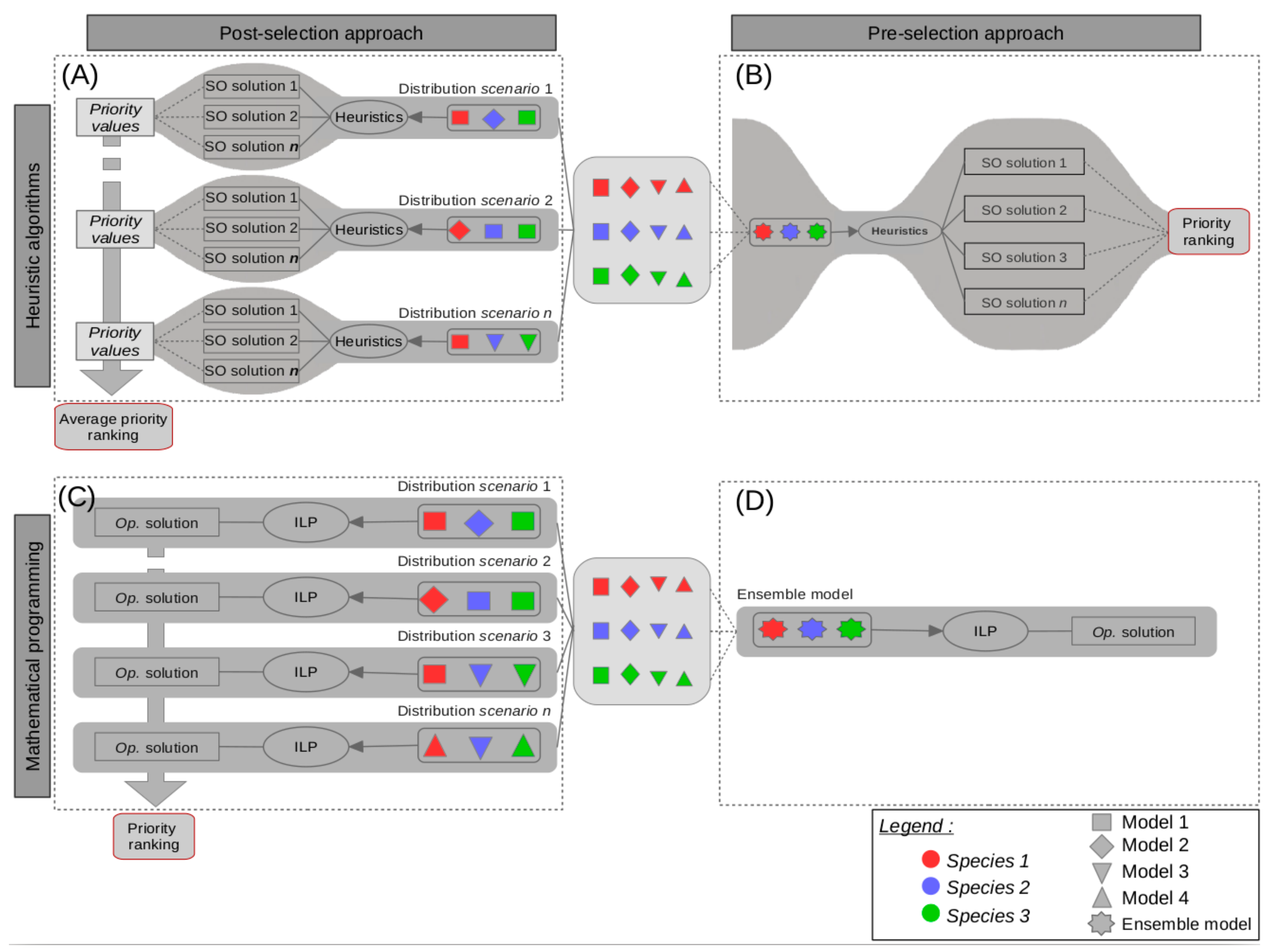
2.3. Conservation Targets, Reserve Selection Algorithms, and Priority Rankings

We defined conservation targets for each data set, as follows: a target of 100% representation was set for species with restricted distribution (range <1000 km²) and a target of 10% was used for extended species (those with a geographic extent exceeding the two-thirds range of the species). For intermediate-sized species, the target was interpolated as a linear function of the log-transformed range area. In addition, we modified area-based targets for critically endangered species, as determined by the IUCN Red List categories, and targeted protecting 100% of their spatial range.

We identified conservation solutions that ensured species representation, while minimizing the total area of selected PUs, following the minimum set problem formulation [49,50]. We used an exact optimization algorithm to solve an integer linear programming problem (ILP; Figure 1C,D; [51]); and the Marxan decision support tool, implementing a random-based heuristic algorithm (Figure 1A,B).

The ILP problem was formulated to minimize an objective function, giving the cost of the solution, while respecting a set of linear constraints:

$$\begin{gathered} \mathrm{Minimize} {\sum }_{i=1}^M{s}_i.x_i \\ \mathrm{subject} \mathrm{to}{\sum }_{i=1}^M{x}_i.a_{ij}\ge t_j\forall j\in E \\ {x}_i\in \left\{0,1\right\} \end{gathered}$$

where M is the number of PUs and E is the set of species. Let a_ij = 1 if species (j ∈ E) is present in PU (i ∈ S) and zero otherwise. The Boolean variable x_i = 1 if the PU (i ∈ S) is selected and zero otherwise. Each PU (i ∈ S) is described by a surface area, s_i and t_j is the minimum amount of each species range to be included in the solution (i.e., the conservation target of species (j ∈ E)). The ILP problems were solved using the GUROBI software, which implements the ‘branch and bound’ exact algorithm [52].

We used Marxan [33], which implements a simulated annealing algorithm (a meta-heuristic algorithm) to identity sub-optimal systems of priority areas. Marxan iteratively minimizes an objective function that sums the total cost of PUs in the solution and penalties for species targets not being met (species’ penalty factor, SPF, species specific weights here set such as to ensure the representation of all species). We set the boundary length modifier to 0 (a parameter that measures the trade-off between cost and compactness of the solution), as our aim was to examine differences in the selection of priority areas among the strategies and not to design an MPA network with a desirable level of compactness. In our study, Marxan was run 100 times and consisted of 1,000,000 iterations per run. In addition, the cost of each site was equal to its area, favoring the selection of sites with high ecological importance.

A priority ranking for planning units was calculated as the selection frequency of each site across a number of conservation solutions, sites selected in more than 90% of the solutions were considered as high-priority conservation areas [53]. For the post-selection approach coupled with heuristic (Figure 1A), the priority rankings obtained for the different distribution scenarios were averaged among the 100 scenarios and 100 Marxan runs. For the pre-selection approach coupled with heuristic optimization (Figure 1B), we calculated the PU selection frequency across the 100 sub-optimal solutions derived from Marxan outputs. For the post-selection approach coupled with exact optimization (Figure 1C), we calculated the selection frequency over the 100 optimal solutions, each based on a different ‘distribution scenario’. For the pre-selection approach coupled with exact optimization (Figure 1D) there is only a single solution.

2.4. Comparative Analysis

First, we compared the distributions of priority rankings (10-bin histograms) derived from the pre-selection approach coupled with a heuristic reserve selection algorithm (the most common strategy, Figure 1B) and the post-selection approach coupled with exact reserve selection algorithm (the unexplored strategy, Figure 1C). To highlight the spatial differences and similarities between priority rankings, we mapped the differences in PUs ranking and measured the overlap in high-priority conservation areas (PUs with irreplaceability >0.9) between the two approaches. We additionally used the Wilcoxon test, known as a t-test for paired samples, to determine statistically significant differences between the rankings obtained. These rankings were compared to the uncertainties associated with the modeling of species distributions using Spearman’s correlation test, to determine whether these uncertainties were better represented by one approach or another.

Additionally, we compared the total protected area for each conservation solution obtained, based on the different approaches, and quantified the efficiency of heuristics outcomes for each ‘distribution scenario’ as the difference in total area with respect to the optimal solution.

3. Results

Overall, the SDMs showed variable performances in predicting observed species distributions, with TSS values ranging from 0 to 0.98 (0.73 ± 0.1; mean ± standard deviation). To avoid spurious conclusions, based on unfair predictions, only models with TSS greater than 0.6 were used for the remaining analyses. For all 438 species considered, several statistical methods reached the performance threshold for predicting observed distributions, which prevented a single ‘better’ model from being distinguished.

In addition, significant variability was observed in the modeled distribution ranges of species (Figure A2). The inferences about species distributions and, consequently, conservation targets are decisively dependent on the SDM modeling approach, with substantial uncertainties associated with the choice of a single best statistical modeling technique. This species-level variability resulted in spatially-structured uncertainties at the assemblage level (Equation (1)), with congruence areas mainly located in pelagic environments; and areas of disagreement at the edge of the species distribution areas, along the margins of the continental shelf, notably along the shores of the Aegean and Ionian seas (Figure 2).

The uncertainties of the SDMs have most often been taken into account in the literature by opting for the pre-selection approach, based on a consensual overall model as input data for SCP (Appendix A). The conservation results based on the pre-selection approach, with the ensemble model as input data for Marxan, revealed that the sub-optimal solutions contained 2.85 to 3.34% more PUs than the optimal solution obtained with ILP. We identified the 32.6% of PUs that were consistently selected across the 100 sub-optimal solutions (Figure A3), while the minimum proportion of PUs required to achieve species targets (i.e., full optimal solution) was 36.7% (Figure A3). Indeed, the distribution of PU selection frequency was strongly bimodal using both exact and heuristics algorithms, with most of the PUs belonging to the first and last 20% quantiles (0–20 and 80–100; Figure 3), reflecting the similarity of the sub-optimal solutions identified using Marxan’s heuristic algorithm.

Following the post-selection approach, 100 ‘distribution scenarios’ were generated by randomly sampling one model for each species among the SDMs selected as having a good predictive performance, thus considering the full range of good predictions (Figure 1A–C). Then, we identified conservation solutions and investigated the variability in their size and in the spatial distribution of the selected PUs. The optimal solutions, each based on a different distribution scenario, varied in size, ranging from c. 27% to c. 43% of the Mediterranean Sea (Figure A3 and Figure A4). Among these optimal solutions, 85% of PUs were selected at least once, with 17% of PUs redundant in 20% to 80% of the solutions. Irreplaceability values derived from the post-selection approach revealed more flexibility than with the pre-selection approach, allocating moderate values (20 to 80) to a greater number of PUs than the pre-selection approach (Figure 3). In this respect, the number of high priority PUs (selected more than 90 times out of the 100 solutions) were about 7% lower than for the pre-selection approach (Figure 3). Moreover, the Wilcoxon tests, used to compare the priority rankings derived from the two pre-selection and post-selection approaches, were significant (p-value < 0.05), revealing that the selection frequency of the PUs depends on the approach followed for considering species distribution uncertainties.

Furthermore, we examined the spatial mismatch of selection frequencies between the two approaches (Figure 4). Only 14% of areas were identified as totally irreplaceable by both approaches (i.e., a selection frequency of 100%; Figure 4). In contrast, the frequency selection of 9.83% of planning units showed differences of 20% and more between the two approaches. Areas with higher priority following the post-selection approach, are mainly located along the Aegean Sea and Ionian Sea coasts; while areas presenting higher priority following the pre-selection approach are spread in small and isolated areas along all Mediterranean coasts (Figure 4). The correlation between SDM uncertainties and the selection frequencies from the post-selection approach was greater than that of the pre-selection approach (Spearman rs 0.77 and 0.57 respectively). Hence, the conservation solutions identified with the post-selection approach were more representative of the uncertainty map of predictions than the pre-selection approach.

The post-selection approach can also be based on sub-optimal solutions, derived from heuristics reserve selection algorithms (Figure 1A). In this study, the statistics on the optimality gaps, calculated between the optimal and sub-optimal solutions for each ‘distribution scenario’, reveal that half of the solutions identified using heuristics are c. 3 to 8% more costly than those found by the exact optimization (Figure 5).

4. Discussion

Systematic conservation planning is a data-intensive process, requiring species occurrence data that fully cover the region of interest [54]. Such knowledge about species distributions is usually so scarce and geographically variable that conservation applications rely increasingly on modeling techniques to predict the distribution of species (Appendix A). The literature review revealed that the choice of the statistical method used to model distributions is likely to be opportunistic in conservation applications, as the great majority of studies identified conservation solutions on the basis of species distributions modeled with only one statistical method. Using a single and a priori chosen model (opportunistically), particularly for rare species, may yield spurious predictions, affecting the selection of MPAs and jeopardizing the adequacy of conservation targets and the representativeness of conservation solutions [55,56]. Before any conservation exercise, it is a good practice to evaluate the predictive performance of SDMs using an evaluation metric (e.g., TSS, AUC). However, while this criterion provides guidance on the relative performance of SDMs, it does not identify the ‘best’ statistical method for distribution modeling. Indeed, the TSS or equivalent measures evaluate the performance of the internal model and, therefore, do not allow deciding on the ecological validity of the predictions [57]. In this study, various models yielded equivalent predictive performances, which prevented distinguishing a single ‘best’ model. It is, thus, good practice for any conservation exercise to start by using different statistical methods for species distribution modeling, and to evaluate the predictive performance of the models obtained [58].

Modeling uncertainties predominate in the literature, and most studies opt for the pre-selection approach, in order to address them (Appendix A; e.g., [41]). Several studies used, to complement SDM ensembles as inputs for SCP, a measure of the variability in species predictions in each cell as a cost. Including uncertainties in SDMs as a constraint for the SCP algorithm implies that sites for which there is low concordance among model predictions are not prioritized [59]. This approach limits the risk of misallocating scarce conservation resources where the uncertainty about the occurrence of species is high. However, as SDMs tend to disagree, particularly for rare species [55,56], it could be that, without further constraints on the representation of rare species (e.g., by adding a strong penalty for the under-representation of rare species in the objective function), places exhibiting a low SDM congruence are the places where most of rare species do occur, potentially decreasing the effective representativeness of conservation solutions for rare species.

The use of an exact reserve selection algorithm to solve an ILP problem based on predictions from the ensemble models (Figure 1D), provided a unique, optimal, and efficient conservation solution covering 36.7% of the Mediterranean Sea and most of the continental shelf (Figure A2). Marxan’s heuristic algorithm produced a set of sub-optimal solutions, making it possible to estimate the priority ranking of PUs (Figure 1B and Figure A3). However, the ranking obtained was strongly bimodal (Figure 3) and geographically structured (Figure A3), with 32.6% of the PUs located over the continental shelf being completely irreplaceable to achieve the conservation objectives. This limits the flexibility offered by heuristics for the implementation of conservation solutions. With this limited flexibility being obtained at the ‘cost’ of efficiency (here 2.85 to 3.34% more sites than the optimal solution), better strategies could be devised to offer flexibility in the implementation of conservation solutions, while optimizing the allocation of conservation resources.

Flexibility can also be provided by applying algorithms repeatedly, under different initial conditions. Following the post-selection approach, different ‘distributions scenarios’ are considered by randomly sampling model predictions for each species among the full range of relevant predictions (Figure 1A–C). Here, the post-selection approach generated priority ranking values with more replaceable PUs and greater flexibility for decision-makers than the pre-selection approach. Furthermore, these rankings were shown to be more representative of species distribution uncertainties than the ones obtained with the pre-selection approach. As such, the post-selection approach coupled with exact optimization represents an alternative to provide both flexibility and efficiency in the SCP process, while acknowledging our limited knowledge of biodiversity distribution.

In practice, this approach can be based on optimal solutions, but also the best sub-optimal solutions from heuristics. Several studies have commented on the sub-optimality of conservation solutions [34,59,60]. Vanderkam et al. (2007) [35] found that heuristics yielded reserve networks that were 2–70% larger than the network identified by an optimal algorithm (e.g., mathematical programming), depending on the formulation of optimization problem and the heuristic algorithm used. Heuristic algorithms cannot inform the user about the degree of sub-optimality of the solutions. Our results show that in the Mediterranean the sub-optimality of Marxan’s solutions can reach up to 8% of the study area (Figure 5). Moilanen (2008) [34] concluded that a 5–10% efficiency loss out of limited resources can be considered meaningful. Combined with the fact that over the 10% of marine areas targeted for protection by the Convention on Biological Diversity only 7.14% of the Mediterranean sea is under a legal conservation designation [60], these results reinforce the need to opt for an algorithm that saves the scarce resources allocated to conservation in this region.

In conclusion, our study highlighted that the modeling technique choice is an important factor to consider when using SDMs as inputs for SCP. The way modeling uncertainties are handled can lead to distinct perspectives on the prioritization of conservation actions and jeopardize the adequacy and representativeness of conservation outcomes. While the pre-selection approach estimates site priorities by varying solutions efficiency, the post-selection approach (coupled with the exact algorithm) provides decision-makers with the greatest information related to the uncertainties in species distributions across different modeling techniques. This information, communicated as priority values, where the most irreplaceable areas are selected across different potential ‘distribution scenarios’ could help to better implement the fundamental principles of SCP, aiming for adaptive and effective management of resources.

References

1. Cardinale, B.J.; Duffy, J.E.; Gonzalez, A.; Hooper, D.U.; Perrings, C.; Venail, P.; Narwani, A.; Mace, G.M.; Tilman, D.; Wardle, D.A.; et al. Biodiversity loss and its impact on humanity. Nature 2012, 486, 59. [Google Scholar] [CrossRef]
2. Worm, B.; Barbier, E.B.; Beaumont, N.; Duffy, J.E.; Folke, C.; Halpern, B.S.; Jackson, J.B.C.; Lotze, H.K.; Micheli, F.; Palumbi, S.R.; et al. Impacts of Biodiversity Loss on Ocean Ecosystem Services. Science 2006, 314, 787–790. [Google Scholar] [CrossRef] [PubMed] [Green Version]
3. Margules, C.R.; Pressey, R.L. Systematic conservation planning. Nature 2000, 405, 243–253. [Google Scholar] [CrossRef]
4. Possingham, H.; Wilson, K.; Andelman, S.; Vynne, C. Protected areas: Goals, limitations, and design. In Principles of Conservation Biology, 3rd ed; Sinauer Associates: Sunderland, MA, USA, 2006; pp. 507–549. [Google Scholar]
5. Magris, R.A.; Pressey, R.L.; Mills, M.; Vila-Nova, D.A.; Floeter, S. Integrated conservation planning for coral reefs: Designing conservation zones for multiple conservation objectives in spatial prioritisation. Global Ecol. Conserv. 2017, 11, 53–68. [Google Scholar] [CrossRef]
6. Davies, T.E.; Maxwell, S.M.; Kaschner, K.; Garilao, C.; Ban, N.C. Large marine protected areas represent biodiversity now and under climate change. Sci. Rep. 2017, 7, 1–7. [Google Scholar] [CrossRef] [Green Version]
7. Drira, S.; Ben Rais Lasram, F.; Ben Rejeb Jenhani, A.; Shin, Y.J.; Guilhaumon, F. Species-area uncertainties impact the setting of habitat conservation targets and propagate across conservation solutions. Biol. Conserv. 2019, 235, 279–289. [Google Scholar] [CrossRef]
8. Araújo, M.B.; Williams, P.H. Selecting areas for species persistence using occurrence data. Biol. Conserv. 2000, 96, 331–345. [Google Scholar] [CrossRef] [Green Version]
9. Araújo, M.B.; Williams, P.H.; Turner, A. A sequential approach to minimise threats within selected conservation areas. Biodivers. Conserv. 2002, 11, 1011–1024. [Google Scholar] [CrossRef]
10. Harnik, P.G.; Lotze, H.K.; Anderson, S.C.; Finkel, Z.V.; Finnegan, S.; Lindberg, D.R.; Liow, L.H.; Lockwood, R.; McClain, C.R.; McGuire, J.L.; et al. Extinctions in ancient and modern seas. Trends Ecol. Evol. 2012, 27, 608–617. [Google Scholar] [CrossRef]
11. Rodrigues, A.S.L.; Andelman, S.J.; Bakarr, M.I.; Boitani, L.; Brooks, T.M.; Cowling, R.M.; Fishpool, L.D.C.; da Fonseca, G.A.B.; Gaston, K.J.; Hoffmann, M.; et al. Effectiveness of the global protected area network in representing species diversity. Nature 2004, 428, 640–643. [Google Scholar] [CrossRef]
12. Bini, L.M.; Diniz-Filho, J.A.F.; Rangel, T.F.L.V.B.; Bastos, R.P.; Pinto, M.P. Challenging Wallacean and Linnean shortfalls: Knowledge gradients and conservation planning in a biodiversity hotspot. Divers. Distrib. 2006, 12, 475–482. [Google Scholar] [CrossRef]
13. Lomolino, M. Conservation biogeography. In Frontiers of Biogeography: New Directions in the Geography of Nature, 293; Sinauer Associates, Inc.: Sunderland, MA, USA, 2004. [Google Scholar]
14. Terribile, L.C.; Lima-Ribeiro, M.S.; Araujo, M.B.; Bizao, N.; Collevatt, R.G.; Dobrovolski, R.; Diniz Filho, J.A.F. Areas of climate stability of species ranges in the Brazilian Cerrado: Disentangling uncertainties through time. Nat. Conserv. 2012, 10, 152–159. [Google Scholar] [CrossRef]
15. Whittaker, R.J.; Araújo, M.B.; Jepson, P.; Ladle, R.J.; Watson, J.E.; Willis, K.J. Conservation biogeography: Assessment and prospect. Divers. Distrib. 2005, 11, 3–23. [Google Scholar] [CrossRef]
16. Elith, J.; Leathwick, J.R. Species Distribution Models: Ecological Explanation and Prediction Across Space and Time. Annu. Rev. Ecol. Evol. Syst. 2009, 40, 677–697. [Google Scholar] [CrossRef]
17. Marmion, M.; Parviainen, M.; Luoto, M.; Heikkinen, R.K.; Thuiller, W. Evaluation of consensus methods in predictive species distribution modelling. Divers. Distrib. 2009, 15, 59–69. [Google Scholar] [CrossRef]
18. Wisz, M.S.; Hijmans, R.J.; Li, J.; Peterson, A.T.; Graham, C.H.; Guisan, A. NCEAS Predicting Species Distributions Working Group†. Effects of sample size on the performance of species distribution models. Divers. Distrib. 2008, 14, 763–773. [Google Scholar] [CrossRef]
19. Elith, J.H.; Graham, C.P.; Anderson, R.; Dudík, M.; Ferrier, S.; Guisan, A.J.; Hijmans, R.; Huettmann, F.R.; Leathwick, J.; Lehmann, A.; et al. Novel methods improve prediction of species’ distributions from occurrence data. Ecography 2006, 29, 129–151. [Google Scholar] [CrossRef] [Green Version]
20. Guisan, A.; Zimmermann, N.E.; Elith, J.; Graham, C.H.; Phillips, S.; Peterson, A.T. What matters for predicting the occurrences of trees: Techniques, data, or species characteristics? Ecol. Monogr. 2007, 77, 615–630. [Google Scholar] [CrossRef] [Green Version]
21. Roura-Pascual, N.; Brotons, L.; Peterson, A.T.; Thuiller, W. Consensual predictions of potential distributional areas for invasive species: A case study of Argentine ants in the Iberian Peninsula. Biol. Invasions 2009, 11, 1017–1031. [Google Scholar] [CrossRef]
22. Lentini, P.E.; Wintle, B.A. Spatial conservation priorities are highly sensitive to choice of biodiversity surrogates and species distribution model type. Ecography 2015, 38, 1101–1111. [Google Scholar] [CrossRef]
23. Loiselle, B.A.; Howell, C.A.; Graham, C.H.; Goerck, J.M.; Brooks, T.; Smith, K.G.; Williams, P.H. Avoiding Pitfalls of Using Species Distribution Models in Conservation Planning. Conserv. Biol. 2003, 17, 1591–1600. [Google Scholar] [CrossRef]
24. Haight, R.G.; Revelle, C.S.; Snyder, S.A. An Integer Optimization Approach to a Probabilistic Reserve Site Selection Problem. Oper. Res. 2000, 48, 697–708. [Google Scholar] [CrossRef] [Green Version]
25. Wilson, K.A.; Cabeza, M.; Klein, C.J. Fundamental concepts of spatial conservation prioritization. In Spatial Conservation Prioritization: Quantitative Methods and Computational Tools; Oxford University Press: New York, NY, USA, 2009; pp. 16–27. [Google Scholar]
26. Sarkar, S. Ecological Diversity and Biodiversity as Concepts for Conservation Planning: Comments on Ricotta. Acta Biotheor. 2006, 54, 133–140. [Google Scholar] [CrossRef] [PubMed]
27. Camm, J.D.; Polasky, S.; Solow, A.; Csuti, B. A note on optimal algorithms for reserve site selection. Biol. Conserv. 1996, 78, 353–355. [Google Scholar] [CrossRef]
28. Önal, H. First-best, second-best, and heuristic solutions in conservation reserve site selection. Biol. Conserv. 2004, 115, 55–62. [Google Scholar] [CrossRef]
29. Underhill, L.G. Optimal and suboptimal reserve selection algorithms. Biol. Conserv. 1994, 70, 85–87. [Google Scholar] [CrossRef]
30. Jantke, K.; Jones, K.R.; Allan, J.R.; Chauvenet, A.L.; Watson, J.E.; Possingham, H.P. Poor ecological representation by an expensive reserve system: Evaluating 35 years of marine protected area expansion. Conserv. Lett. 2018, 11, e12584. [Google Scholar] [CrossRef] [Green Version]
31. Hanson, J.O.; Rhodes, J.R.; Butchart, S.H.; Buchanan, G.M.; Rondinini, C.; Ficetola, G.F.; Fuller, R.A. Global conservation of species’ niches. Nature 2020, 580, 232–234. [Google Scholar] [CrossRef] [PubMed]
32. Wilhere, G.F.; Goering, M.; Wang, H. Average optimacity: An index to guide site prioritization for biodiversity conservation. Biol. Conserv. 2008, 141, 770–781. [Google Scholar] [CrossRef]
33. Ball, I.R.; Possingham, H.P.; Watts, M. Marxan and relatives: Software for spatial conservation prioritisation. In Spatial Conservation Prioritisation: Quantitative Methods and Computational Tools; Oxford University Press: Oxford, UK, 2009; pp. 185–195. [Google Scholar]
34. Moilanen, A. Two paths to a suboptimal solution—once more about optimality in reserve selection. Biol. Conserv. 2008, 141, 1919–1923. [Google Scholar] [CrossRef]
35. Vanderkam, R.P.D.; Wiersma, Y.F.; King, D.J. Heuristic algorithms vs. linear programs for designing efficient conservation reserve networks: Evaluation of solution optimality and processing time. Biol. Conserv. 2007, 137, 349–358. [Google Scholar] [CrossRef]
36. Bailey, H.; Thompson, P. Using marine mammal habitat modelling to identify priority conservation zones within a marine protected area. Mar. Ecol. Prog. Ser. 2009, 378, 279–287. [Google Scholar] [CrossRef] [Green Version]
37. Leach, K.; Zalat, S.; Gilbert, F. Egypt’s Protected Area network under future climate change. Biol. Conserv. 2013, 159, 490–500. [Google Scholar] [CrossRef]
38. Passoni, G.; Rowcliffe, J.M.; Whiteman, A.; Huber, D.; Kusak, J. Framework for strategic wind farm site prioritisation based on modelled wolf reproduction habitat in Croatia. Eur. J. Wildl. Res. 2017, 63, 38. [Google Scholar] [CrossRef]
39. Walther, B.A.; Pirsig, L.H. Determining conservation priority areas for Palearctic passerine migrant birds in sub-Saharan Africa. Avian Conserv. Ecol. 2017, 12, 2. [Google Scholar] [CrossRef] [Green Version]
40. Zhang, L.; Liu, S.; Sun, P.; Wang, T.; Wang, G.; Zhang, X.; Wang, L. Consensus Forecasting of Species Distributions: The Effects of Niche Model Performance and Niche Properties. PLoS ONE 2015, 10, e0120056. [Google Scholar] [CrossRef] [PubMed] [Green Version]
41. Bush, A.; Hermoso, V.; Linke, S.; Nipperess, D.; Turak, E.; Hughes, L. Freshwater conservation planning under climate change: Demonstrating proactive approaches for Australian Odonata. J. Appl. Ecol. 2014, 51, 1273–1281. [Google Scholar] [CrossRef]
42. Meller, L.; Cabeza, M.; Pironon, S.; Barbet-Massin, M.; Maiorano, L.; Georges, D.; Thuiller, W. Ensemble distribution models in conservation prioritization: From consensus predictions to consensus reserve networks. Divers. Distrib. 2014, 20, 309–321. [Google Scholar] [CrossRef] [PubMed]
43. Ben Rais Lasram, F.; Guilhaumon, F.; Mouillot, D. Fish diversity patterns in the Mediterranean Sea: Deviations from a mid-domain model. Mar. Ecol. Prog. Ser. 2009, 376, 253–267. [Google Scholar] [CrossRef] [Green Version]
44. Ben Rais Lasram, F.; Guilhaumon, F.; Albouy, C.; Somot, S.; Thuiller, W.; Mouillot, D. The Mediterranean Sea as a ‘cul-de-sac’ for endemic fishes facing climate change. Glob. Change Biol. 2010, 16, 3233–3245. [Google Scholar] [CrossRef]
45. Albouy, C.; Guilhaumon, F.; Leprieur, F.; Ben Rais Lasram, F.; Somot, S.; Aznar, R.; Velez, L.; Le Loc’h, F.; Mouillot, D. Projected climate change and the changing biogeography of coastal Mediterranean fishes. J. Biogeogr. 2013, 40, 534–547. [Google Scholar] [CrossRef]
46. Albouy, C.; Ben Rais Lasram, F.; Velez, L.; Guilhaumon, F.; Meynard, C.N.; Boyer, S.; Mouillot, D. FishMed: Traits, phylogeny, current and projected species distribution of Mediterranean fishes, and environmental data: Ecological Archives E096-203. Ecology 2015, 96, 2312–2313. [Google Scholar] [CrossRef] [Green Version]
47. Thuiller, W.; Georges, D.; Engler, R.; Breiner, F.; Georges, M.D.; Thuiller, C.W. Package ‘biomod2′. Species distribution modeling within an ensemble forecasting framework. Ecography 2016, 32, 369–373. [Google Scholar] [CrossRef]
48. Allouche, O.; Tsoar, A.; Kadmon, R. Assessing the accuracy of species distribution models: Prevalence, kappa and the true skill statistic (TSS): Assessing the accuracy of distribution models. J. Appl. Ecol. 2006, 43, 1223–1232. [Google Scholar] [CrossRef]
49. Guilhaumon, F.; Albouy, C.; Claudet, J.; Velez, L.; Ben Rais Lasram, F.; Tomasini, J.-A.; Douzery, E.J.; Meynard, C.N.; Mouquet, N.; Troussellier, M.; et al. Representing taxonomic, phylogenetic and functional diversity: New challenges for Mediterranean marine-protected areas. Divers. Distrib. 2015, 21, 175–187. [Google Scholar] [CrossRef]
50. Moilanen, A.; Ball, I. Heuristic and approximate optimization methods for spatial conservation prioritization. In Spatial Conservation Prioritization: Quantitative Methods and Computational Tools; Moilanen, A., Wilson, K.A., Possingham, H.P., Eds.; Oxford University Press: New York, NY, USA, 2009; pp. 58–69. [Google Scholar]
51. Possingham, H.; Ball, I.; Andelman, S. Mathematical methods for identifying representative reserve networks. In Quantitative Methods for Conservation Biology; Springer: New York, NY, USA, 2000; pp. 291–306. Available online: https://link.springer.com/book/10.1007/b97704 (accessed on 24 December 2021).
52. Gurobi Optimization; Gurobi Optimization. Inc.: Houston, TX, USA, 2012.
53. Andelman, S.J.; Willig, M.R. Alternative configurations of conservation reserves for Paraguayan bats: Considerations of spatial scale. Conserv. Biol. 2002, 16, 1352–1363. [Google Scholar] [CrossRef] [Green Version]
54. Tulloch, A.I.T.; Sutcliffe, P.; Naujokaitis-Lewis, I.; Tingley, R.; Brotons, L.; Ferraz, K.M.; Possingham, H.; Guisan, A.; Rhodes, J.R. Conservation planners tend to ignore improved accuracy of modelled species distributions to focus on multiple threats and ecological processes. Biol. Conserv. 2016, 199, 157–171. [Google Scholar] [CrossRef] [Green Version]
55. Guillera-Arroita, G.; Lahoz-Monfort, J.J.; Elith, J.; Gordon, A.; Kujala, H.; Lentini, P.E.; McCarthy, M.A.; Tingley, R.; Wintle, B.A. Is my species distribution model fit for purpose? Matching data and models to applications. Glob. Ecol. Biogeogr. 2015, 24, 276–292. [Google Scholar] [CrossRef]
56. Pearson, R.G.; Thuiller, W.; Araújo, M.B.; Martinez-Meyer, E.; Brotons, L.; McClean, C.; Miles, L.; Segurado, P.; Dawson, T.P.; Lees, D.C. Model-based uncertainty in species range prediction. J. Biogeogr. 2006, 33, 1704–1711. [Google Scholar] [CrossRef]
57. Porfirio, L.L.; Harris, R.M.B.; Lefroy, E.C.; Hugh, S.; Gould, S.F.; Lee, G.; Bindoff, N.L.; Mackey, B. Improving the Use of Species Distribution Models in Conservation Planning and Management under Climate Change. PLoS ONE 2014, 9, e113749. [Google Scholar] [CrossRef] [Green Version]
58. Molloy, S.; Davis, R.; Van Etten, E. An evaluation and comparison of spatial modelling applications for the management of biodiversity: A case study on the fragmented landscapes of south-Western Australia. Pac. Conserv. Biol. 2016, 22, 338–349. [Google Scholar] [CrossRef]
59. Pressey, R.L.; Possingham, H.P.; Margules, C.R. Optimality in reserve selection algorithms: When does it matter and how much? Biol. Conserv. 1996, 76, 259–267. [Google Scholar] [CrossRef] [Green Version]
60. MAPAMED, the database of MArine Protected Areas in the MEDiterranean. 2019 edition. © 2020 by SPA/RAC and MedPAN, Licensed under CC BY-NC-SA 4.0. Available online: https://www.mapamed.org/ (accessed on 18 June 2019).
Figure 1. Schematic representation of the different approaches for the definition of spatial priorities when accounting for species distribution model uncertainties. For each species (represented by different colors), the spatial distribution is modeled using various statistical methods (each represented by a different shape), from this pool of species/method predictions (central gray squares), four approaches are possible. The first two approaches use random-based heuristics, to identify conservation solutions. (A) A post-selection approach, where a set of sub-optimal solutions are generated for different distribution scenarios, each constructed by selecting randomly a model among all SDMs for each species. Priority rankings corresponding to different distribution scenarios are then summarized by averaging. (B) A pre-selection approach, where species distribution models are summarized into a unique ensemble model before reserve selection. The priority ranking is estimated from several sub-optimal solutions. The two latter approaches use exact optimization. (C) A post-selection approach, where priority ranking values are estimated for a set of optimal solutions, each corresponding to a different distribution scenario. (D) A pre-selection approach of SDM outputs (ensembling), leading to a unique optimal solution. The way uncertainties related to both model accuracy and solution efficiency spread across the SCP process is illustrated by gray shades of different heights in each panel.
Diversity 14 00009 g001
Figure 2. Map of assemblage-level uncertainties in SDM predictions. Uncertainty is calculated at the species level (Equation (1)) and averaged across species present in each planning unit. Green areas indicate cells for which model prediction uncertainties are the highest.
Diversity 14 00009 g002
Figure 3. Frequency distributions of priority ranking values derived from the two approaches used for integrating species distribution uncertainties. Bars of full color represent the result of the post-selection approach coupled with exact optimization, hatched bars represent the result from the pre-selection approach coupled with heuristics. The curve represents the frequency differences across different levels of priority between the two approaches.
Diversity 14 00009 g003
Figure 4. Comparison of priority ranking values based on the two approaches, including uncertainty associated with distribution modeling. Map of difference in planning unit (PU) selection frequency. Scatter plot showing the PU selection frequency under the different approaches. Histogram of selection frequency differences.
Diversity 14 00009 g004
Figure 5. Left: scatter plot showing the area of conservation solutions (expressed as percentage of the sea) for random-based heuristics and optimal conservation outcomes for both the pre-selection and post-selection approaches; each point represents the percentage of protected areas necessary to achieve species target. Right: boxplot of optimality gap between sub-optimal and optimal conservation outcomes for each ‘distribution scenario’. The gap between the best Marxan solution and the optimal solution based on the pre-selection approach is shown by a red point.
Diversity 14 00009 g005
Publisher’s Note: MDPI stays neutral with regard to jurisdictional claims in published maps and institutional affiliations.