Article

Estimated Density, Population Size and Distribution of the Endangered Western Hoolock Gibbon (Hoolock hoolock) in Forest Remnants in Bangladesh

1
Department of Zoology, Jagannath University, Dhaka 1100, Bangladesh
2
Department of Biology, United Arab Emirates University, Al Ain P.O. Box 15551, United Arab Emirates
*
Author to whom correspondence should be addressed.
Diversity 2021, 13(10), 490; https://doi.org/10.3390/d13100490
Submission received: 9 September 2021 / Revised: 2 October 2021 / Accepted: 4 October 2021 / Published: 6 October 2021
(This article belongs to the Section Biodiversity Conservation)

Abstract

:
Tropical forests are threatened worldwide due to deforestation. In South and Southeast Asia, gibbons (Hylobatidae) are important to seed dispersal and forest regeneration. Most gibbons are threatened due to deforestation. We studied the western hoolock gibbon (Hoolock hoolock) in Bangladesh to determine population size and extent of suitable habitat. We used distance sampling to estimate density across 22 sites in northeastern and southeastern Bangladesh. We used Maxent modeling to determine areas of highly suitable habitat throughout Bangladesh. Density was estimated to be 0.39 ± 0.09groups/km2, and the total estimated population was 468.96 ± 45.56 individuals in 135.31 ± 2.23 groups. The Maxent model accurately predicted gibbon distribution. Vegetation cover, isothermality, annual precipitation, elevation and mean temperature of the warmest quarter influenced distribution. Two areas in the northeast and two areas in the southeast have high potential for gibbon conservation in Bangladesh. We also found significantly more gibbons in areas that had some level of official protection. Thus, we suggest careful evaluation, comprehensive surveys and restoration of habitats identified as suitable for gibbons. We recommend bringing specific sites in the northeastern and southeastern regions under protection to secure habitat for remaining gibbon populations.

1. Introduction

Global forest cover has declined over the period of 1900–2000 at a rate of about 3.1% per year, with forests currently occupying less than 4 million km2 of Earth [1,2]. Dense human populations continue to exert immense pressures on forests in the tropics [1,3,4]. As a result, deforestation rates have remained high in the tropics [1]. Tropical forests in South Asia have been classified variously into a range of tropical moist, tropical evergreen and several other forest types based on vegetational composition [2,5]. Forestry practices in the Indian Subcontinent and the Southeast Asian regions initiated in the colonial era (prior to World War II) have been responsible for alteration of tree species composition. Replacement of diverse tree species assemblages with selected tree species (such as teak, Tectonia grandis, and sal, Shorearobusta) for plantations has been causing slow and systematic decline in forest species diversity in South Asia. In comparison, palm oil plantations have become a dominating force in the decline of forest diversity in Southeast Asia [1]. Currently, about 79 million hectares of forests remain in South Asia [1], where about 23% of the world’s population also resides. Thus, most of the emphasis on forest conservation goes towards treating forests as a resource rather than understanding its overall biodiversity value. Currently, most of the South Asian forests (especially in India and Bangladesh) have become converted for agriculture or development, retaining relatively small pockets of forest surrounded by a mosaic of agroforestry or agricultural landscapes [1,6,7,8].
Primates form a major component of many tropical forests. Among the primates, gibbons (Hylobatidae) are a particularly threatened family, with 14 of the 19 species being either endangered or critically endangered as listed in the International Union for the Conservation of Nature (IUCN) [9,10,11,12]. Most gibbon species occur in Southeast Asia, with only two species occurring in South Asia (in India and Bangladesh). Gibbons play central roles in seed dispersal and forest regeneration due to their frugivorous diets [13,14]. They generally avoid descending to the forest floor, and their brachiating movement requires contiguous forest with closed canopy tree structure [6,9]. Forest degradation, compositional change, fragmentation, isolation and loss represent major threats to all gibbon species [9,10,11,12,13,14].
Hoolock is the only gibbon genus that occurs in the Indian subcontinent with three recognized species [7,15,16,17]. The western hoolock gibbon (Hoolock hoolock) occurs west of Chindwin River in India, eastern Bangladesh and northwestern Myanmar. There are less than 2600 individuals of H. hoolock in India, mostly in Assam [18] and 200–300 in Bangladesh [7], making the species globally endangered [10]. At the western edge of their distributional range in Bangladesh, they are nationally listed as critically endangered, with generally declining population trends [19,20]. Western hoolock gibbons are threatened throughout their distribution by habitat destruction and degradation, poaching for food or medicinal products, capture of individuals for the illegal wildlife trade (pets), mining activities in forests and urban development [21,22].
The first population estimate from the 1980s suggested a population of 3000 individuals in roughly 900 groups [22], although the authors did not mention estimation methods. There was substantially more forest cover in the 1980s compared to the 1990s, suggesting that the estimate by Gittins and Akonda [22] was realistic. Subsequent population estimates suggested around 200 individuals in about 55 groups in the early 1990s [23] and 282 individuals in 96 groups in the early 2000s [7]. This is consistent with rapid forest declines during the 1980s [4,8]. The latter estimates [7,23] were possibly underestimates since many areas were not surveyed. Das et al. [24] summarized the distribution of western hoolock gibbons in Bangladesh, identifying 14 sites that still retained western hoolock gibbons. The survey by Islam et al. [7] was the most comprehensive in terms of sites visited (35 sites of which 25 had western hoolock gibbon populations). However, minimum population size was estimated (i.e., only individuals in groups that were seen or heard calling were included in the estimate) making the estimate low.
Forest cover and connectivity has changed since the last assessment. The total national forest cover is over 15,000 km2 (roughly 10.3% of the total area of Bangladesh) [3,4]. The northeastern and southeastern regions of Bangladesh consist of about 4870 km2 of mixed evergreen and hill forests [3,4]. Although tree cover has generally increased in Bangladesh due to village forest plantations (composed of primarily exotic tree species), forest cover has continued to decrease, resulting in a net loss of biodiversity [4]. All forests in Bangladeshi sites are severely degraded with comparable levels of disturbance [3,6]. Gibbon habitats consisting of dense, closed canopy forests are found mostly in southeastern Asia [25,26]. In Bangladesh, areas with gibbon populations are far poorer in quality and extent of occurrence compared to the Southeast Asian forests [1,6,8]. Thus, we anticipate a decrease in western hoolock gibbon populations in Bangladesh consistent with a decline in overall forest cover between 2006 and 2020.
Presence/absence data has been widely used in recent years to determine potential distribution and ecology of a variety of species including primates [27,28,29,30]. Maximum Entropy Modeling (Maxent) has become popular because it uses presence only data integrated with environmental variables to generate potential species distributional ranges [27,28]. Maxent models accurately predict distributions as well as highlight areas with similar characteristics where a primate species could occur. This has included endangered or critically endangered species on which high quality abundance data is lacking [31,32]. Furthermore, Maxent models can also test important ecological questions related to landscape characteristics, seed dispersal or movement ecology to predict threats on primates and help propose conservation action [30,33]. Sarma et al. [34] modelled the distribution of Hoolock leuconedys in northeastern India using Maxent as well as other vegetation indices. Similarly, Alamgir et al. [35] and Sarma et al. [36] modelled the distribution of H. hoolock in Bangladesh and northeastern India, respectively, in Maxent along with land use-land cover (LULC) and other indices demonstrating the predictive power of Maxent for Hoolock gibbons. Thus, Maxent modeling of hoolock gibbon distribution in Bangladesh could identify areas of high value suitable for conservation of the species. This is particularly important since habitat suitable for gibbons has been lost since the early 2000s [4,8], suggesting that the overall area of occupancy of the species has declined.
We conducted population surveys across known western hoolock gibbon habitats in Bangladesh. The objectives of this study were to (i) estimate the total population of western hoolock gibbons in 22 sites in Bangladesh; and (ii) determine the current distribution of western hoolock gibbons in Bangladesh using species distribution modeling.

2. Materials and Methods
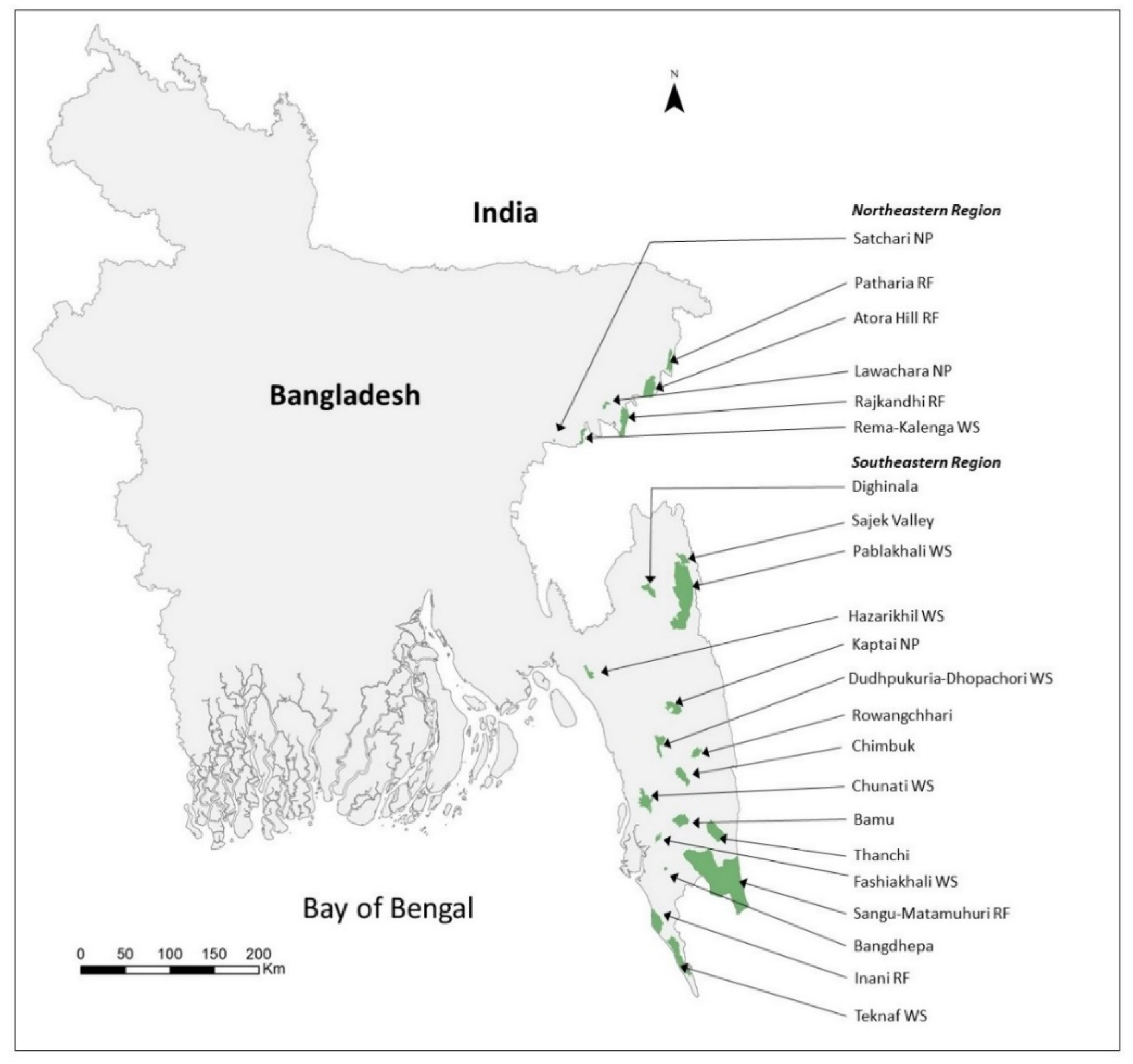
2.1. Study Sites

Western hoolock gibbon populations were surveyed in northeastern and southeastern Bangladesh (Figure 1). Western hoolock gibbons select closed canopy forests composed of a variety of tree species and forests in the northeastern and southeastern regions that are characterized by a hilly topography with species of Quercus, Syzygium, Gmelina, Ficus, Artocarpus and Dipterocarpus forming diverse tree communities [6,7]. Islam et al. [7] chose 35 sites based on historical presence of western hoolock gibbons and presence of closed-canopy forest cover [6,7]. Twenty two sites from these 35 were chosen for our study, since the remaining sites did not have gibbon populations [7,18,19,24].

2.2. Population Surveys

We used distance sampling to estimate western hoolock gibbon populations. Attempts were made to visit each site for at least 3 days, although this was not always possible or needed. For example, some sites were small (<5 km2) making it easy to confirm the presence or absence of western hoolock gibbons and conduct transect counts. Larger sites were visited for longer periods and one site could not be visited for more than one day due to logistical and security issues. At each site, transects were walked at a speed of approximately 1.5 km/h by 2–3 people (including at least one of the authors), trained and experienced in detecting western hoolock gibbons from 0500h to 1500h based on activity patterns of the species [23]. Once an individual was detected, its location in relation to the transect was determined using a rangefinder (SUAOKI Digital Laser Rangefinder Scope 5-600P, China) that provided distance from the observer and the angle modified from Muzaffar et al. [6]. The perpendicular distance between the western hoolock gibbon and the observer on the transect was determined following standard trigonomeric methods consistent with standard distance sampling theory [6]. All the authors involved in fieldwork had prior experience detecting western hoolock gibbons and evaluating group size, composition and using distance sampling protocols. All authors and additional field assistants were further trained by the senior authors at Lawachara National Park (henceforth referred to as NP) in March 2019.
Lawachara NP was visited for 17 days, as it is much easier to access and a total population count of the site was possible. This was used to help validate our estimate of density from the distance sampling method (see below). About seven forest areas (with areas of suitable habitat <5km2) were far more degraded and we determined total number of groups of western hoolock gibbons were either counted or obtained from forest officials. Although we did walk transects for these sites, we used the actual known counts for density estimates. A total of 1–7 transects were selected at each site. Each transect was either an existing forest trail or a dry stream bed (common in many of the stream-fed forests). Transects were chosen haphazardly with an effort to spread them as far apart as possible to attain as representative coverage of the forest patch as possible. A total of 204.65 km of transects were walked to conduct the surveys. Most forest patches were small in size with patch size ranging from 2.35–69.03 km2.

2.3. Modelling Group Density

We built a Bayesian probability model for the number of groups observed at each transect and their perpendicular distance from the transect in RStan [37]. We modelled the probability distribution of the distance with a half-normal distribution in order to estimate the effective distance w. Effective area of observation, E, was estimated as follows from integrating the half normal:
E = w 2 π
We then modelled the probability distribution of groups with a Poisson distribution [38] with a scale parameter that resulted from multiplying the effective area of observation by the group density. Therefore, each detected group contributed to the global probability with a value coming from the distance and a value from its detection. This procedure extracts the same information as using distance categories [39], without the hassle of having to decide which distance categories to use.
We considered a single value of effective area of observation for all the sites, and we allowed the densities to vary from site to site. We modelled the distribution of the logarithm of the site densities with a normal distribution. We used normal distributions for all prior probability distributions (henceforth referred to as priors), using a logarithm transformation for all the mandatory positive parameters (like densities and all the variances). Thus, the mean and standard deviation of the logarithm of the group densities was log m and log f, respectively. This meant that the 68% of the sites would have a density between m/f and mf. However, we were uncertain on the values of m and f, so we modelled this uncertainty again with a normal distribution of m and of log f. This hyper-parameter models our knowledge (i.e., a mean and a standard deviation) in the variability in the density among sites. Therefore, a value of log (log a) in the mean and a value of log r in the standard deviation would indicate that the variability on the densities of sites would have values of ma-r and mar.

2.4. Habitat Suitability and Population Size

We downloaded land-use/land-cover (LULC) from the European Space Agency-climate change initiative-Land Cover (version 2.1.1) [40] for the year 2019 at 300m resolution. Land-use/land-cover data from Bangladesh identifies four categories of tree cover that we consider to be suitable forest cover, namely: (i) tree cover, broad leaved, evergreen, (ii) tree cover, broadleaved, deciduous, (iii) tree cover, needle leaved, evergreen, and (iv) tree cover, needle-leaved, deciduous. These were collectively pooled as ‘forest cover’ and are consistent with scattered forest patches in the central and northern parts (consistent with Shorearobusta or sal forests), mangrove forests located in the southwest, and mixed evergreen/deciduous forests (known as hill forests) in the northeastern and southeastern regions [4]. We obtained the areas classified as forest cover in the northeastern and southeastern regions to determine the extent of coverage of forests in our 22 study sites. We calculated the area of forest cover within each of the 22 study sites using the spatial analyst tool in ArcGIS (Desktop 10.8.1) [41]. We used the LULC variables for Maxent modeling (see below). We also plotted the shape files for each of the 22 sites on Google Earth Pro to individually classify and plot forest cover using drawing tools in Google Earth Pro [42]. We verified the occurrence of forests while we surveyed in those areas to make sure that the Google Earth images were in fact ‘forests’ and not an artefact of poor image quality. A detailed assessment of habitat was not possible. We ground truthed 20 of the 22 sites. Ground truthing was carried out for about 10–30% of the total area of the forest. Classification error rate based on ground truthing varied between sites and ranged from 5–20%. Areas that appeared to have closed canopy and mixed tree species on Google Earth but were in reality composed of teak or other monoculture plantations were excluded from the maps after ground truthing, where possible. The resulting shape files of forest cover within each study site were then used to estimate the area of forest cover using Earth Point [43].
The final total area of forest cover obtained from this method was typically less than the area defined by LULC methods, although there were a few exceptions. We defined ‘suitable’ habitat as those having mixed fruiting trees and connectivity between tree crowns [6] and were classified as forest cover as estimated in our method using Google Earth. The group density estimates for each site were then multiplied by the available suitable habitat at each site to derive number of groups. Population size was derived from individual group densities to the mean number of individuals per group recorded in our study. We used group density of individual sites as a response variable and protected status (national park, wildlife sanctuary, reserved forest or not protected) as an explanatory variable to run a one-way ANOVA to assess if protection had an effect on population density.

2.5. Preprocessing of Variables for Habitat Assessment

We further assessed habitat using an ecological niche modelling approach. We selected 19 bioclimatic, elevation and land-use/land cover (LULC) variables initially. The bioclimatic variables were downloaded from WorldClim database (version 1.4) at 30-arc-second (~ 1 km) resolution [44]. Elevation data was obtained from NOAA Digital Elevation Map (DEM) [45] with the same spatial resolution as the bioclimatic variables. We clipped all selected factors (Table 1) to the Bangladesh area and processed it to have the same cell size and spatial extent (nearest neighbor resampling method) using ArcGIS. We assessed multicollinearity between the 19 bioclimatic variables using Variance Inflation Factor analyses (VIF) in R (version 4.0.2). We eliminated highly correlated variables considering a VIF >10 as a critical threshold [46].

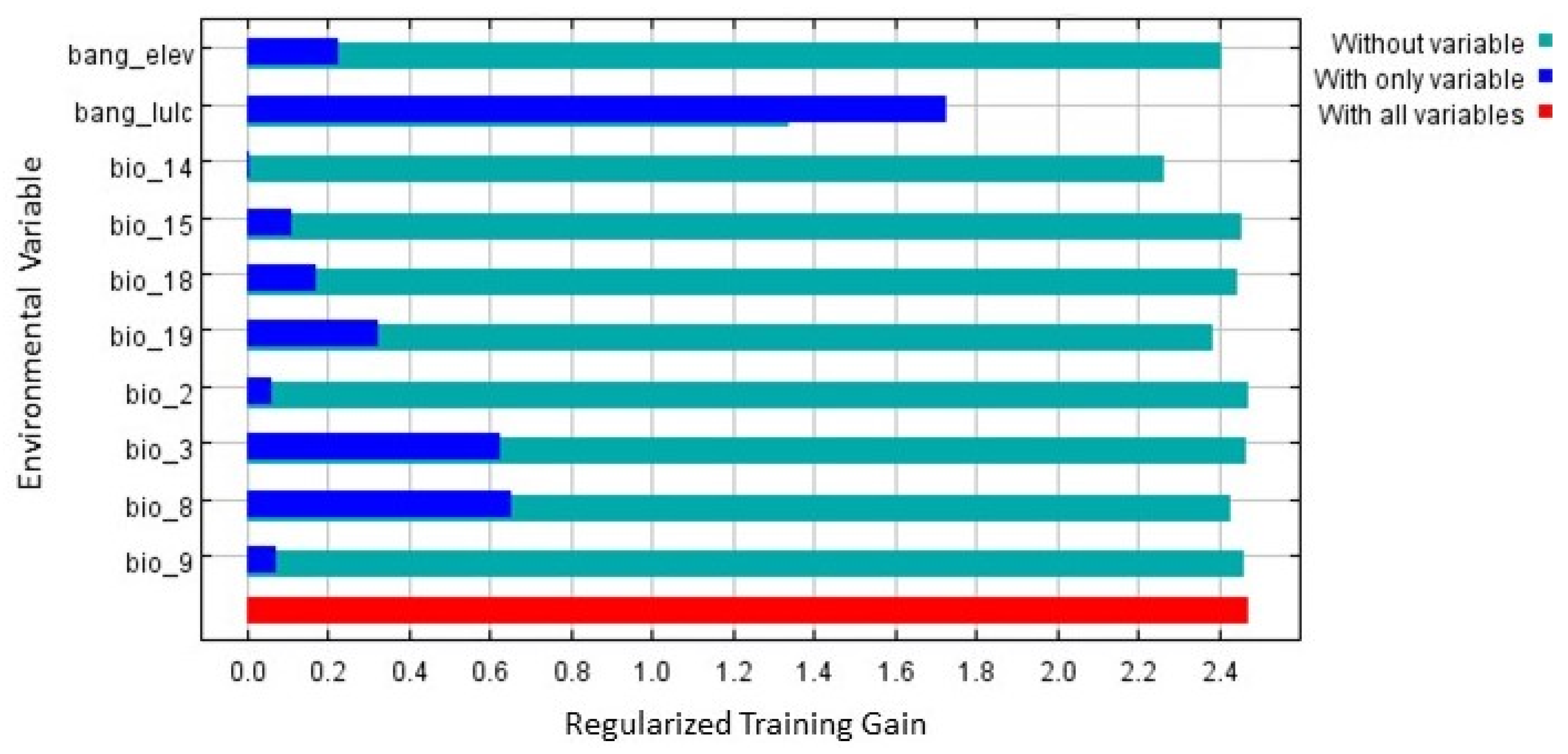
2.6. Modeling Procedures

We used MaxEnt 3.4.1 [27] for the modeling analyses. MaxEnt has been criticized because of its widespread use as a ‘blackbox’ tool using default settings [27,47,48,49,50,51,52]. We recognize that the use of default settings in MaxEnt could result in overfitting models that either oversimplify or complicate the output distribution, undermining the applicability of the model, especially with low occurrence data [47,48,50,51,52,53]. However, altering the settings based on recognized good practices for low sample size and associated model overfitting could result in useful distribution models [50,51,54]. The 10 environmental variables along with 12 presence records were used to run 15 replicates by the bootstrapping method. Replication averages model outcome thereby reducing skewness. Iterations were set to 5000 to aid in preventing the model from over or under-predicting the relationships considering the default recommended convergence threshold of 10−5. Random points were set to 10,000 points as the recommended default value. We selected linear and quadratic features based on the number of occurrences [47]. To further counteract model overfitting, several procedures were undertaken. Initially, our species locations had a good spatial distribution in the currently known habitat of the species. Since spatial resolution can also affect model fit and accuracy, we used a resolution of about 1 km for all our predictor variables. For conservation planning requirements, this resolution is considered adequate [48,49]. Further, according to two significant studies that investigated the effect of sample size on several SDMs using sample sizes ranging from very small to large sizes, MaxEnt mostly had the highest spatial conformity and accuracy, particularly for the smallest sample sizes of 5 and 10 [50]. In general, Maxent outperformed other modeling methods in producing beneficial results with small sample sizes [50,51]. Its algorithm, maximum entropy, was one of the least sensitive algorithms to sample size [51] and was found to remain within reasonable bounds in predicting the total area across all sample sizes [50]. Furthermore, the regularization in this algorithm is likely the key to avoid overfitting and compensate for small sample sizes [27,50]. This procedure helps MaxEnt assess the maximum entropy or the most uniform distribution across the investigated area, considering the constrains on the predicted distribution in that the average value for each environmental predictor is close, rather than equal, to the empirical average [27,50]. As a result, we tested the regularization parameter over a range of values and ultimately set it to 1 as higher values produced less accurate models with unsuitable areas while lower values resulted in overfit models. Finally, we set the random test percentage to zero since we tested the species distribution model (SDM) against a null model [52].

2.7. Evaluation of Model Performance

We assessed the accuracy of the model using the area under the receiving operator curve (AUC) value closer to 1 [53]. We also performed the null model approach [54] to assess if the AUC value deviates significantly from the null model AUC. We randomly sampled 12 localities without replacement from the 167,749 available cells of Bangladesh area using R and repeated the step 999 times. The random data was fed into MaxEnt to generate models under the same conditions as the species model to allow accurate comparison. The average AUC values of the null models were used to build a normal distribution histogram in R. We considered the model performance significantly better than random if the AUC of the species model was found greater than the upper limit of the 95% C.I. of AUC values [54,55].
We used Cohen’s kappa (k) [56] to further assess the model, with k < 0.4 representing poor accuracy, 0.4 < k < 0.75 representing good accuracy and k > 0.75 representing excellent accuracy [56]. We also calculated the true skill statistics (TSS) [57] to account for biases in accuracy with the kappa statistic [57,58]. Values ≤ 0 were considered random and +1 represented perfect model performance [59]. We used maximum training sensitivity and specificity threshold to perform the TSS and Cohen’s kappa tests [59]. Both measurements were conducted using R (ROCR, vcd and boot packages) and Microsoft Excel.

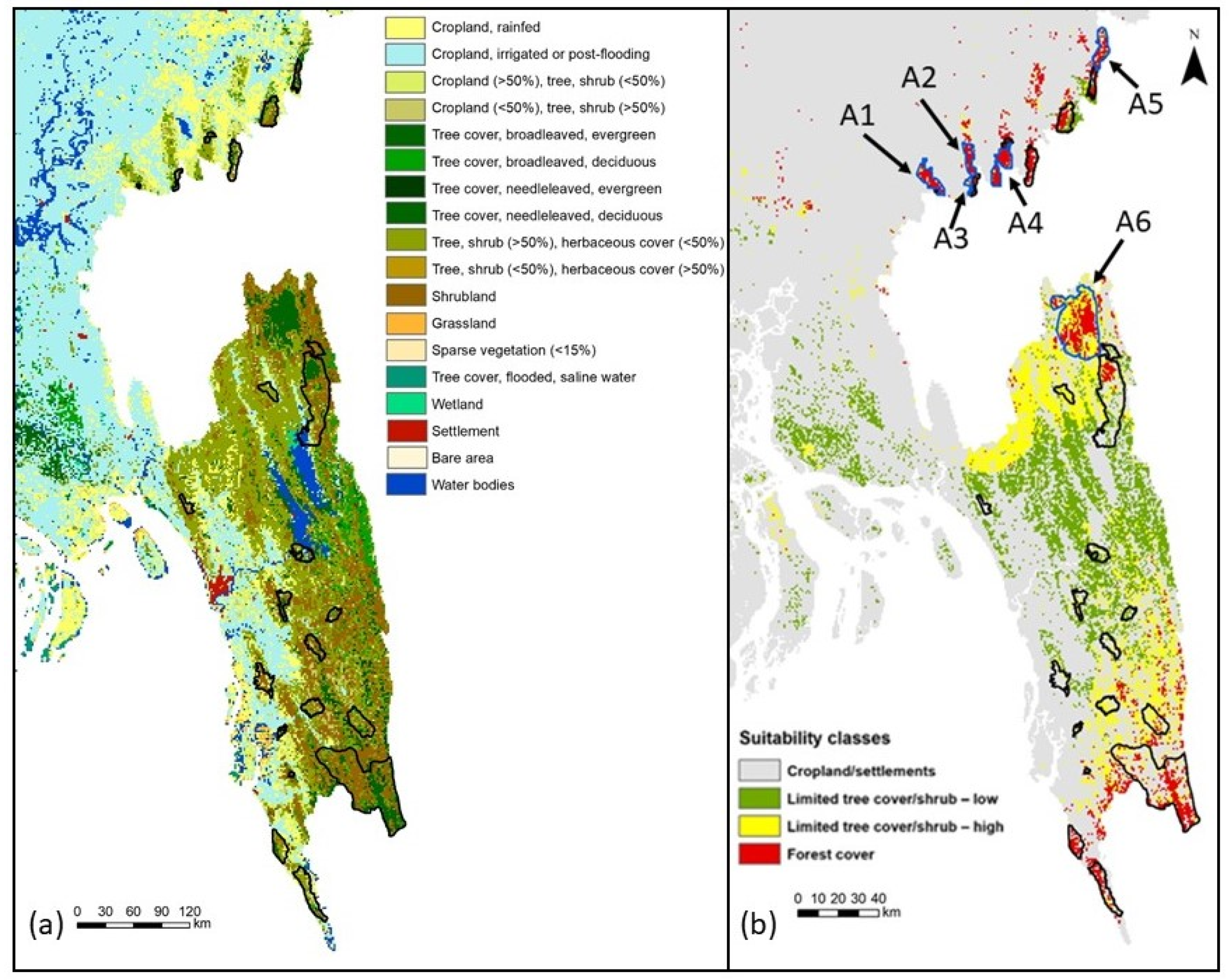
2.8. Habitat Suitability and Spatial Analysis

We classified the prediction produced by MaxEnt into four classes namely unsuitable (<0.1), least suitable (0.1−0.3), moderately suitable (0.3−0.6), and highly suitable (>0.6) [60]. We derived classification breaks using the Jenks Optimization method (i.e., Jenks Natural Breaks) [61] available in the spatial analyst tool in ArcGIS. By giving a certain number of classes, the method creates these natural breaks that are inherent in the data itself where it reduces the variance within classes and maximizes the variance between classes [61,62,63]. This classification method is markedly accurate, and boundaries do not change for each run [61]. Area calculation for the suitability classes were calculated using the same tool. Our initial assessment of the maps generated by MaxEnt in relation to LULC and elevation information extracted from Google Earth indicated that the areas classified as ‘unsuitable’ (color coded grey) in MaxEnt classified map corresponded to croplands or settled areas in LULC classifications; areas categorized as ‘least suitable’ (green) corresponded to limited tree cover/shrub in slightly high elevations; areas classified as ‘moderately suitable’ (yellow) corresponded to limited tree cover/shrub cover in low elevations; and areas classified as ‘highly suitable’ (red) were the only ones that overlapped with forest. We therefore replaced MaxEnt classified map categories with the following classification: grey (cropland/settlements), green (limited tree cover/shrub–high), yellow (limited tree cover/shrub–low, and red (forest cover). We highlighted areas of contiguous forest cover (red) outside of any of the protected areas visually. We then calculated the extent of forest cover from MaxEnt generated map to identify additional areas of conservation value for western hoolock gibbons in Bangladesh.

3. Results

3.1. Group Density and Population Estimates

A total of 109 days were spent conducting surveys of western hoolock gibbons on 76 transects (Mean 3.45±1.65 standard deviation per site, range 1–7), covering a distance of 204.65 km (Table 2). Mean density of groups was estimated to be 0.39 groups/km2 with group densities ranging between sites from 0.06–1.69 groups/km2 (Table 2). The Lawachara population was determined to be 40 individuals in 13 groups based on a total count, making the density of Lawachara to be 1.70 groups/km2. Density obtained from our Bayesian approach was 1.69 ± 0.67 groups/km2, suggesting that our density estimates were reasonable. The total number of western hoolock gibbon groups in Bangladesh was estimated to be 135.31 ± 2.23 (SE) groups with 468.96 ± 45.56 individuals from 12 sites (Table 2). Patharia (with about 25 groups) and Rajkandi (with about 34 groups) were the two northeastern sites with large numbers of western hoolock gibbons. In the southeastern regions, the number of groups was considerably lower, with Kaptai identified as a stronghold with an estimated 24 groups along with Sangu-Matamuhuri with about 21 groups. All remaining populations were low, or zero in numbers, consistent with the lack of suitable habitat at those sites.

3.2. Model Evaluation and Habitat Quality

The ROC curve for the western hoolock gibbon distribution showed a credible level of accuracy with an AUC of 0.989 and standard deviation of 0.003. The 95% C.I. AUC value of the randomly drawn null model was 0.879 (Table 3). Hence, the observed species distribution was significantly different from random. Cohen’s Kappa also showed that model accuracy falls in the good range where k max = 0.45 (0.4 < k < 0.75) [57]. The accuracy of the model performance was further supported by TSS, where the mean value was found equal to 0.907 and that reflects high performance. The relative importance of the predictor variables and their contribution to MaxEnt model were evaluated using Jackknife test results (Figure 2). LULC had the highest model gain when used in isolation. It is also the variable that decreased the model gain when omitted. Thus, the variable appeared to have the most information that was absent in the other variables. To be specific, forest types of broadleaved evergreen trees, broadleaved deciduous trees and mosaics of tree and shrub areas were collectively the most crucial as found in the variable response curve. Mean temperature of wettest quarter/season (Bio8) came second where habitat suitability remained high in temperatures above 27.5 °C. Followed closely by isothermality (a quantitative estimate of how large the day-to-night temperatures oscillate relative to the summer-to-winter (annual) oscillations) where high suitability was found at 45.8% and above. Therefore, the distribution of suitable habitats may be influenced by larger temperature fluctuations within a month relative to the year. Precipitation of the coldest quarter (Bio19) also showed high probability of Hoolock gibbon distribution when the value was ≥40mm. Similarly, habitat suitability was high when the elevation was ≥50m; however, suitability stabilized beyond 450m.
Approximately 14.95% representing an area of 294.54 km2 of the areas surveyed was highly suitable for western hoolock gibbons (Table 2, Figure 3). The MaxEnt model predicted that approximately 1.4% of Bangladesh representing a total area of 1878 km2 consistent with suitable forest cover for western hoolock gibbons. Thus, an additional 1583.46 km2 could potentially be available that require additional survey to determine the occurrence of western hoolock gibbons. Rajkandhi and Atora Hill in the northeast and Sangu-Matamuhuri, Pablakhali, Inani and Teknaf had highly suitable habitat. Furthermore, Satchari, Rema-KalengaandPatharia Hill had substantial forest stands north of them while Lawachara NP had substantial areas mostly on its southwest. In the northeast, MaxEnt classified model identified five areas (identified as A1–A5) with suitable tree cover and bioclimatic variables for western hoolock gibbons ranging from 33 to 61 km2 in area (Table 4, Figure 3). In the southeast, the MaxEnt model identified a large area of suitable forest cover for western hoolock gibbons northwest of Sajek Valley and Pablakhali totaling to about 244 km2 (area A6, Table 4, Figure 3). Thus, the model was able to identify a total area of about 492.76 km2 of forest cover suitable for gibbons. Group density was not significantly related to habitat quality, but was significantly related to protected status (One Way ANOVA, F = 6.92, p = 0.01), with national parks, wildlife sanctuaries and reserve forests having significantly more western hoolock gibbon populations compared to those that were not under official protection.

4. Discussion

Gibbons around the world face innumerable challenges from deforestation and resultant habitat loss [9,10,11,12,20]. The problems of deforestation in Bangladesh are acute, with very little forest remaining in patches in the northeast, southeast and central portions of the country, with the Sundarbans mangrove forests in the southwest being an exception [3,4,8]. Our current estimate covered many of the sites studied earlier, although we excluded the ones that were known to have no western hoolock gibbons due to loss of forest cover since the time the previous studies were undertaken [6,8].
The estimated mean group density of 0.39 groups/km2 was considerably lower than most group densities estimated for western hoolock gibbons in other areas or for other gibbon species in Southeast Asia. For example, Choudhury [64] estimated group density in 2004 across 10 large forest fragments and 35 small, isolated sites within the Karbi Anglong district of Assam. Although his estimates were crude, mean density was 0.76 groups/km2 with a range of 0.19–1.76 groups/km2 (group estimates calculated from individuals/km2 provided in Choudhury [64]). Das et al. [65] estimated a mean density of 0.2 groups/km2 covering the entire distribution of the western hoolock gibbon in India. He attributed the lower estimates of group density to severely degraded forest habitats, level of isolation of forest patches and poaching activities in many of the sites in northeastern India [66,67]. Other independent estimates of western hoolock gibbons in Namdapha in northeastern India suggested a density of 0.74 groups/km2 [67].
Generally, auditory methods appear to overestimate gibbon densities [26,68]. For example, estimates of 1.41–2.60 groups/km2 of western hoolock gibbons have been obtained from Namdapha [67]. Cheyne et al. [26] found that group densities of Bornean agile gibbons (Hylobates albibarbis), Muller’s gray gibbons (H. mulleri) and northern gray gibbons (H. funereus) ranged between 1.08–3.18 groups/km2 across many sites in Indonesian Borneo. In comparison, density of the red-cheeked gibbons (Nomascusgabriellae) estimated in a conservation area in Cambodia using the transect method was 0.73 ± 0.22 groups/km2 [25]. Density estimates of the critically endangered northern white-cheeked gibbon (Nomascus leucogenys) ranged from 0.4–0.7 groups/km2 [67]. Gibbon densities of 5–6 groups/km2 are considered to be high, whereas densities less than 2 groups/km2 are considered to be low [69]. Our estimates of group density were considerably lower than 2 groups/km2 in all the sites and were comparable to the densities of western hoolock gibbon populations in India as well as other critically endangered gibbon species. Furthermore, our estimates of density were consistent with the relatively poor quality of habitats that consist of severely degraded, isolated forests [4]. Thus, habitat quality is likely to be one of the prime factors influencing gibbon density in Bangladesh [6].
Sarma et al. [34] estimated the distribution of eastern hoolock gibbons in Arunachal Pradesh, India using normalized difference vegetation index (NDVI) layers along with LULC layers in MaxEnt. They used the same bioclimatic variables as in our study and found that precipitation of the coldest quarter contributed significantly towards the model, along with major contributions attributed to NDVI [34]. In our study, isothermality and mean temperature in the wettest quarter contributed substantially towards the model. We suggest that differences in the environmental variables in Sarma et al. [34] and our study is reflective of differences in the niches of these two species, an area that needs further study. The contribution of LULC in our model and NVDI in Sarma et al. [34] highlighted the importance of dense vegetation in determining distribution of both these gibbon species. Alamgir et al. [35] modelled the western hoolock gibbon population distribution in Bangladesh and found that isothermality, annual precipitation, elevation and mean temperature of the warmest quarter contributed substantially towards their distribution. This was largely consistent with our study with one exception: annual precipitation was excluded from the model during preprocessing. The exclusion of annual precipitation could be due to changes in environmental variables relating to precipitation already predicted in Alamgir et al. [35]. Similarly, Sarma et al. [36] found that vegetational factors were strongly influenced distribution of western hoolock gibbons in Assam. They used finer scale analysis that was able to highlight the importance of closed canopy forests for western hoolock gibbons. However, they also found that the mean temperature at the coldest quarter of the year influenced distribution, suggesting that food availability could be impacted by this environmental variable. Our model suggests that fine scale differences in environmental variables, particularly precipitation [35] or temperature patterns [36], need to be carefully evaluated to better understand the long-term changes in the habitat and therefore distribution of the western hoolock gibbon in Bangladesh and elsewhere.
Our estimate of populations in Rajkandi and Patharia Hill was expected since both the MaxEnt model and our own ground truthing indicated good forest cover suitable for western hoolock gibbons. The historical significance of Lawachara is withheld as it has maintained populations of about 30–42 individuals in 9–13 groups since the 1990s [7,24]. Generally, southeastern sites had significantly less gibbons since the previous surveys [6,7,18,20,70,71]. Of the southeastern sites, Sangu-Matamuhuri appears to have large forest tracts and we believe that the difficulties (political unrest and safety concerns) of surveying this area led to low encounter rates in our study. Islam et al. [7] reported one group with two individuals, although the survey covered a small area. Our estimate of about 76 individuals in 21 groups is a noted addition to the western hoolock gibbon population of Bangladesh. Furthermore, the population of Kaptai was reported to be 84 individuals in Islam et al. (2008) and our estimate of 86 individuals in 24 groups suggests a stable population. The areas north of Pablakhali Wildlife Sanctuary highlighted by the MaxEnt model is part of the Kassalong Reserve Forest [70] and it holds significant potential for hoolock gibbons. Tourism and development in the region has increased, along with a steady decline in forest cover [4], making this population vulnerable to declines in the future. Nevertheless, our study highlights Rajkandi, Patharia and some adjoining areas in the northeast; and Sangu-Matamuhuri, Kaptai and some areas north of Pablakhali in the southeast of Bangladesh as priority areas for conservation action for the species.
We also suggest that the population of western hoolock gibbons in Bangladesh is likely higher than what we have estimated, since many areas with potential western hoolock gibbon habitat were identified using our MaxEnt model. The identification of suitable habitats both in the northeast and southeast of Bangladesh allows for significant planning for conservation of this endangered primate. The MaxEnt model identified a total of over 1500 km2 of additional habitat suitable for western hoolock gibbons. However, many of these habitats were isolated patches. Of these sites with suitable habitats, the areas outside of the surveyed sites in the northeast collectively could add at least 120 km2 suitable for western hoolock gibbons. Furthermore, a large patch of suitable habitat was detected in the northern end of Pablakhali representing at least 70 km2. Although no encounters were made in Pablakhali, the area could serve as a potential reintroduction site if small, isolated populations that are not genetically viable were located in smaller, poorer quality habitat. The areas within and surrounding Kassalong Reserve Forest [70] located northwest of Sajek Valley and Pablakhali, representing at least 130 km2 consists of suitable habitat, was not been surveyed in this study and the density of western hoolock gibbons in these areas needs to be determined. Thus, survey and population assessment must be intensified in all sites with more than 30 individuals (Rajkandi, Patharia, Kaptai, and Sangu-matamuhuri) and the prospective sites with high quality habitat identified by MaxEnt modeling as highly suitable for western hoolock gibbons.
Bangladesh has at least 37 protected areas categorized as wildlife sanctuaries, national parks, or community conserved areas that face innumerable threats [3,8]. Management has been historically difficult with illegal activities abounding within the protected areas [3,8]. Nevertheless, the presence of forest guards and other staff at these locations has a negative effect on illegal activities depending on the location of the protected area and accessibility to humans [3]. We showed that protected areas had significantly higher densities of western hoolock gibbons compared to those with no protection. This association between protected status and population size indicated that even with questionable protection, these areas fared better for western hoolock gibbons compared to unprotected areas. Illegal deforestation and the collection of forest products can have negative effects on wildlife [3,8]. However, at sites such as Lawachara, Satchari and a few other northeastern sites, there has been a decline in illegal activities [3]. The southeastern sites, however, have generally suffered more and declines in forest cover have been greater [4]. Overall, the declines in forest cover and concomitant loss of western hoolock gibbons recorded in this study is especially clear in unprotected as well as protected areas in the southeast [7]. Nevertheless, the link between protected status and western hoolock gibbon abundance is encouraging and we suggest a thorough review of the tools in protected areas management [3] to strengthen the existing protected areas network. Specifically for western hoolock gibbons that are captured for meat and for the wildlife trade [21,22], protection measures in the existing protected areas should be increased. Furthermore, we suggest addition of sites under official protection using evidence from this and other studies (e.g., Ahsan et al. [3]). Western hoolock gibbons may continue to persist if given a chance, as long as suitable forest cover is available. Therefore, identified suitable habitats need to be evaluated, surveyed for gibbons, restored if needed and brought under protection.

Author Contributions

Conceptualization, S.B.M. and H.N.; methodology, S.B.M.; software, A.J. and S.B.M.; formal analysis, H.N., H.A.-R., T.A., S.H., A.J., S.B.M.; investigation and field work H.N., H.A.-R., T.A., S.H., S.B.M.; resources, H.N. and S.B.M.; data curation, H.A.-R., T.A. and S.H.; writing—original draft preparation, S.B.M.; writing—review and editing, H.N., H.A.-R., T.A., S.H., A.J., S.B.M.; visualization, T.A. and A.J.; supervision, H.N., H.A.-R. and S.B.M.; project administration, H.N., H.A.-R.; funding acquisition, H.N., H.A.-R. and S.B.M. All authors have read and agreed to the published version of the manuscript.

Funding

This research was funded by U.S. Fish and Wildlife Service Great Ape Conservation Fund, grant number F19AP00130.

Institutional Review Board Statement

The work was done with ethical approval from the Forest Department of Bangladesh.

Informed Consent Statement

Not applicable.

Data Availability Statement

No new data were created or analyzed in this study. Data sharing is not applicable to this article.

Acknowledgments

We thank the Forest Department of Bangladesh for providing the necessary approvals and permits. We also thank the Department of Zoology and the administration of Jagannath University, Bangladesh for permission to conduct this work. Authors are grateful to Shahriar Caesar Rahman and Creative Conservation Alliance team for facilitating a field survey in the southeastern region. We are also grateful to the Divisional Forest Officers of different forests and local forest officials, local field guides for their assistantship during field surveys.

Conflicts of Interest

The authors declare no conflict of interest.

References

  1. FAO. State of the World’s Forests 2016. Forests and Agriculture: Land-Use Challenges and Opportunities; Food and Agriculture Organization of the United Nations: Rome, Italy, 2016. [Google Scholar]
  2. Slik, J.F.; Franklin, J.; Arroyo-Rodríguez, V.; Field, R.; Aguilar, S.; Aguirre, N.; Ahumada, J.; Aiba, S.I.; Alves, L.F.; Anitha, K.; et al. Phylogenetic classification of the world’s tropical forests. Proc. Natl. Acad. Sci. USA 2018, 115, 1837–1842. [Google Scholar] [CrossRef] [Green Version]
  3. Ahsan, M.M.; Aziz, N.; Morshed, H.M. Assessment of Management Effectiveness of Protected Areas of Bangladesh. SRCWP Project; Bangladesh Forest Department: Dhaka, Bangladesh, 2016. [Google Scholar]
  4. Potapov, P.; Siddiqui, B.N.; Iqbal, Z.; Aziz, T.; Zzaman, B.; Islam, A.; Pickens, A.; Talero, Y.; Tyukavina, A.; Turubanova, S.; et al. Comprehensive monitoring of Bangladesh tree cover inside and outside of forests, 2000–2014. Environ. Res. Lett. 2017, 12, 104015. [Google Scholar] [CrossRef]
  5. Champion, H.G.; Seth, S.K. A Revised Survey of the Forest Types of India; Manager of Publications: Delhi, India, 1968. [Google Scholar]
  6. Muzaffar, S.B.; Islam, M.A.; Feeroz, M.M.; Kabir, M.; Begum, S.; Mahmud, M.S.; Hasan, M.K. Habitat characteristics of the endangered hoolock gibbons of Bangladesh: The role of plant species richness. Biotropica 2007, 39, 539–545. [Google Scholar] [CrossRef]
  7. Islam, M.A.; Feeroz, M.M.; Muzaffar, S.B.; Kabir, M.; Begum, S.; Hasan, K.; Mahmud, S.; Chakma, S. Population status and conservation of Hoolock Gibbons (Hoolock hoolock Harlan 1834) in Bangladesh. J. Bombay Nat. Hist. Soc. 2008, 105, 19–23. [Google Scholar]
  8. Muzaffar, S.B.; Islam, M.A.; Kabir, D.S.; Khan, M.H.; Ahmed, F.U.; Chowdhury, G.W.; Aziz, M.A.; Chakma, S.; Jahan, I. The endangered forests of Bangladesh: Why the process of implementation of the Convention on Biological Diversity is not working. Biod. Cons. 2011, 20, 1587–1601. [Google Scholar] [CrossRef]
  9. Chivers, D.J. The swinging singing apes: Fighting for food and family in far-east forests. In The Apes: Challenges for the 21st Century, Conference Proceedings; Sodaro, V., Sodaro, C., Eds.; Brookfield Zoo: Brookfield, IL, USA, 2001; pp. 1–28. [Google Scholar]
  10. Mittermeier, R.A.; Ratsimbazafy, J.; Rylands, A.B.; Williamson, L.; Oates, J.F.; Mbora, D.; Ganzhorn, J.U.; Rodríguez-Luna, E.; Palacios, E.; Heymann, E.W.; et al. Primates in peril: The world’s 25 most endangered primates, 2006–2008. Primate Cons. 2007, 22, 1–40. [Google Scholar] [CrossRef]
  11. Thinh, V.N.; Mootnick, A.R.; Geissmann, T.; Li, M.; Ziegler, T.; Agil, M.; Moisson, P.; Nadler, T.; Walter, L.; Roos, C. Mitochondrial evidence for multiple radiations in the evolutionary history of small apes. BMC Evol. Biol. 2010, 10, 1–13. Available online: http://www.biomedcentral.com/1471-2148/10/74 (accessed on 26 June 2021). [CrossRef] [Green Version]
  12. Schwitzer, C.; Mittermeier, R.A.; Rylands, A.B.; Chiozza, F.; Williamson, E.A.; Wallis, J.; Cotton, A. Primates in Peril: The World’s 25 Most Endangered Primates 2014–2016; IUCN SSC Primate Specialist Group (PSG): London, UK; International Primatological Society (IPS): Chicago, IL, USA; Conservation International (CI): Virginia, VA, USA; Bristol Zoological Society: Bristol, UK, 2015. [Google Scholar]
  13. McConkey, K.R.; O’Farrill, G. Loss of seed dispersal before the loss of seed dispersers. Biol. Conserv. 2016, 201, 38–49. [Google Scholar] [CrossRef]
  14. McConkey, K.R. Seed dispersal by primates in Asian habitats: From species, to communities, to conservation. Int. J. Primatol. 2018, 39, 466–492. [Google Scholar] [CrossRef]
  15. Geissmann, T.; Grindley, M.E.; Lwin, N.; Aung, S.S.; Aung, T.N.; Htoo, S.B.; Momberg, F. The Conservation Status of Hoolock Gibbons in Myanmar; Gibbon Conservation Alliance: Zurich, Switzerland, 2013. [Google Scholar]
  16. Fan, P.F.; He, K.; Chen, X.; Ortiz, A.; Zhang, B.; Zhao, C.; Li, Y.Q.; Zhang, H.B.; Kimock, C.; Wang, W.Z.; et al. Description of a new species of Hoolock gibbon (Primates: Hylobatidae) based on integrative taxonomy. Am. J. Primatol. 2017, 79, e22631. [Google Scholar] [CrossRef] [PubMed]
  17. Fan, P.F.; Turvey, S.T.; Bryant, J.V. Hoolock tianxing (amended version of 2019 assessment). IUCN Red List. Threat. Species 2020, e.T118355648A166597159. Available online: https://dx.doi.org/10.2305/IUCN.UK.2020-1.RLTS.T118355648A166597159.en (accessed on 21 June 2021). [CrossRef] [Green Version]
  18. Molur, S.; Walker, S.; Islam, A.; Miller, P.; Srinivasulu, C.; Nameer, P.O.; Daniel, B.A.; Ravikumar, L. Conservation of Western Hoolock Gibbon (Hoolock hoolock hoolock) in India and Bangladesh: Population and Habitat Viability Assessment (PHVA) Workshop Report; Coimbatore, Zoo Outreach Organization/CBSG-South Asia: Coimbatore, India, 2005. [Google Scholar]
  19. IUCN Bangladesh. Red List of Bangladesh Volume 1: Summary; IUCN (International Union for Conservation of Nature), Bangladesh Country Office: Dhaka, Bangladesh, 2015. [Google Scholar]
  20. Molur, S.; Brandon–Jones, D.; Dittus, W.; Eudey, A.; Kumar, A.; Singh, M.; Feeroz, M.M.; Chalise, M.; Priya, P.; Walker, S. Status of South. Asian Primates: Conservation Assessment and Management Plan. (C.A.M.P.) Workshop Report; Zoo Outreach Organization: Tamil Nadu, India; CBSG-South Asia: Coimbatore, India, 2003. [Google Scholar]
  21. Alliance, C.C. A Preliminary Wildlife Survey in Sangu-Matamuhuri Reserve Forest, Chittagong Hill Tracts, Bangladesh; Unpublished report submitted to Bangladesh Forest Department: Dhaka, Bangladesh, 2016; p. 52. [Google Scholar]
  22. Gittins, S.P.; Akonda, A.W. What survives in Bangladesh? Oryx 1982, 16, 275–282. [Google Scholar] [CrossRef]
  23. Feeroz, M.M.; Islam, M.A. Ecology and Behaviour of Hoolock Gibbons of Bangladesh; Multidisciplinary Action Research Centre (MARC): Dhaka, Bangladesh, 1992; p. 76. [Google Scholar]
  24. Das, J.; Feeroz, M.M.; Islam, M.A.; Biswas, J.; Bujarborua, P.; Chetry, D.; Medhi, R.; Bose, J. Distribution of hoolock gibbon (Bunopithecus hoolock hoolock) in India and Bangladesh. Zoos’ Print J. 2003, 18, 969–976. [Google Scholar] [CrossRef]
  25. Rawson, B.M.; Clements, T.; Hor, N.M. Status and conservation of yellow-cheeked crested gibbons (Nomascusgabriellae) in the Seima Biodiversity Conservation Area, Mondulkiri Province, Cambodia. In The Gibbons; Springer: New York, NY, USA, 2009; pp. 387–408. [Google Scholar] [CrossRef]
  26. Cheyne, S.M.; Gilhooly, L.J.; Hamard, M.C.; Höing, A.; Houlihan, P.R.; Loken, B.; Phillips, A.; Rayadin, Y.; Capilla, B.R.; Rowland, D.; et al. Population mapping of gibbons in Kalimantan, Indonesia: Correlates of gibbon density and vegetation across the species’ range. Endang. Spec. Res. 2016, 30, 133–143. [Google Scholar] [CrossRef] [Green Version]
  27. Phillips, S.J.; Dudík, M. Modeling of species distributions with Maxent: New extensions and a comprehensive evaluation. Ecography 2008, 31, 161–175. [Google Scholar] [CrossRef]
  28. Bradie, J.; Leung, B. A quantitative synthesis of the importance of variables used in MaxEnt species distribution models. J. Biogeog. 2017, 44, 1344–1361. [Google Scholar] [CrossRef]
  29. Rabelo, R.M.; Goncalves, J.R.; Silva, F.E.; Rocha, D.G.; Canale, G.R.; Bernardo, C.S.; Boubli, J.P. Predicted distribution and habitat loss for the endangered black-faced black spider monkey Ateles chamek in the Amazon. Oryx 2020, 54, 699–705. [Google Scholar] [CrossRef]
  30. Sales, L.P.; Ribeiro, B.R.; Pires, M.M.; Chapman, C.A.; Loyola, R. Recalculating route: Dispersal constraints will drive the redistribution of Amazon primates in the Anthropocene. Ecography 2019, 42, 1789–1801. [Google Scholar] [CrossRef] [Green Version]
  31. Campos, F.A.; Jack, K.M. A potential distribution model and conservation plan for the critically endangered Ecuadorian capuchin, Cebus albifronsaequatorialis. Int. J. Primatol. 2013, 34, 899–916. [Google Scholar] [CrossRef]
  32. Cavalcante, T.; de Souza Jesus, A.; Rabelo, R.M.; Messias, M.R.; Valsecchi, J.; Ferraz, D.; Gusmao, A.C.; da Silva, O.D.; Faria, L.; Barnett, A.A. Niche overlap between two sympatric frugivorous Neotropical primates: Improving ecological niche models using closely-related taxa. Biod. Cons. 2020, 29, 2749–2763. [Google Scholar] [CrossRef]
  33. Moraes, B.; Razgour, O.; Souza-Alves, J.P.; Boubli, J.P.; Bezerra, B. Habitat suitability for primate conservation in north-east Brazil. Oryx 2020, 54, 803–813. [Google Scholar] [CrossRef]
  34. Sarma, K.; Kumar, A.; Krishna, M.; Medhi, M.; Tripathi, O.P. Predicting Suitable Habitats for the Vulnerable Eastern Hoolock Gibbon, Hoolock leuconedys, in India Using the MaxEnt Model. Folia Primatol. 2015, 86, 387–397. [Google Scholar] [CrossRef]
  35. Alamgir, M.; Mukul, S.A.; Turton, S.M. Modelling spatial distribution of critically endangered Asian elephant and Hoolock gibbon in Bangladesh forest ecosystems under a changing climate. Appl. Geogr. 2015, 60, 10–19. [Google Scholar] [CrossRef]
  36. Sarma, K.; Saikia, M.K.; Sarania, B.; Basumatary, H.; Baruah, S.S.; Saikia, B.P.; Kumar, A.; Saikia, P.K. Habitat monitoring and conservation prioritization of Western Hoolock Gibbon in upper Brahmaputra Valley, Assam, India. Sci. Rep. 2021, 11, 15427. [Google Scholar] [CrossRef]
  37. Stan Development Team. RStan: The R Interface to Stan. R Package Version 2.21.2. 2020. Available online: http://mc-stan.org/ (accessed on 11 August 2021).
  38. Jaynes, E.T. Probability Theory: The Logic. of Science; Cambridge University Press: Cambridge, UK, 2003. [Google Scholar]
  39. Sollmann, R.; Gardner, B.; Williams, K.A.; Gilbert, A.T.; Veit, R.R. A hierarchical distance sampling model to estimate abundance and covariate associations of species and communities. Methods Ecol. Evol. 2003, 7, 529–537. [Google Scholar] [CrossRef]
  40. ESA (European Space Agency). Oxfordshire. Available online: http://maps.elie.ucl.ac.be/CCI/viewer/download.php (accessed on 9 January 2021).
  41. ESRI (Environmental Systems Research Institute). ArcGIS Desktop; Release 10.8.1; Environmental Systems Research Institute: Redlands, CA, USA, 2020. [Google Scholar]
  42. Google Earth Pro 2017. Google Earth Pro Version 7.3. Available online: https://www.google.com/earth/download/gep/agree.html?hl=en-GB (accessed on 1 April 2021).
  43. Earth Point 2015. Earth point—Tools for Google Earth. Available online: http://www.earthpoint.us/Shapes.aspx (accessed on 10 September 2020).
  44. Hijmans, R.J.; Cameron, S.E.; Parra, J.L.; Jones, P.G.; Jarvis, A. Very high resolution interpolated climate surfaces for global land areas. Int. J. Climatol. A J. R. Meteorol. Soc. 2005, 25, 1965–1978. [Google Scholar] [CrossRef]
  45. NOAA National Centers for Environmental Information, U.S. Available online: https://www.ngdc.noaa.gov/mgg/topo/gltiles.html (accessed on 10 September 2020).
  46. Duque-Lazo, J.; Van Gils, H.; Groen, T.A.; Navarro-Cerrillo, R.M. Transferability of species distribution models: The case of Phytophthora cinnamomi in Southwest Spain and Southwest Australia. Ecol. Model. 2016, 320, 62–70. [Google Scholar] [CrossRef]
  47. Elith, J.; Graham, H.C.; Anderson, R.P.; Dudík, M.; Ferrier, S.; Guisan, A.; Hijmans, R.J.; Huettmann, F.; Leathwick, J.R.; Lehmann, A.; et al. Novel methods improve prediction of species’ distributions from occurrence data. Ecography 2006, 29, 129–151. [Google Scholar] [CrossRef] [Green Version]
  48. Guralnick, R.; Hill, A. Biodiversity informatics: Automated approaches for documenting global biodiversity patterns and processes. Bioinformatics 2009, 25, 421–428. [Google Scholar] [CrossRef] [PubMed]
  49. Robertson, M.P.; Cumming, G.S.; Erasmus, B.F.N. Getting the most out of atlas data. Divers. Distrib. 2010, 16, 363–375. [Google Scholar] [CrossRef]
  50. Hernandez, P.A.; Graham, C.H.; Master, L.L.; Albert, D.L. The effect of sample size and species characteristics on performance of different species distribution modeling methods. Ecography 2006, 29, 773–785. [Google Scholar] [CrossRef]
  51. Wisz, M.S.; Hijmans, R.J.; Elith, J.; Peterson, A.T.; Graham, C.H.; Guisan, A.; NCEAS Predicting Species Distributions Working Group. Effects of sample size on the performance of species distribution models. Divers. Distrib. 2008, 14, 763–773. [Google Scholar] [CrossRef]
  52. Raes, N.; terSteege, H. A null-model for significance testing of presence-only species distribution models. Ecography 2007, 30, 727–736. [Google Scholar] [CrossRef]
  53. Merckx, B.; Steyaert, M.; Vanreusel, A.; Vincx, M.; Vanaverbeke, J. Null models reveal preferential sampling, spatial autocorrelation and overfitting in habitat suitability modelling. Ecol. Model. 2011, 222, 588–597. [Google Scholar] [CrossRef] [Green Version]
  54. Fielding, A.H.; Bell, J.F. A review of methods for the assessment of prediction errors in conservation presence/absence models. Environ. Conserv. 1997, 24, 38–49. [Google Scholar] [CrossRef]
  55. Cohen, J. A coefficient of agreement for nominal scales. Educ. Psychol. Meas. 1960, 20, 37–46. [Google Scholar] [CrossRef]
  56. Landis, J.R.; Koch, G.G. An application of hierarchical kappa-type statistics in the assessment of majority agreement among multiple observers. Biometrics 1977, 33, 363–374. [Google Scholar] [CrossRef] [PubMed]
  57. Allouche, O.; Tsoar, A.; Kadmon, R. Assessing the accuracy of species distribution models: Prevalence, kappa and the true skill statistic (TSS). J. Appl. Ecol. 2006, 43, 1223–1232. [Google Scholar] [CrossRef]
  58. Lantz, C.A.; Nebenzahl, E. Behavior and interpretation of the κ statistic: Resolution of the two paradoxes. J. Clin. Epidemiol. 1996, 49, 431–434. [Google Scholar] [CrossRef]
  59. West, A.M.; Kumar, S.; Brown, C.S.; Stohlgren, T.J.; Bromberg, J. Field validation of an invasive species Maxent model. Ecol. Inf. 2016, 36, 126–134. [Google Scholar] [CrossRef] [Green Version]
  60. Chen, W.; Pourghasemi, H.R.; Kornejady, A.; Zhang, N. Landslide spatial modeling: Introducing new ensembles of ANN, MaxEnt, and SVM machine learning techniques. Geoderma 2017, 305, 314–327. [Google Scholar] [CrossRef]
  61. Jenks, G.F. The data model concept in statistical mapping. Int. Yearb. Cartogr. 1967, 7, 186–190. [Google Scholar]
  62. Gavazzi, G.M.; Madricardo, F.; Janowski, L.; Kruss, A.; Blondel, P.; Sigovini, M.; Foglini, F. Evaluation of seabed mapping methods for fine-scale classification of extremely shallow benthic habitats–application to the Venice Lagoon, Italy. Estuar. Coast. Shelf Sci. 2016, 170, 45–60. [Google Scholar] [CrossRef] [Green Version]
  63. Khan, F. An initial seed selection algorithm for k-means clustering of georeferenced data to improve replicability of cluster assignments for mapping application. Appl. Soft Comp. 2012, 12, 3698–3700. [Google Scholar] [CrossRef] [Green Version]
  64. Choudhury, A. The distribution, status and conservation of hoolock gibbon, Hoolock hoolock, in Karbi Anglong district, Assam, Northeast India. Primate Conserv. 2009, 24, 117–126. [Google Scholar] [CrossRef] [Green Version]
  65. Das, J.; Biswas, J.; Bhattacherjee, P.C.; Mohnot, S.M. The distribution and abundance of hoolock gibbons in India. In The Gibbons, Developments in Primatology: Progress and Prospects; Lappan, S., Whittaker, D.J., Eds.; Springer: New York, NY, USA, 2006. [Google Scholar] [CrossRef]
  66. Chetry, D.; Medhi, R.; Biswas, J.; Das, D.; Bhattacharjee, P.C. Nonhuman primates in the Namdapha national park, Arunachal Pradesh, India. Int. J. Primatol. 2003, 24, 383–388. [Google Scholar] [CrossRef]
  67. Ray, P.C.; Kumar, A.; Devi, A.; Krishna, M.C.; Khan, M.L.; Brockelman, W.Y. Habitat characteristics and their effects on the density of groups of western hoolock gibbon (Hoolock hoolock) in Namdapha National Park, Arunachal Pradesh, India. Int. J. Primatol. 2015, 36, 445–459. [Google Scholar] [CrossRef]
  68. Syxaiyakhamthor, K.; Ngoprasert, D.; Asensio, N.; Savini, T. Identifying priority areas for the conservation of the Critically Endangered northern white-cheeked gibbon Nomascusleucogenys in northern Lao. Oryx 2020, 54, 767–775. [Google Scholar] [CrossRef]
  69. Brockelman, W.Y.; Srikosamatara, S. Estimation of density of gibbon groups by use of loud songs. Am. J. Primatol. 1993, 29, 93–108. [Google Scholar] [CrossRef]
  70. De Milde, R.A.J.; Shaheduzzaman, M.; Chowdhury, J.A. The Kassalong and Rankhiang Reserved Forests in the Chittagong Hill Tracts; Bangladesh Forest Department: Dhaka, Bangladesh, 1985. [Google Scholar]
  71. Kabir, M.T.; Ahsan, M.F.; Cheyne, S.M.; Sah, S.A.M.; Lappan, S.; Bartlett, T.Q.; Ruppert, N. Population assessment of the endangered Western Hoolock Gibbon Hoolock hoolock Harlan, 1834 at Sheikh Jamal Inani National Park, Bangladesh, and conservation significance of this site for threatened wildlife species. J. Threat. Taxa 2021, 13, 18687–18694. [Google Scholar] [CrossRef]
Figure 1. Map showing the study sites in northeastern and southeastern Bangladesh. The areas consisted of closed canopy forest patches suitable for western hoolock gibbon that were surrounded by human habitation or farmlands. NP = National Park, WS=Wildlife Sanctuary, RF= Reserve Forest.
Diversity 13 00490 g001
Figure 2. Jackknife evaluation of the relative importance of the environmental variables and their contribution to the MaxEnt model.
Diversity 13 00490 g002
Figure 3. (a) Map showing forest distribution in eastern Bangladesh based on land-use/land-cover (version 2.1.1, ESA 2021) and (b) potential distribution of hoolock gibbons based on habitat quality (LULC), elevation and bioclimatic variables generated using MaxEnt modeling. The study sites are indicated with black outlines.
Diversity 13 00490 g003
Table 1. Variables included in the final Maxent model.
SymbolEnvironmental VariablesFinal Model
Elevation
LULCLand-use landcover
BIO1Annual Mean Temperature
BIO2Mean Diurnal Range
BIO3Isothermality
BIO4Temperature Seasonality
BIO5Max Temperature of Warmest Month
BIO6Min Temperature of Coldest Month
BIO7Temperature Annual Range
BIO8Mean Temperature of Wettest Quarter
BIO9Mean Temperature of Driest Quarter
BIO10Mean Temperature of Warmest Quarter
BIO11Mean Temperature of Coldest Quarter
BIO12Annual Precipitation
BIO13Precipitation of Wettest Month
BIO14Precipitation of Driest Month
BIO15Precipitation Seasonality
BIO16Precipitation of Wettest Quarter
BIO17Precipitation of Driest Quarter
BIO18Precipitation of Warmest Quarter
BIO19Precipitation of Coldest Quarter
Table 2. Estimated group density, total number of groups and individuals in populations of western hoolock gibbons in Bangladesh.
Site NameTotal Area of Sites (km2)Area LULC (Forest Area)MaxEnt (LULC + Elevation + Bioclim)Suitable Forest Cover (km2)Percentage Suitable Area (%)Number of TransectsTotal Transect Length (km)Number of Observed GroupsDensity of Groups (Groups/km2 ± 95% C.I.)Total Number of GroupsTotal Individuals
(±SE) d(±SE) d
1Satchari NP a2.4321.612.3596.7135.411.12 ± 0.982.62 ± 0.019.37 ± 1.00
2Lawachara NP12.61211.2510.0779.92711.7381.69 ± 0.461340
3Rema-KalengaWS b17.951214.4716.2690.58516.7900.0615
4RajkandhiRF c71.934449.0327.1437.73721.3541.27 ± 0.4834.33 ± 0.19122.57 ± 12.83
5Patharia RF36.822319.2921.6658.83518.5331.19 ± 0.5525.73 ± 0.1491.86 ± 9.55
6Atora Hill RF86.454641.889.2516.5100.1312
7Hazarikhil WS24.6212018.1973.88313.220000
8Dighinala40.213401.443.5836.170000
9Sajek Valley34.1901.484.34410.340000
10Pablakhali WS420.8718847.4369.0316.4036.90000
11Kaptai NP54.64291.6121.8940.06311.5421.11 ± 0.6524.23 ± 0.1386.51 ± 8.61
12Dhopachori-Dudhpukuria WS48.929015.5931.88415.70000
13Chimbuk55.53150.800.0048.80000
14Chunati WS77.156011.3814.7528.330000
15Bangdhepa4.6230.83.7781.5323.160000
16Bamu61.523001.943.15250000
17Fashiakhali WS12.93603.3125.5944.9921.19 ± 0.743.94 ± 0.0214.07 ± 1.59
18Innani RF74.294438.5839.753.4438.3500.05718
19Teknaf WS113.755345.028.587.5447.6600.1213
20Rowangchhari29.391505.5218.7836.860000
21Sangu-Matamuhuri RF803.67385247.58303.7347.3220.72 ± 0.5721.45 ± 0.1176.58 ± 6.72
22Thanchi102.715712.069.669.41000000
TOTAL 294.5414.95 135.31 ± 2.23468.96 ± 45.56
a NP; National Park, b WS; Wildlife Sanctuary, c RF: Reserve Forest, d numbers without decimals are actual groups and individuals in selected sites provided by forest officials and from Kabir et al. (2021) for Inani.
Table 3. Mean AUC a values of the species model and null models, TSS b and Kappa values for Hoolock hoolock distribution in Bangladesh.
Threshold IndependentThreshold Dependent
Study Model AUCStandard DeviationNull Models AUCOne Sided 95% C.I.TSSCohen’s Kappa (k) Max
0.9890.0030.8220.8790.9070.454
a Area Under the Curve, b True Skill Statistic.
Table 4. Areas identified to have suitable forest cover to support western hoolock gibbon populations based on MaxEnt modeling.
RegionForest Cover (km2)
Northeast
A1 (north of Satchari)61.09
A2 (north of Rema)49.03
A3 (east of Rema)33.76
A4 (south of Lawachara)52.25
A5 (north of Patharia)52.25
Southeast
A6 (northwest of Pablakhali)244.37
Total potential area492.76
Publisher’s Note: MDPI stays neutral with regard to jurisdictional claims in published maps and institutional affiliations.

