Coexistence of Two Closely Related Cyprinid Fishes (Hemiculter bleekeri and Hemiculter leucisculus) in the Upper Yangtze River, China

Abstract
1. Introduction
2. Materials and Methods
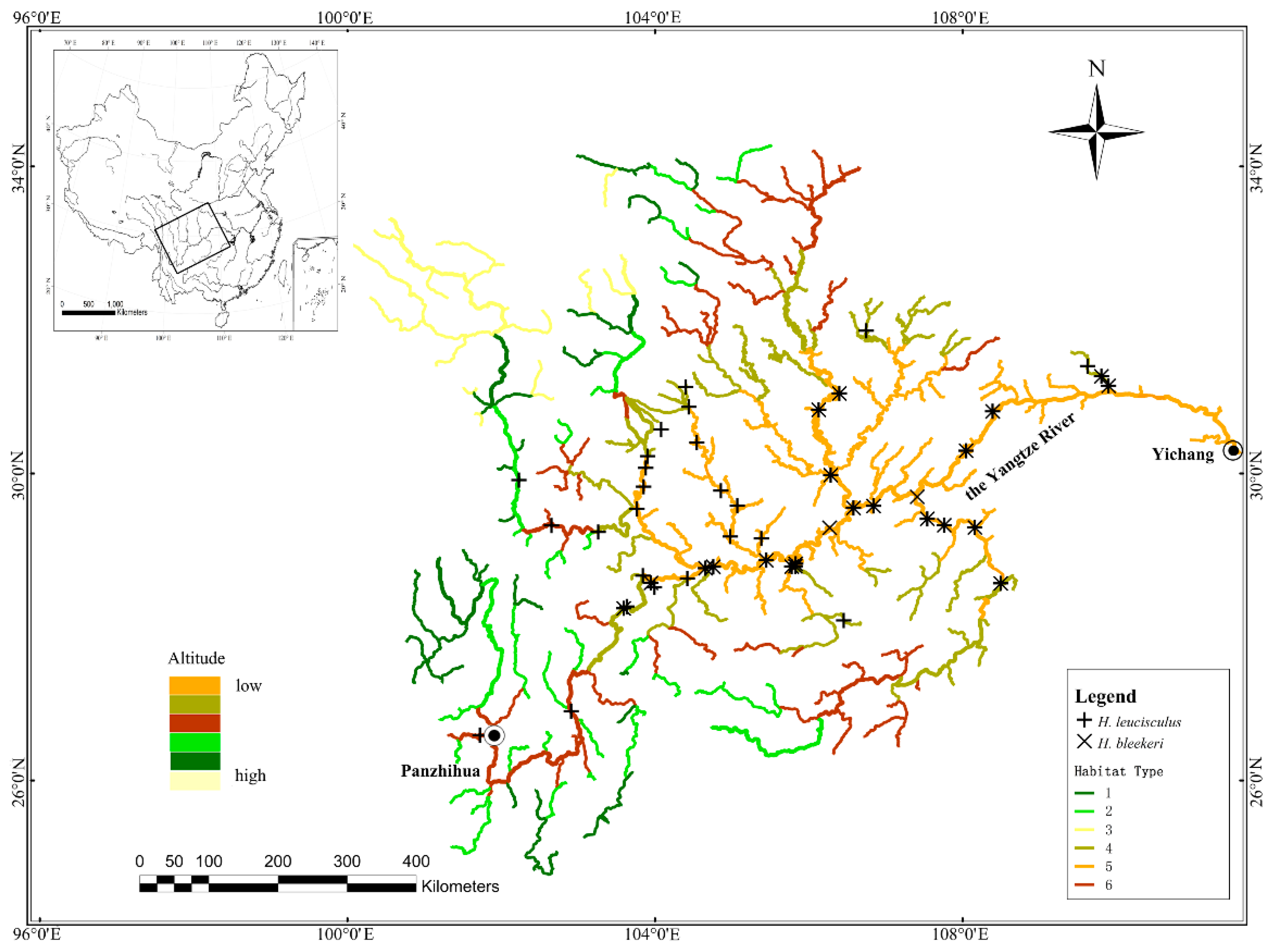
2.1. Study Area and Fish Sampling
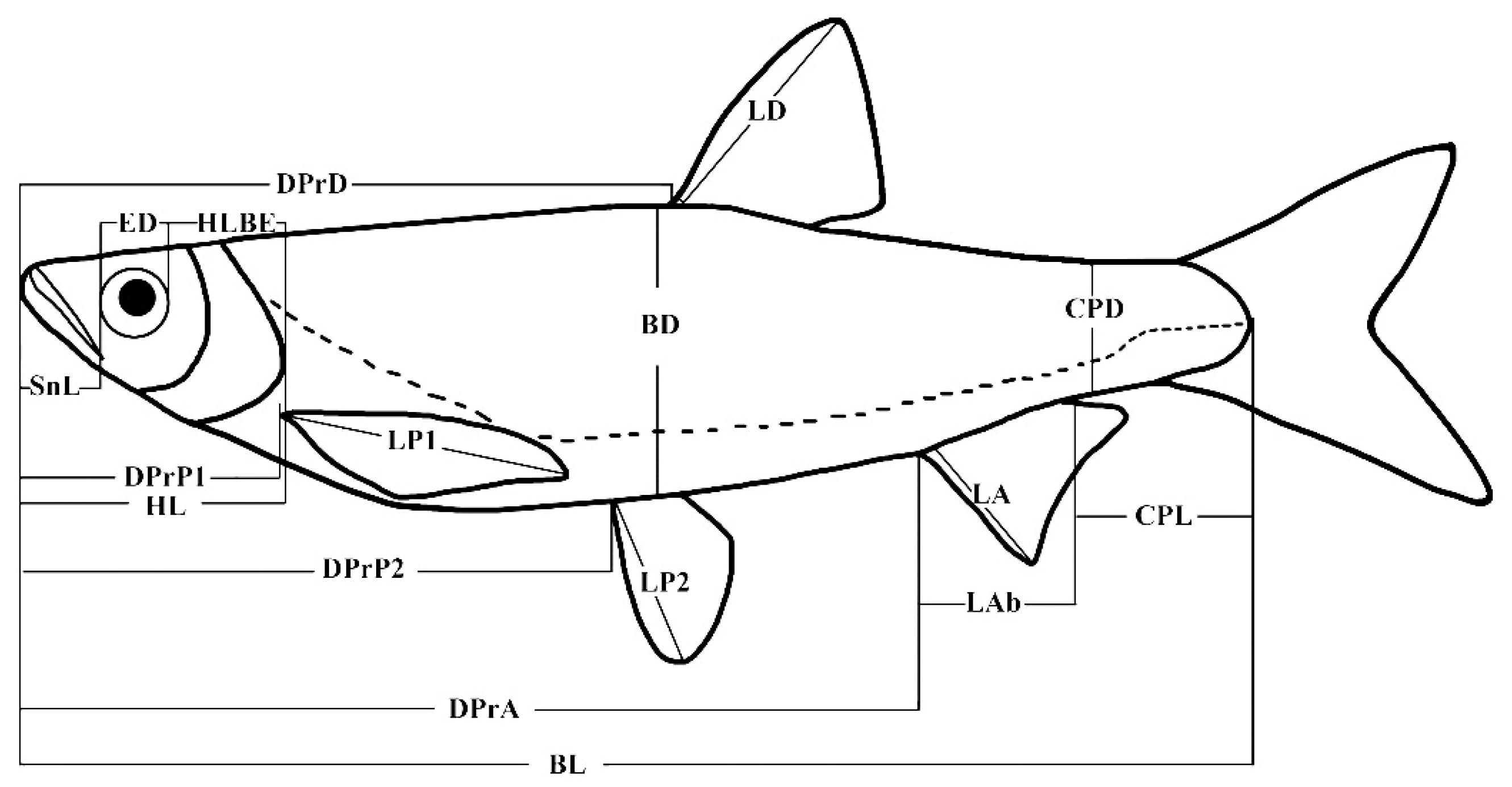
2.2. Morphological Measurement
2.3. Spatial Niche
2.3.1. Data Sources
2.3.2. Technical Procedure for Classifying River Habitats
2.3.3. Choice and Calculation of Habitat Classification Index
2.4. Trophic Niche
2.5. Statistical Analysis
3. Results
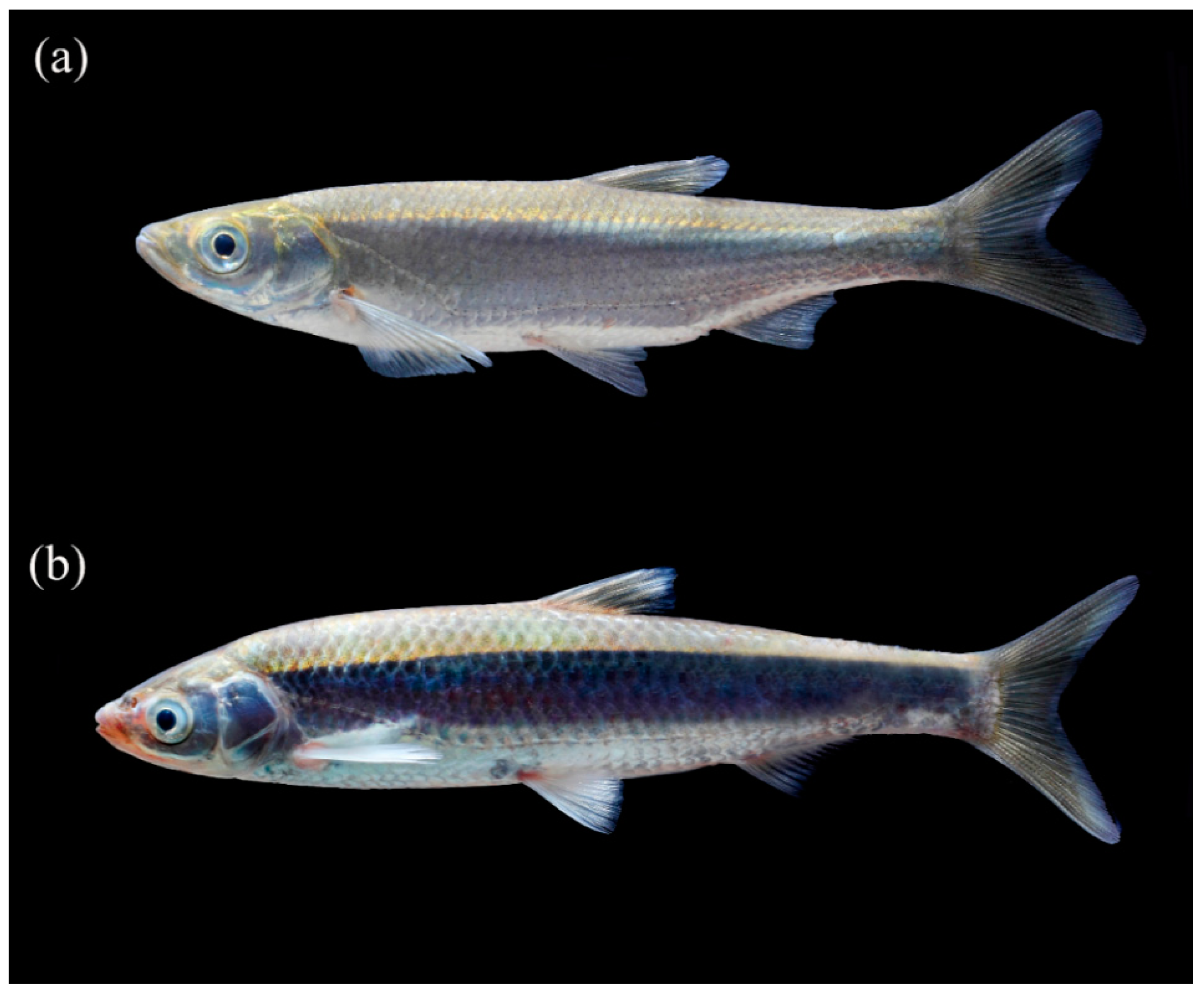
3.1. Morphological Measurements
3.2. Spatial Niche
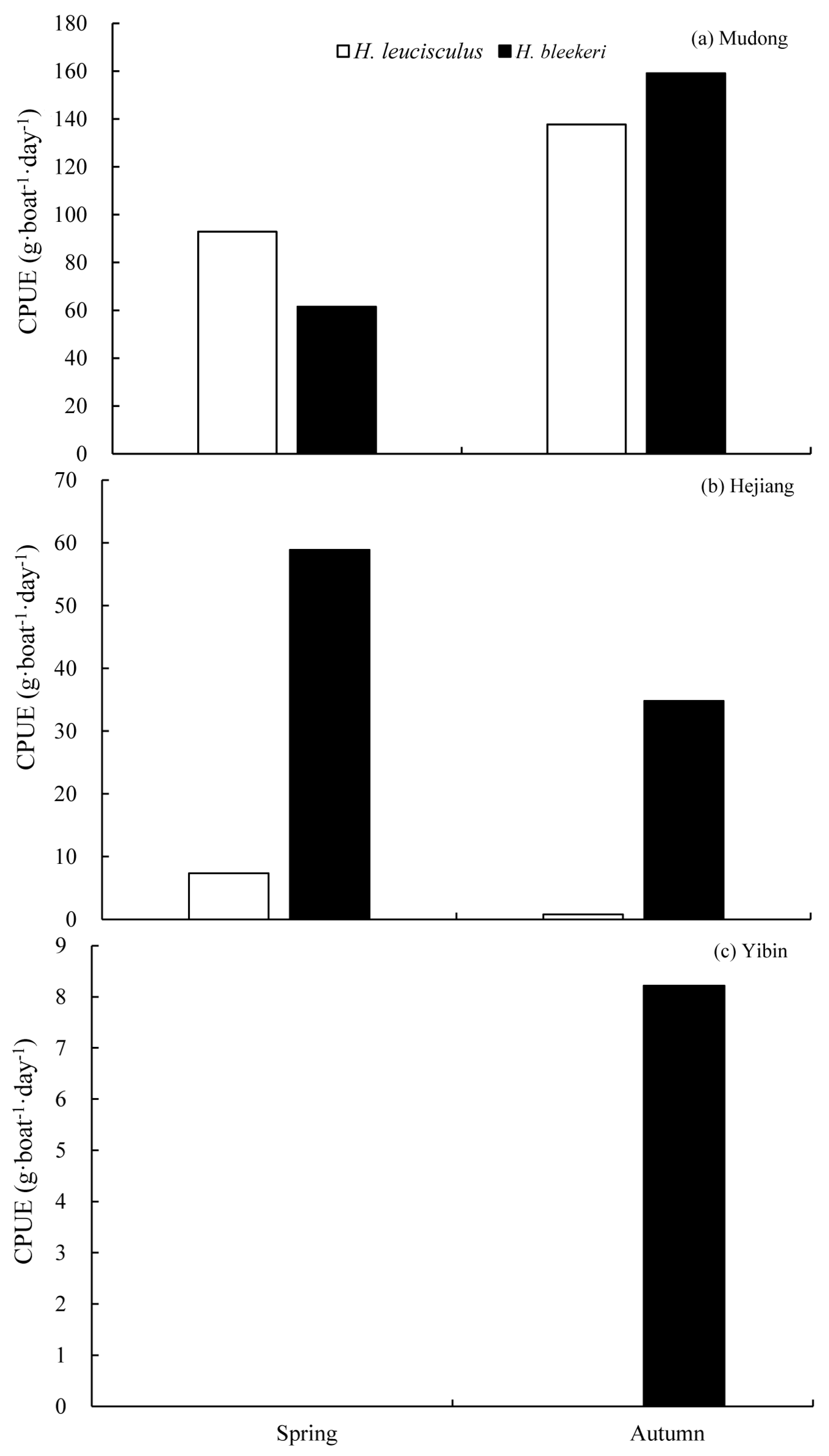
3.3. Temporal Niche
3.4. Trophic Niche
4. Discussion
4.1. Morphological Characteristics and Ecological Niches
4.2. Niche Segregation and Species Coexistence
5. Conclusions
Supplementary Materials
Author Contributions
Funding
Acknowledgments
Conflicts of Interest
References
- Carniatto, N.; Fugi, R.; Thomaz, S.M. Highly segregated trophic niche of two congeneric fish species in Neotropical floodplain lakes. J. Fish Biol. 2016, 90, 1118–1125. [Google Scholar] [CrossRef]
- Mouillot, D. Niche-assembly vs. dispersal-assembly rules in coastal fish metacommunities: Implications for management of biodiversity in brackish lagoons. J. Appl. Ecol. 2007, 44, 760–767. [Google Scholar] [CrossRef]
- Albrecht, M.; Gotelli, N.J. Spatial and temporal niche partitioning in grassland ants. Oecologia 2001, 126, 134–141. [Google Scholar] [CrossRef]
- Gause, G.F. The struggle for existence. Soil Sci. 1934, 41, 159. [Google Scholar] [CrossRef]
- Knickle, D.C.; Rose, G.A. Examination of fine-scale spatial-temporal overlap and segregation between two closely related congeners Gadus morhua and Gadus ogac in coastal Newfoundland. J. Fish Biol. 2014, 85, 713–735. [Google Scholar] [CrossRef]
- Knickle, D.C. Niche Partitioning in Sympatric Greenland Cod (Gadus ogac) and Atlantic Cod (Gadus morhua) in Coastal Newfoundland. Ph.D. Thesis, Memorial University of Newfoundland, St. John’s, NL, Canada, 2013. [Google Scholar]
- Neves, M.P.; Da Silva, J.C.; Baumgartner, D.; Baumgartner, G.; Delariva, R.L. Is resource partitioning the key? The role of intra-interspecific variation in coexistence among five small endemic fish species (Characidae) in subtropical rivers. J. Fish Biol. 2018, 93, 238–249. [Google Scholar] [CrossRef] [PubMed]
- Ross, S.T. Resource partitioning in fish assemblages: A review of field studies. Copeia 1986, 352–388. [Google Scholar] [CrossRef]
- Maci, S.; Basset, A. Composition, structural characteristics and temporal patterns of fish assemblages in non-tidal Mediterranean lagoons: A case study. Estuar. Coast. Shelf Sci. 2009, 83, 602–612. [Google Scholar] [CrossRef]
- Schoener, T.W. Resource partitioning in ecological communities. Science 1974, 185, 27–29. [Google Scholar] [CrossRef] [PubMed]
- Nagelkerken, I.; Velde, G.V.D.; Verberk, W.C.E.P.; Dorenbosch, M. Segregation along multiple resource axes in a tropical seagrass fish community. Mar. Ecol. Prog. Ser. 2006, 308, 79–89. [Google Scholar] [CrossRef]
- Randler, C.; Teichmann, C.; Pentzold, S. Breeding habitat preference and foraging of the Cyprus Wheatear Oenanthe cypriaca and niche partitioning in comparison with migrant Oenanthe species on Cyprus. J. Ornithol. 2010, 151, 113–121. [Google Scholar] [CrossRef]
- Richardson, M.L.; Hanks, L.M. Partitioning of niches among four species of orb-Weaving spiders in a grassland habitat. Environ. Entomol. 2009, 38, 651–656. [Google Scholar] [CrossRef] [PubMed]
- Hunt, D.E.; David, L.A.; Gevers, D.; Preheim, S.P.; Alm, E.J.; Polz, M.F. Resource partitioning and sympatric differentiation among closely related bacterioplankton. Science 2008, 320, 1081–1085. [Google Scholar] [CrossRef] [PubMed]
- Sampayo, E.M.; Franceschinis, L.; Hoegh-Guldberg, O.; Dove, S. Niche partitioning of closely related symbiotic dinoflagellates. Mol. Ecol. 2007, 16, 3721–3733. [Google Scholar] [CrossRef]
- Peterson, M.L.; Rice, K.J.; Sexton, J.P. Niche partitioning between close relatives suggests trade-offs between adaptation to local environments and competition. Ecol. Evol. 2013, 3, 512–522. [Google Scholar] [CrossRef] [PubMed]
- Silvertown, J. Plant coexistence and the niche. Trends Ecol. Evol. 2004, 19, 605–611. [Google Scholar] [CrossRef]
- Munday, P.L.; Jones, G.P.; Caley, M.J. Interspecific competition and coexistence in a guild of coral-dwelling fishes. Ecology 2001, 82, 2177–2189. [Google Scholar] [CrossRef]
- Silva, N.C.D.S.; Costa, A.J.L.d.; Louvise, J.; Soares, B.E.; Reis, V.C.E.S.; Albrecht, M.P.; Caramaschi, É.P. Resource partitioning and ecomorphological variation in two syntopic species of Lebiasinidae (Characiformes) in an Amazonian stream. Acta Amaz. 2016, 46, 25–36. [Google Scholar] [CrossRef]
- Cloyed, C.; Eason, P. Niche partitioning and the role of intraspecific niche variation in structuring a guild of generalist anurans. R. Soc. Open Sci. 2017, 4, 170060. [Google Scholar] [CrossRef]
- Lehtinen, R.M.; Glf, C. Habitat selection, the included niche, and coexistence in plant-specialist frogs from Madagascar. Biotropica 2011, 43, 58–67. [Google Scholar] [CrossRef]
- Rossier, O. Spatial and temporal separation of littoral zone fishes of Lake Geneva (Switzerland-France). Hydrobiologia 1995, 300–301, 321–327. [Google Scholar] [CrossRef]
- Leray, M.; Alldredge, A.L.; Yang, J.Y.; Meyer, C.P.; Holbrook, S.L.; Schmitt, R.J.; Knowlton, N.; Brooks, A.J. Dietary partitioning promotes the coexistence of planktivorous species on coral reefs. Mol. Ecol. 2019, 28, 2694–2710. [Google Scholar] [CrossRef]
- Peres-Neto, P.R. Alguns métodos e estudos em ecomorfologia de peixes de riachos. Oecologia Aust. 1999, 6. [Google Scholar] [CrossRef]
- Oliveira, E.F.; Goulart, E.; Breda, L.; Minte-Vera, C.V.; Paiva, L.R.D.S.; Vismara, M.R. Ecomorphological patterns of the fish assemblage in a tropical floodplain: Effects of trophic, spatial and phylogenetic structures. Neotrop. Ichthyol. 2010, 8, 569–586. [Google Scholar] [CrossRef]
- Sampaio, A.L.A.; Pagotto, J.P.A.; Goulart, E. Relationships between morphology, diet and spatial distribution: Testing the effects of intra and interspecific morphological variations on the patterns of resource use in two Neotropical Cichlids. Neotrop. Ichthyol. 2013, 11, 351–360. [Google Scholar] [CrossRef]
- Costa, C.; Cataudella, S. Relationship between shape and trophic ecology of selected species of Sparids of the Caprolace coastal lagoon (Central Tyrrhenian Sea). Environ. Biol. Fishes 2007, 78, 115–123. [Google Scholar] [CrossRef]
- Eklöv, P.; Svanbäck, R. Predation risk influences adaptive morphological variation in fish populations. Am. Nat. 2006, 167, 440–452. [Google Scholar] [CrossRef]
- Pakkasmaa, S.; Piironen, J. Water velocity shapes juvenile salmonids. Evol. Ecol. 2000, 14, 721–730. [Google Scholar] [CrossRef]
- Helland, I.P.; Vøllestad, L.A.; Freyhof, J.; Mehner, T. Morphological differences between two ecologically similar sympatric fishes. J. Fish Biol. 2009, 75, 2756–2767. [Google Scholar] [CrossRef]
- Svanbäck, R.; Eklöv, P.; Fransson, R.; Holmgren, K. Intraspecific competition drives multiple species resource polymorphism in fish communities. Oikos 2008, 117, 114–124. [Google Scholar] [CrossRef]
- Cochran-Biederman, J.L.; Winemiller, K.O. Relationships among habitat, ecomorphology and diets of cichlids in the Bladen River, Belize. Environ. Biol. Fishes 2010, 88, 143–152. [Google Scholar] [CrossRef]
- Gatz, A.J., Jr. Community organization in fishes as indicated by morphological features. Ecology 1979, 60, 711–718. [Google Scholar] [CrossRef]
- Leitão, R.P.; Sánchez-Botero, J.I.; Kasper, D.; Trivério-Cardoso, V.; Araújo, C.M.; Zuanon, J.; Caramaschi, É.P. Microhabitat segregation and fine ecomorphological dissimilarity between two closely phylogenetically related grazer fishes in an Atlantic Forest stream, Brazil. Environ. Biol. Fishes 2015, 98, 2009–2019. [Google Scholar] [CrossRef]
- Tan, X.; Li, X.; Lek, S.; Li, Y.F.; Wang, C.; Li, J.; Luo, J.R. Annual dynamics of the abundance of fish larvae and its relationship with hydrological variation in the Pearl River. Environ. Biol. Fishes 2010, 88, 217–225. [Google Scholar] [CrossRef]
- IHB (Institute of Hydrobiology). Fishes in the Yangtze River; Science Press: Beijing, China, 1976. (In Chinese) [Google Scholar]
- Bonato, K.O.; Burress, E.D.; Fialho, C.B.; Armbruster, J. Resource partitioning among syntopic Characidae corroborated by gut content and stable isotope analyses. Hydrobiologia 2017, 805, 1–14. [Google Scholar] [CrossRef]
- Mol, J.H. Ontogenetic diet shifts and diet overlap among three closely related Neotropical armoured catfishes. J. Fish Biol. 1995, 47, 788–807. [Google Scholar] [CrossRef]
- Mooney, K.A.; Jones, P.; Agrawal, A.A. Coexisting congeners: Demography, competition and interactions with cardenolides for two milkweed-feeding aphids. Oikos 2008, 117, 450–458. [Google Scholar] [CrossRef]
- He, Y.; Wang, J.; Lek-Ang, S.; Lek, S. Predicting assemblages and species richness of endemic fish in the upper Yangtze River. Sci. Total Environ. 2010, 408, 4211–4220. [Google Scholar] [CrossRef]
- Dong, Z.R. Diversity of river morphology and diversity of biocommunities. J. Hydraul. Eng. 2003, 11, 1–6. [Google Scholar] [CrossRef]
- Ding, R. The Fishes of Sichuan, China; Sichuan Publishing House of Science and Technology: Chengdu, China, 1994. (In Chinese) [Google Scholar]
- Wang, M.; Liu, F.; Lin, P.; Yang, S.; Liu, H. Evolutionary dynamics of ecological niche in three rhinogobio fishes from the upper Yangtze River inferred from morphological traits. Ecol. Evol. 2015, 5, 567–577. [Google Scholar] [CrossRef]
- Chen, Y.Y. (Ed.) Fauna Sinica—Osteichthyes Cyperiniformes II; Science Press: Beijing, China, 1998; pp. 225–228. [Google Scholar]
- Kai, Y.; Nakabo, T. Morphological differences among three color morphotypes of sebastes inermis (scorpaenidae). Ichthyol. Res. 2002, 49, 260–266. [Google Scholar] [CrossRef]
- Chuang, L.C.; Lin, Y.S.; Liang, S.H. Ecomorphological comparison and habitat preference of 2 cyprinid fishes, varicorhinus barbatulus and candidia barbatus, in Hapen Creek of Northern Taiwan. Zool. Stud. 2006, 45, 114–123. [Google Scholar]
- Motta, P.J.; Clifton, K.B.; Hernandez, P.; Eggold, B.T. Ecomorphological correlates in ten species of subtropical seagrass fishes: Diet and microhabitat utilization. Environ. Biol. Fishes 1995, 44, 37–60. [Google Scholar] [CrossRef]
- Kassam, D.D.; Adams, D.C.; Hori, M.; Yamaoka, K. Morphometric analysis on ecomorphologically equivalent cichlid species from Lakes Malawi and Tanganyika. J. Zool. 2002, 260, 153–157. [Google Scholar] [CrossRef]
- Kong, W.; Sun, O.J.; Chen, Y.; Yu, Y.; Tian, Z. Patch-level based vegetation change and environmental drivers in Tarim River drainage area of West China. Landscape Ecol. 2010, 25, 1447–1455. [Google Scholar] [CrossRef]
- Higgins, J.V.; Bryer, M.T.; Khoury, M.L.; Fitzhugh, T.W. A freshwater classification approach for biodiversity conservation planning. Conserv. Biol. 2005, 19, 432–445. [Google Scholar] [CrossRef]
- Cohen, S.; Wan, T.; Islam, M.T.; Syvitski, J.P.M. Global river slope: A new geospatial dataset and global- scale analysis. J. Hydrol. 2018, 563, 1057–1067. [Google Scholar] [CrossRef]
- Allan, J.D.; Castillo, M.M. Stream Ecology: STRUCTURE and Function of Running Waters, 2nd ed.; Springer: Dordrecht, The Netherlands, 2007; pp. 1–436. [Google Scholar] [CrossRef]
- Yao, X.Y.; Huang, G.T.; Xie, P.; Xu, J. Trophic niche differences between coexisting omnivores silver carp and bighead carp in a pelagic food web. Ecol. Res. 2016, 31, 831–839. [Google Scholar] [CrossRef]
- Lahnsteiner, F.; Jagsch, A. Changes in phenotype and genotype of Austrian Salmo trutta populations during the last century. Environ. Biol. Fishes 2005, 74, 51–65. [Google Scholar] [CrossRef]
- Brosse, S.; Giraudel, J.; Lek, S. Utilisation of non-supervised neural networks and principal component analysis to study fish assemblages. Ecol. Model. 2001, 146, 159–166. [Google Scholar] [CrossRef]
- Samaee, S.M.; Mansour, N. Morphological differentiation within the population of Siah Mahi, Capoeta capoeta gracilis, (Cyprinidae, Teleostei) in a river of the south Caspian Sea basin: A pilot study. J. Appl. Ichthyol. 2009, 25, 583–590. [Google Scholar] [CrossRef]
- Kaiser, H.F. The application of electronic computers to factor analysis. Educ. Psychol. Meas. 1960, 20, 141–151. [Google Scholar] [CrossRef]
- Gao, X.; Zeng, Y.; Wang, J.; Liu, H. Immediate impacts of the second impoundment on fish communities in the three gorges reservoir. Environ. Biol. Fishes 2010, 87, 163–173. [Google Scholar] [CrossRef]
- Jackson, A.L.; Inger, R.; Parnell, A.C.; Bearhop, S. Comparing isotopic niche widths among and within communities: SIBER—Stable Isotope Bayesian Ellipses in R. J. Anim. Ecol. 2011, 80, 595–602. [Google Scholar] [CrossRef]
- Jackson, M.C.; Donohue, I.; Jackson, A.L.; Britton, J.R.; Harper, D.M.; Grey, J. Population-level metrics of trophic structure based on stable isotopes and their application to invasion ecology. PLoS ONE 2012, 7, e31757. [Google Scholar] [CrossRef]
- Syväranta, J.; Lensu, A.; Marjomäki, T.J.; Oksanen, S.; Jones, R.I. An Empirical Evaluation of the Utility of Convex Hull and Standard Ellipse Areas for Assessing Population Niche Widths from Stable Isotope Data. PLoS ONE 2013, 8, e56094. [Google Scholar] [CrossRef]
- Parnell, A.; Jackson, A. Siar: Stable Isotope Analysis in R. R Package Version 4.2. 2013. Available online: https://cran.r-project.org/web/packages/siar/ (accessed on 7 July 2020).
- U.S. Geological Survey; U.S. Department of Agriculture; Natural Resources Conservation Service. Federal Standards and Procedures for the National Watershed Boundary Dataset (WBD), 4th ed.Techniques and Methods 11–A3; 2013; 63 p. Available online: https://pubs.usgs.gov/tm/11/a3/ (accessed on 12 June 2020).
- Brinsmead, J.; Fox, M.G. Morphological variation between lake- and stream-dwelling rock bass and pumpkinseed populations. J. Fish Biol. 2002, 61, 1619–1638. [Google Scholar] [CrossRef]
- Standen, E.M.; Lauder, G.V. Dorsal and anal fin function in bluegill sunfish Lepomis macrochirus: Three-dimensional kinematics during propulsion and maneuvering. J. Exp. Biol. 2005, 208, 2753–2763. [Google Scholar] [CrossRef]
- Scott, D.M.; Dunstone, N. Environmental determinants of the composition of desert-living rodent communities in the northeast Badia region of Jordan. J. Zool. 2000, 251, 481–494. [Google Scholar] [CrossRef]
- Cech, J.J.; Mitchell, S.J.; Castleberry, D.T.; Mcenroe, M. Distribution of California stream fishes: Influence of Environmental temperature and hypoxia. Environ. Biol. Fishes 1990, 29, 95–105. [Google Scholar] [CrossRef]
- Matis, P.A.; Donelson, J.M.; Bush, S.; Fox, R.J.; Booth, D.J. Temperature influences habitat preference of coral reef fishes: Will generalists become more specialised in a warming ocean? Glob. Chang. Biol. 2018, 24, 3158–3169. [Google Scholar] [CrossRef] [PubMed]
- Vogler, R.; Milessi, A.C.; Quinones, R.A. Influence of environmental variables on the distribution of Squatina Guggenheim (Chondrichthyes, Squatinidae) in the Argentine-Uruguayan Common Fishing Zone. Fish. Res. 2008, 91, 212–221. [Google Scholar] [CrossRef]
- Srinivasan, M. Depth distributions of coral reef fishes the influence of microhabitat structure, settlement, and post-settlement processes. Oecologia 2003, 137, 76–84. [Google Scholar] [CrossRef] [PubMed]
- Sekine, M.; Imai, T.; Ukita, M. A model of fish distribution in rivers according to their preference for environmental factors. Ecol. Model. 1997, 104, 215–230. [Google Scholar] [CrossRef]
- Infante, D.M.; Allan, J.D.; Linke, S.; Norris, R.H. Relationship of fish and macroinvertebrate assemblages to environmental factors: Implications for community concordance. Hydrobiologia 2009, 623, 87–103. [Google Scholar] [CrossRef]
- Schlosser, I.J. Environmental variation, life history attributes, and community structure in stream fish: Implications for environmental management and assessment. Environ. Manag. 1990, 14, 621–628. [Google Scholar] [CrossRef]
- Liu, F. Fish Community Ecology in the Chishui River. Ph.D. Thesis, Institute of Hydrobiology, Chinese Academy of Sciences, Wuhan, China, 2013. [Google Scholar]
- Liu, F.; Lin, P.; Li, M.; Gao, X.; Wang, C.; Liu, H. Situations and conservation strategies of fish resources in the Yangtze River basin. Acta Hydrobiol. Sin. 2019, 43, 144–156. [Google Scholar]
- Liu, J.; Cao, W. Fish resources of the Yangtze River basin and the tactics for their conservation. Resour. Environ. Yangtze River Val. 1992, 1, 17–23. [Google Scholar]
- Yin, D.; Xu, J.; Jin, Y.; Xu, Z. Characteristics of Phytoplankton assemblage and distribution in the source regions of the Yangtze River and Lancang River. J. Yangtze River Sci. Res. Inst. 2017, 34, 61–66. [Google Scholar]
- Chen, W.; Zhong, Z.; Dai, W.; Fan, Q.; He, S. Phylogeographic structure, cryptic speciation and demographic history of the sharpbelly (Hemiculter leucisculus), a freshwater habitat generalist from southern china. BMC Evol. Biol. 2017, 17, 216. [Google Scholar] [CrossRef]
- Coad, B.W.; Hussain, N.A. First record of the exotic species Hemiculter leucisculus (Actinopterygii: Cyprinidae) in Iraq. Zool. Middle East 2007, 40, 107–109. [Google Scholar] [CrossRef]
- Patimar, R.; Abdoli, A.; Kiabi, B.H. Biological characteristics of the introduced sawbelly, Hemiculter leucisculus (Basilewski, 1855), in three wetlands of northern Iran: Alma-Gol, Adji-Gol and Ala-Gol. J. Appl. Ichthyol. 2008, 24, 617–620. [Google Scholar] [CrossRef]
- Wang, T.; Jakovlic, I.; Huang, D.; Wang, J.G.; Shen, J.Z. Reproductive strategy of the invasive sharpbelly, Hemiculter leucisculus (Basilewsky 1855), in Erhai Lake, China. J. Appl. Ichthyol. 2016, 32, 324–331. [Google Scholar] [CrossRef]
- Xie, Z.Y.; Wu, X.F.; Zhuang, L.H.; Li, D.S. Investigations of the biology of Hemiculter leucisculus in Fenhe Reservoir. J. Shandong Collage Oceanol. 1986, 16, 54–69. [Google Scholar]
- Li, B.L.; Wang, Y.T. Biology of H. leucisculus in Dalai Lake. Chin. J. Fish. 1995, 8, 46–49. [Google Scholar]
- Wu, Q.J.; Yi, B.L. Fishes of Hemiculter and preliminary ecological monitoring of Hemiculter in Heilongjiang River basin. Acta Hydrobiol. Sin. 1959, 2, 157–168. [Google Scholar]
- Sun, Z.H. Biological characteristic of Hemiculter leucisculus in the Erlongshan Reservoir. J. Jilin Agric. Univ. 1987, 9, 66–69. [Google Scholar]


| Variables | Principal Component 1 | Principal Component 2 | Principal Component 3 | Principal Component 4 | Principal Component 5 | Principal Component 6 | Mean | |
|---|---|---|---|---|---|---|---|---|
| H. bleekeri | H. leucisculus | |||||||
| BD/BL | −0.802 | −0.084 | −0.289 | −0.164 | 0.027 | −0.117 | 0.202 ± 0.014 | 0.233 ± 0.015 |
| BW/BL | −0.100 | −0.105 | −0.252 | −0.743 | −0.077 | 0.066 | 0.101 ± 0.012 | 0.100 ± 0.006 |
| HL/BL | −0.205 | 0.445 | −0.022 | 0.725 | −0.017 | 0.268 | 0.212 ± 0.010 | 0.213 ± 0.008 |
| HD/HL | 0.687 | 0.128 | −0.224 | −0.472 | 0.063 | 0.092 | 0.689 ± 0.024 | 0.630 ± 0.034 |
| SnL/HL | −0.274 | 0.006 | 0.746 | −0.074 | 0.225 | 0.182 | 0.289 ± 0.016 | 0.302 ± 0.020 |
| SnL/ED | −0.758 | −0.109 | 0.496 | −0.060 | 0.161 | 0.006 | 1.002 ± 0.192 | 1.192 ± 0.107 |
| ED/HL | 0.799 | 0.179 | −0.114 | 0.032 | −0.064 | 0.113 | 0.289 ± 0.020 | 0.254 ± 0.014 |
| SnL/IDE | −0.141 | 0.038 | 0.939 | 0.205 | −0.050 | 0.105 | 0.741 ± 0.081 | 0.779 ± 0.100 |
| IDE/HL | −0.046 | −0.003 | −0.769 | −0.308 | 0.215 | 0.020 | 0.392 ± 0.031 | 0.392 ± 0.048 |
| CPL/BL | −0.168 | −0.096 | 0.037 | 0.470 | 0.424 | −0.511 | 0.176 ± 0.012 | 0.181 ± 0.012 |
| CPD/BL | 0.044 | 0.154 | 0.032 | 0.014 | 0.908 | 0.009 | 0.097 ± 0.025 | 0.095 ± 0.004 |
| LD/BL | 0.354 | 0.796 | 0.029 | 0.207 | 0.134 | −0.074 | 0.181 ± 0.012 | 0.172 ± 0.008 |
| LP1/BL | −0.199 | 0.743 | −0.006 | −0.096 | 0.115 | 0.057 | 0.193 ± 0.008 | 0.195 ± 0.010 |
| LP2/BL | 0.399 | 0.723 | 0.094 | 0.234 | 0.112 | −0.129 | 0.147 ± 0.009 | 0.139 ± 0.007 |
| LA/BL | 0.245 | 0.690 | −0.044 | 0.292 | −0.007 | −0.022 | 0.112 ± 0.009 | 0.109 ± 0.006 |
| LAb/BL | 0.792 | 0.252 | −0.092 | −0.055 | 0.106 | −0.059 | 0.139 ± 0.009 | 0.119 ± 0.007 |
| HBE/HL | −0.148 | 0.112 | −0.069 | 0.048 | 0.918 | 0.120 | 0.471 ± 0.068 | 0.490 ± 0.022 |
| DPrD/BL | −0.777 | 0.028 | 0.062 | 0.008 | 0.116 | 0.278 | 0.495 ± 0.012 | 0.524 ± 0.017 |
| DPrP1/BL | −0.088 | 0.210 | 0.132 | 0.702 | 0.008 | 0.346 | 0.224 ± 0.009 | 0.224 ± 0.008 |
| DPrP2/BL | 0.068 | 0.033 | 0.089 | 0.175 | 0.176 | 0.855 | 0.464 ± 0.012 | 0.461 ± 0.013 |
| DPrA/BL | −0.347 | −0.239 | 0.173 | 0.119 | −0.011 | 0.696 | 0.700 ± 0.013 | 0.710 ± 0.014 |
| Eigenvalue | 5.71 | 4.029 | 2.35 | 1.71 | 1.63 | 1.20 | ||
| Explained variability (%) | 26.00 | 18.31 | 10.68 | 7.76 | 7.41 | 5.44 | ||
| Accumulative variability (%) | 26.00 | 44.31 | 54.99 | 62.75 | 70.16 | 75.59 | ||
| Habitat Type | Stream Order * | Altitude (m) | Slope (m/km) | Sinuosity | Drainage Density (km/km2) |
|---|---|---|---|---|---|
| 1 | 1(37), 2(16), 3(6) | 1969.9 ± 199.8 | 14.1 ± 18.0 | 1.39 ± 0.24 | 0.04 ± 0.02 |
| 2 | 1(39), 2(13), 3(8) | 1379.1 ± 158.3 | 15.2 ± 11.9 | 1.42 ± 0.23 | 0.03 ± 0.01 |
| 3 | 1(24), 2(8), 3(4) | 3041.9 ± 398.7 | 15.9 ± 15.2 | 1.41 ± 0.20 | 0.02 ± 0.01 |
| 4 | 1(52), 2(19), 3(30), 4(2), 5(1) | 476.3 ± 68.7 | 4.5 ± 6.3 | 1.55 ± 0.35 | 0.04 ± 0.02 |
| 5 | 1(67), 2(32), 3(22), 4(13), 5(29) | 254.0 ± 83.5 | 2.9 ± 4.3 | 1.69 ± 0.36 | 0.04 ± 0.03 |
| 6 | 1(42), 2(34), 3(23) | 853.4 ± 154.6 | 11.9 ± 32.7 | 1.49 ± 0.36 | 0.03 ± 0.01 |
| Species | δ13C Range CR | δ15N Range NR | Corrected Standard Ellipse Area SEAc | Total Area of the Convex Hull Encompassing the Data Points TA |
|---|---|---|---|---|
| H. leucisculus | 2.280 | 1.223 | 0.789 | 1.905 |
| H. bleekeri | 3.882 | 3.444 | 2.999 | 7.064 |
© 2020 by the authors. Licensee MDPI, Basel, Switzerland. This article is an open access article distributed under the terms and conditions of the Creative Commons Attribution (CC BY) license (http://creativecommons.org/licenses/by/4.0/).
Share and Cite
Li, W.J.; Gao, X.; Liu, H.Z.; Cao, W.X. Coexistence of Two Closely Related Cyprinid Fishes (Hemiculter bleekeri and Hemiculter leucisculus) in the Upper Yangtze River, China. Diversity 2020, 12, 284. https://doi.org/10.3390/d12070284
Li WJ, Gao X, Liu HZ, Cao WX. Coexistence of Two Closely Related Cyprinid Fishes (Hemiculter bleekeri and Hemiculter leucisculus) in the Upper Yangtze River, China. Diversity. 2020; 12(7):284. https://doi.org/10.3390/d12070284
Chicago/Turabian StyleLi, Wen Jing, Xin Gao, Huan Zhang Liu, and Wen Xuan Cao. 2020. "Coexistence of Two Closely Related Cyprinid Fishes (Hemiculter bleekeri and Hemiculter leucisculus) in the Upper Yangtze River, China" Diversity 12, no. 7: 284. https://doi.org/10.3390/d12070284
APA StyleLi, W. J., Gao, X., Liu, H. Z., & Cao, W. X. (2020). Coexistence of Two Closely Related Cyprinid Fishes (Hemiculter bleekeri and Hemiculter leucisculus) in the Upper Yangtze River, China. Diversity, 12(7), 284. https://doi.org/10.3390/d12070284