Fewer Copepods, Fewer Anchovies, and More Jellyfish: How Does Hypoxia Impact the Chesapeake Bay Zooplankton Community?

Abstract

To understand dissolved oxygen deficiency in Chesapeake Bay and its direct impact on zooplankton and planktivorous fish communities, six research cruises were conducted at two sites in the Chesapeake Bay from spring to autumn in 2010 and 2011. Temperature, salinity, and dissolved oxygen were measured from hourly conductivity, temperature, and depth (CTD) casts, and crustacean zooplankton, planktivorous fish and gelatinous zooplankton were collected with nets and trawls. CTD data were grouped into three temperature groups and two dissolved oxygen-level subgroups using principal component analysis (PCA). Species concentrations and copepod nonpredatory mortalities were compared between oxygenated conditions within each temperature group. Under hypoxic conditions, there usually were significantly fewer copepods Acartia tonsa and bay anchovies Anchoa mitchilli, but more bay nettles Chyrsaora chesapeakei and lobate ctenophores Mnemiopsis leidyi. Neutral red staining of copepod samples confirmed that copepod nonpredatory mortalities were higher under hypoxic conditions than under normoxia, indicating that the sudden decline in copepod concentration in summer was directly associated with hypoxia. Because comparisons were made within each temperature group, the effects of temperature were isolated, and hypoxia was clearly shown to have contributed to copepod decreases, planktivorous fish decreases, and gelatinous zooplankton increases. This research quantified the direct effects of hypoxia and explained the interactions between seasonality and hypoxia on the zooplankton population.

1. Introduction

1.1. Hypoxia in the Chesapeake Bay

The amount of oxygen-deficient water (i.e., dissolved oxygen < 2 mg L⁻¹) in coastal areas has been increasing worldwide in recent decades largely due to eutrophication and warming [1,2]. In more than 400 coastal systems covering a 245,000 km² area, hypoxia has been recognized as a key stressor in many aquatic ecosystems, especially along populated and developed coasts [3]. Chesapeake Bay, the largest estuary in the United States, is prone to hypoxia due to its linear shape and its low rates of seasonal flushing, which strengthens stratification and impedes full circulation [4]. In addition to these natural causes of hypoxia, anthropogenic drivers, such as eutrophication and warming, have also contributed to hypoxia in the bay [5]. Chesapeake Bay has a surface area of 3500 km² and a three-month duration of deoxygenated bottom water annually [3]. The volume of hypoxic water has been increasing, and the seasonal onset has been earlier since the 1950s [6,7,8]. With both temperature and human population (the major source of eutrophication) projected to increase, the hypoxic volume of the bay could increase in the future [1,9,10,11].

The consequences of hypoxia are both environmental and economic, and the environmental changes under hypoxic conditions may be systematic [12]. For example, eutrophic-induced hypoxia could alter ecosystem structure by decreasing suitable habitats for hypoxia-sensitive species such as striped bass (Morone saxatilis) and favoring hypoxia-tolerant and filter-feeding species like jellyfish [13,14]. It was proposed that under hypoxic conditions, K-selected species could be replaced by r-selected species and a complex foodweb replaced by a simpler foodweb [15]. Hypoxia can negatively impact fisheries in some ecosystems, for example, Alabama’s oyster (Crassostrea virginica), North Carolina’s brown shrimp (Farfantepenaeus aztecus), and the Black Sea’s Norway lobster (Nephrops norvegicus) fisheries [16]. A 10-year study also indicated that chronic hypoxia in the Chesapeake Bay was concurrent with substantial reductions in landings and catch rates of demersal fish species [17]. Lipton and Hicks projected a net present value loss of US$145 million from the recreational striped bass (M. saxatilis) fishery in the Chesapeake Bay if dissolved oxygen (DO) were consistently lower than 3 mg L⁻¹ [18]. Although it is difficult to quantify all economic losses due to hypoxia and the diverse reasons for these losses, most studies agree that the expansion of hypoxic water causes habitat degradation and therefore compresses the distributions of fisheries species and their prey, and sometimes leads to mass mortality of benthos and pelagic fish [9,19].

1.2. Zooplankton and Planktivores Diversity in the Bay

Chesapeake Bay is very productive and diverse in crustacean zooplankton (>50 species), fish (>350 species), and gelatinous zooplankton (>30 species). Crustacean zooplankton are the most abundant mesozooplankton in the Chesapeake Bay, and copepods are the dominant taxa. There have been more than 50 copepod species identified in Chesapeake Bay, and the most commonly found genera are Acartia and Eurytemora, while other dominant taxa include Centropages spp., Oithona spp., and Paracalanus spp. [20,21,22,23,24]. While the calanoid copepod E. carolleeae (previously E. affinis [25]) is dominant in winter and spring, the calanoid copepod A. tonsa is the most abundant copepod in summer and autumn, reaching peak densities of approximately 100,000 ind. m⁻³ [20,22,26]. The life cycle of A. tonsa is short in warm summers, taking approximately 7 days for an egg to develop into an adult when the water temperature is above 25 °C. The estimated A. tonsa production in summer is 180.7–199.4 mg m⁻² day⁻¹, assuming an average depth of 3 m [20]. In summer, copepod nauplii and A. tonsa adults together could graze approximately half (205.6 mg C m⁻² d⁻¹) of the in situ primary production [27].

Chesapeake Bay gelatinous zooplankton are in the phyla Cnidaria (hydromedusae and scyphomedusae) and Ctenophora. The most commonly surveyed gelatinous species in the Bay include the large medusoid species, such as bay nettle (Chrysaora chesapeakei, formerly sea nettle C. quinquecirrha [28], lion’s mane jelly (Cyanea capillata), and moon jelly (Aurelia aurita), and the ctenophores Mnemiopsis leidyi and Beroe ovate. In addition, 27 hydromedusa species have been identified in the Chesapeake Bay [29,30,31,32,33,34]. You jump the ref 35, please revise.

Among approximately 350 fish species living in the Chesapeake Bay, bay anchovy (Anchoa mitchilli) is the most abundant pelagic fish [35,36,37,38,39]. During A. mitchilli’s spawning season (May to September), A. mitchilli eggs and larvae can make up to 80% and 75%, respectively, of the fish eggs and larvae collected in ichthyoplankton surveys [40]. In addition to A. mitchilli, Atlantic croaker (Micropogonias undulatus), white perch (Morone americana), spot (Leiostomus xanthurus), weakfish (Cynoscion regalis), and Atlantic menhaden (Brevoortia tyrannus) are also commonly found pelagic fish in the Chesapeake Bay [39].

1.3. Direct Effects of Seasonal Hypoxia

Seasonal hypoxia in the Chesapeake Bay usually establishes in spring, peaks in summer, and dissipates in autumn [7]. Dissolved oxygen concentrations vary spatially, with the upper Bay containing a higher percentage volume of hypoxic water than the lower Bay [7]. Seasonal low dissolved oxygen negatively affects many organisms in the Bay. For example, A. tonsa produced fewer eggs and the egg hatching is delayed when DO is ≤2 mg L⁻¹ in Chesapeake Bay, and egg hatching ceased when DO is <0.1 mg L⁻¹ [41]. Additionally, copepod ingestion rates were lower under hypoxic conditions, which led to smaller adult sizes [42]. As a result, copepod populations decline under hypoxic conditions due to lower egg production, reduced hatching success, slower growth and development, and increased mortality [41,43,44,45,46,47].

Similarly, hypoxia also negatively affects A. mitchilli growth, survival, behavior, population distributions, and recruitment [48,49,50,51,52,53,54]. Trawl surveys indicate that A. mitchilli occurs most abundantly at DO > 3 mg L⁻¹, and A. mitchilli densities decrease along with decreasing DO concentrations [51]. In addition, A. mitchilli larvae avoided DO < 1 mg L⁻¹ under laboratory and field conditions [55,56]. Lab results also indicate that DO concentrations less than 2.4 and 1.6 mg L⁻¹, respectively, were lethal to A. mitchilli eggs and larvae, respectively [48].

By contrast, laboratory experiments and field surveys indicate that gelatinous zooplankton are more tolerant of hypoxic conditions than their copepod prey and fish competitors [57]. For example, M. leidyi occurs in hypoxic bottom water as low as DO 1 mg L⁻¹ while copepods and both larval A. mitchilli and larval Gobiosoma bosc avoid DO concentrations < 2 mg L⁻¹ [56,58,59]. Experimental studies also found that moderate hypoxia did not affect the predation ability of gelatinous zooplankton [57,60,61,62,63].

In this paper, we evaluate the effects of bottom hypoxia on Chesapeake Bay zooplankton and planktivorous fish. Our objectives were to determine if the concentrations and distributions of A. tonsa and its predators A. mitchilli, M. leidyi, and C. chesapeakei vary with respect to levels of dissolved oxygen, and to estimate the direct impact of hypoxia on A. tonsa populations by quantifying the non-predation mortality rates of A. tonsa under different DO conditions.

2. Methods

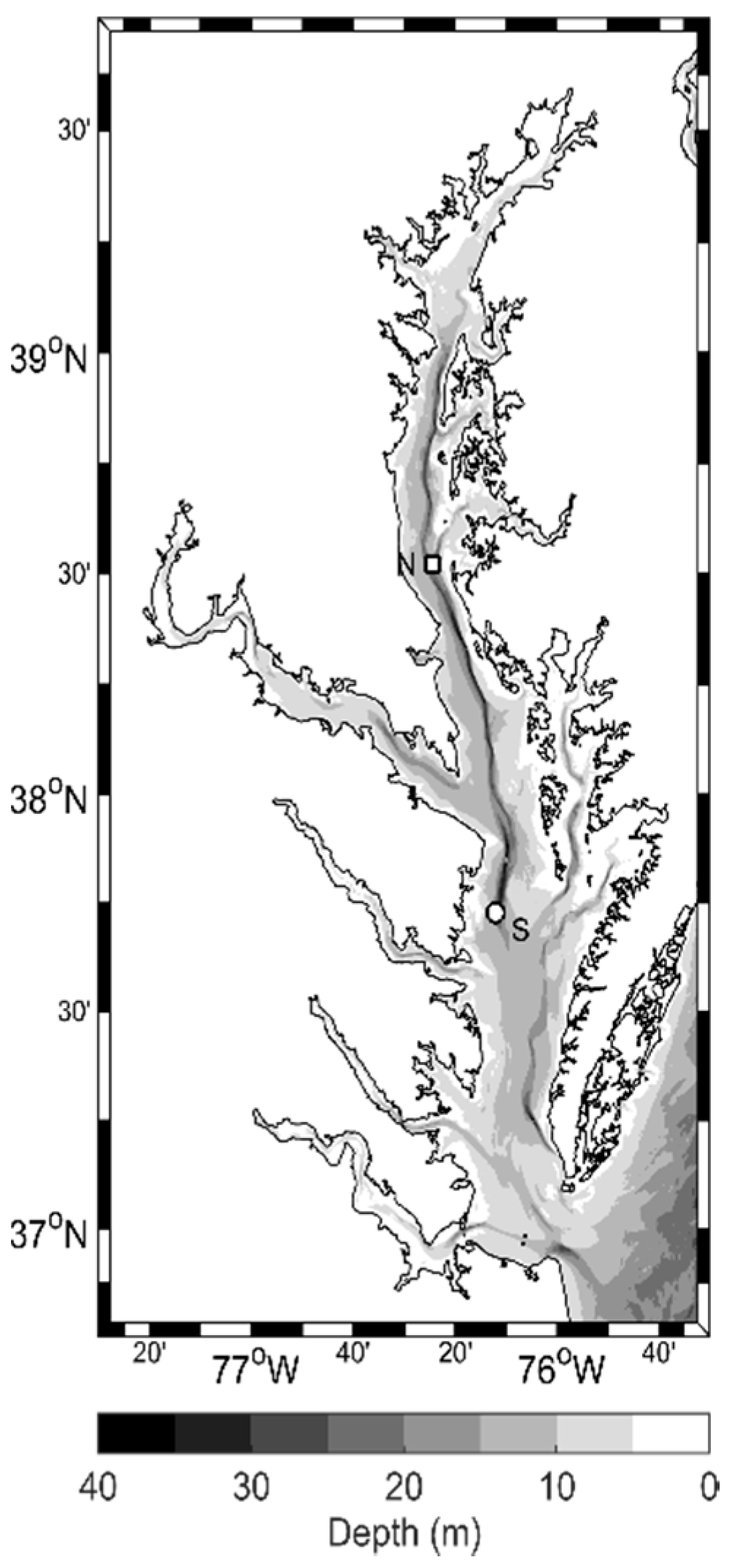
2.1. Cruises and Environmental Data

Six week-long cruises were conducted on the R/V Hugh R. Sharp in the mainstem of the Chesapeake Bay from late spring to autumn (May, July/August, and September) in 2010 and 2011. The vessel anchored at two stations which are approximately 90 km apart, designated North (38°31.32′ N, 076°24.48′ W, depth 28 m) and South (37°43.68′ N, 076°12.0′ W, depth 35 m) (Figure 1). These two stations were selected because both stations were at the mainstem of Chesapeake Bay with comparatively deeper water columns that allow persistent stratification to form, and the North was expected to experience more severe oxygen deficiency over a longer duration compared with the South.

Both biological and hydrographic data were collected. Approximately 2.5 days were spent at each station, with ~27 h at anchor and ~33 h underway near the station conducting net collections for zooplankton and fish. While at anchor, a total of 229 and 223 hourly CTD casts (see the Supplementary Materials) were conducted during the six cruises (

Table A1. The numbers of CTD casts deployed during each cruise.

Cruise	2010	2011
Season
Spring	77	88
Summer	88	69
Autumn	64	66
Total Casts	229	223
		452

) to obtain temperature, salinity, and dissolved oxygen at 0.5-m depth intervals. Cruise details, gear and instrument deployments, and measurements were submitted to the Biological and Chemical Oceanography Data Management Office (BCO-DMO) [64].

2.2. Evaluation of Environmental Oxygen Supplies and Copepod’s Physiological Oxygen Needs

The temperature-specific oxygen demands for the A. tonsa copepod were estimated at each half-meter CTD measurement. First, Q₁₀ of A. tonsa was calculated with respect to salinity (Equation (1), [65]), and oxygen solubility (O₂Sat, [66]) was calculated using the “sw_satO2.m” in the SeaWater MATLAB toolbox [67]. From oxygen solubility, the percentage of oxygen saturation (O₂P_ct, Equation (2)) and saturation partial pressure of environmental oxygen (pO₂, Equation (3)) were calculated. From Q₁₀ and temperature, the temperature-specific critical oxygen partial pressure (P_crit, Equation (4)) and the lethal oxygen partial pressure (P_leth, Equation (5)) could be estimated [12,64,65]. By comparing pO₂ with P_crit and P_leth, the differences between A. tonsa oxygen supply and oxygen demand based on ambient temperature and salinity could be estimated. If pO₂ > P_crit, the metabolism of the copepod A. tonsa is independent of the surrounding pO₂. If pO₂ < P_crit (biological hypoxia), A. tonsa’s metabolism decreases, which may cause copepods to suffer from sublethal effects. If pO₂ < P_leth, the concentration of dissolved oxygen is insufficient to support copepod respiration, causing hypoxia-induced mortality to increase.

$${\mathrm{Q}}_{10}=0.053\times \mathrm{Salinity}+0.705$$

(1)

$${\mathrm{O}}_2\mathrm{Pct}(\%)=\frac{\mathrm{DO}}{{\mathrm{O}}_2\mathrm{Sat}}$$

(2)

$$p{\mathrm{O}}_2=\left(159.27\times {\mathrm{O}}_2\mathrm{Pct}-0.014\right)\times 133.322/1000$$

(3)

$$P_{crit}=7.49{\mathrm{Q}}_{10}{}^{0.1\left(\mathrm{T}-18\right)}+0.59$$

(4)

$$P_{leth}=2.61{\mathrm{Q}}_{10}{}^{0.1\left(\mathrm{T}-18\right)}+0.59$$

(5)

2.3. Estimation of Zooplankton and Planktivorous Fish Concentrations

To document seasonal changes in populations of crustacean zooplankton, gelatinous zooplankton and ichthyoplankton in the mainstem Chesapeake Bay, net collections were conducted at the two stations (North and South) during each cruise; the resulting copepod, gelatinous zooplankton and anchovy datasets were uploaded to the Biological and Chemical Oceanography Data Management Office (BCO-DMO) [68,69,70]. CTD casts were conducted before each series of net tows to determine pycnocline depth and DO levels that guided the selection of net-sampling depths (described in [64]). Each net-collection series included tows with a MOCNESS (Multiple Opening/Closing Net and Environmental Sensing System), a Tucker Trawl, and a mid-water trawl (Table A1 and

Table A2. The numbers of MOCNESS net tows, Tucker Trawls, and mid-water trawls conducted during each cruise.

Cruise	MOCNESS	Tucker Trawls	Mid-Water Trawls
2010
Spring	11	18	0
Summer	11	11	11
Autumn	6	6	6
2011
Spring	8	12	0
Summer	12	12	12
Autumn	12	12	12
Total	60	71	41

). Copepod concentration data were obtained primarily from the MOCNESS tows. However, copepod concentrations in May-2010 (South) were estimated from the Tucker Trawl tows and Sep-2010 (North) from Z-trap deployments (described in [71]) because of MOCNESS mechanical problems. Larval bay anchovies were collected by both the MOCNESS and Tucker Trawl, whereas juvenile and adult bay anchovies were sampled by the mid-water Trawl. Gelatinous zooplankton, primarily bay nettles and ctenophores, were collected by Tucker Trawl. Our study focused on the whole water column; thus, abundances of copepods, jellyfish, ctenophores, and fish were expressed in concentrations (ind. m⁻³) estimated for the entire water depth sampled by each tow.

The MOCNESS [72] had a 0.25 m² mouth and was fitted with six 150-µm mesh nets, and with sensors to measure pressure, temperature, salinity, dissolved oxygen, chlorophyll a fluorescence, flow, turbidity, and photosynthetically active radiation (PAR) in real-time. The MOCNESS was deployed to collect copepods from three layers (above, within, and below pycnocline) and to collect larval bay anchovy from two layers (above and below pycnocline). After each tow, the nets were rinsed, and most adult gelatinous zooplankton were removed by pouring the sample through a 5-mm mesh sieve. The remainder of each sample was concentrated with a 200-µm mesh sieve, preserved in a 4% formaldehyde and seawater solution, and later enumerated in the laboratory. The MOCNESS was inoperative at the South Station during the 2010-May cruise and the 2011-May cruise, and the Tucker Trawl was deployed instead.

The 1-m² Tucker Trawl was fitted with two opening and closing 280 µm-mesh nets and a flowmeter for each net to collect gelatinous zooplankton. During each deployment, each net was opened for two minutes to determine gelatinous zooplankton concentrations from three to four water depth intervals, depending on hydrographic conditions. The nets were rinsed after each trawl and gelatinous zooplankton were separated. If there were more than 30 gelatinous zooplankton of each species, the total numbers of each species were estimated by measuring the wet biovolume of the first 30 randomly selected gelatinous zooplankton and then the total biovolume of all gelatinous zooplankton.

The mid-water trawl, with 18-m² mouth opening and 4-mm cod-end mesh, was deployed twice during each sampling-station occupation. An above- and below-pycnocline trawl deployments collected juvenile and adult bay anchovy at each of the sampling stations during summer and fall cruises. Each deployment was of 20-min duration; the trawl was fished obliquely in two-minute steps within each sampling depth. The effective volume sampled in a 20-min tow was 989 m³ [51]. The number of fish in each trawl sample and relative concentrations (individuals per 20 min) were recorded. Total lengths were measured from a sample of 30 bay anchovies, or all individuals were measured if fewer than 30 were collected from each trawl tow. A representative sample of juvenile and adult bay anchovy was preserved in ethanol for subsequent stomach analysis in the laboratory.

2.4. Nonpredatory Mortality Rates

Neutral red uptake experiments were conducted to estimate the proportion of living and dead copepods in each layer and to calculate the non-predatory mortality rates of copepods [42,73]. Copepods were collected with a CTD rosette by combining water from three 10-L Niskin bottles in each of three discrete layers: surface layer, base of the oxycline, and near the bottom. 90-L were collected: in total, 30 L from each layer. Sampling was repeated three times at each station during all cruises except the spring cruise in 2010. Copepod non-predatory mortality rates (M_np, Equation (6)) were estimated from the percentage of copepod carcasses present in the sample divided by the estimated in situ carcass decomposition time ($\tau )$, a function of copepod dry weight and water temperature (Equation (7), [73,74])

$${\mathrm{M}}_{\mathrm{np}}({\%\mathrm{d}}^{-1})=\frac{\%\mathrm{dead}\mathrm{from}\mathrm{neutral}\mathrm{red}\mathrm{dye}}{\mathrm{carcass}\mathrm{turn}\mathrm{over}\mathrm{time}\left(\tau \right)}$$

(6)

$$\tau =\frac{{\mathrm{Dry}\mathrm{Weight}}_{\mathrm{t}}-{\mathrm{Dry}\mathrm{Weight}}_{\mathrm{i}}}{-4.116\times \left(1-{\mathrm{e}}^{-0.008\mathrm{Temp}}\right)}-1.39$$

(7)

2.5. Statistical Analysis

Principal component analysis (PCA) was applied to assign data from cruises and stations into groups representing comparatively similar environmental conditions. Temperature, salinity, and dissolved oxygen from above, at, and below the pycnocline, selected as the depth of the maximum density gradient for each hourly CTD cast were analyzed in R [75] (

Table 1. Eigenvalue of the principal component analysis of temperature, salinity, and dissolved oxygen (DO) of water sampled by CTD from above, at, and below pycnocline at both the North and South Stations.

	Eigenvalue	Difference	Proportion	Cumulative
1	5.01	2.68	0.56	0.56
2	2.33	1.68	0.26	0.82
3	0.66	0.16	0.07	0.89
4	0.50	0.21	0.06	0.95
5	0.30	0.21	0.03	0.98
6	0.08	0.04	0.01	0.99
7	0.05	0.01	0.01	0.99
8	0.04	0.02	0.00	1.00
9	-	0.02	0.00	1.00

and

Table 2. Eigenvectors of the principal component analysis of temperature, salinity, and dissolved oxygen (DO) of water sampled by CTD from above, at, and below pycnocline at both the North and South Stations.

	Principal Component 1	Principal Component 2
DO above pycnocline	0.35	0.20
DO at pycnocline	0.27	0.33
DO below pycnocline	0.14	0.51
Temp. above pycnocline	−0.38	−0.26
Temp. at pycnocline	−0.39	−0.12
Temp. below pycnocline	−0.42	−0.06
Salinity above pycnocline	−0.33	0.41
Salinity at pycnocline	−0.33	0.39
Salinity below pycnocline	−0.30	0.45

). Based on the PCA results, cruises and stations were first grouped into three temperature groups, designated as cool (C), temperate (T), and warm (W), according to their PC1 scores for which the major loading was temperature. Then, each temperature group was divided into two subgroups, termed less-oxygenated (LO) and more-oxygenated (MO), according to their PC2 scores for which the biggest loading was bottom dissolved oxygen (

Table 3. Grouping cruises (Year-Season (Station)) according to the PCA grouping results. All cruises were designated for three temperature groups according to their PC1 scores (C = Cool, T = Temperate, W = Warm), and each group was divided into two subgroups according to their PC2 scores (LO = Less-oxygenated, MO = More-oxygenated). Bold text indicates the averaged bottom DO < 2 mg L⁻¹, italic text indicates bottom pO₂ < P_crit, and underlined text indicates pO₂ < P_leth.

	LO	MO
C	2011-Spring (N)	2010-Spring (N, S), 2011-Spring (S)
T	2011-Autumn (N)	2011-Autumn (S)
W	2011-Summer (N, S), 2010-Summer (N)	2010-Autumn (N, S), 2010-Summer (S)

). These groups were then used to compare the zooplankton, fish, and gelatinous zooplankton concentrations, as well as the nonpredatory mortality rates.

Differences in the concentrations of copepods, larval and juvenile anchovies, ctenophores, and bay nettles were compared between the LO and MO subgroups within each temperature group (C, T, W) with Kruskal-Wallis test [76] performed in R to test the null hypothesis of no differences among zooplankton concentrations in different oxygenated conditions. Likewise, copepod nonpredatory mortality rates were also compared between hypoxia subgroups within each temperature group to test the null hypothesis of no differences in copepod nonpredatory mortalities under different hypoxic conditions. Note that within the biological hypoxia matrix (pO₂ < P_crit [65], the comparisons between the hypoxia subgroups in the C and T groups were made between normoxic (pO₂ > P_crit) and hypoxic conditions (pO₂ < P_crit), but the comparisons in the W group were made between moderately (pO₂ < P_crit) and severely hypoxic (pO₂ < P_crit) conditions.

To assess the effect of different nets on the capture of larval anchovies, we conducted a permutation t-test, using a 10,000-time rearrangement simulation, using larval anchovy length data from 10 MOCNESS samples and 20 Tucker trawl samples collected at the North station in May 2010.

3. Results

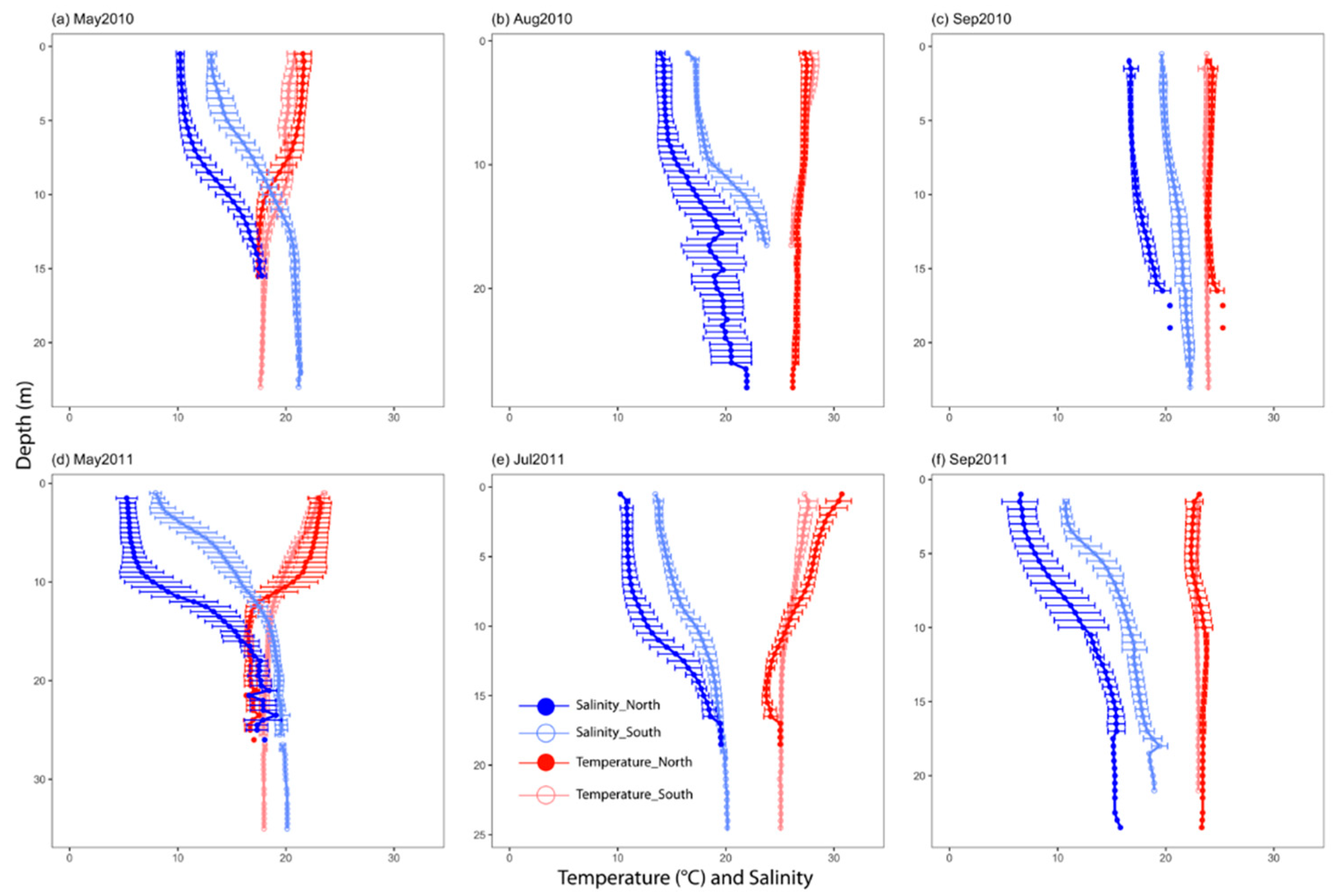
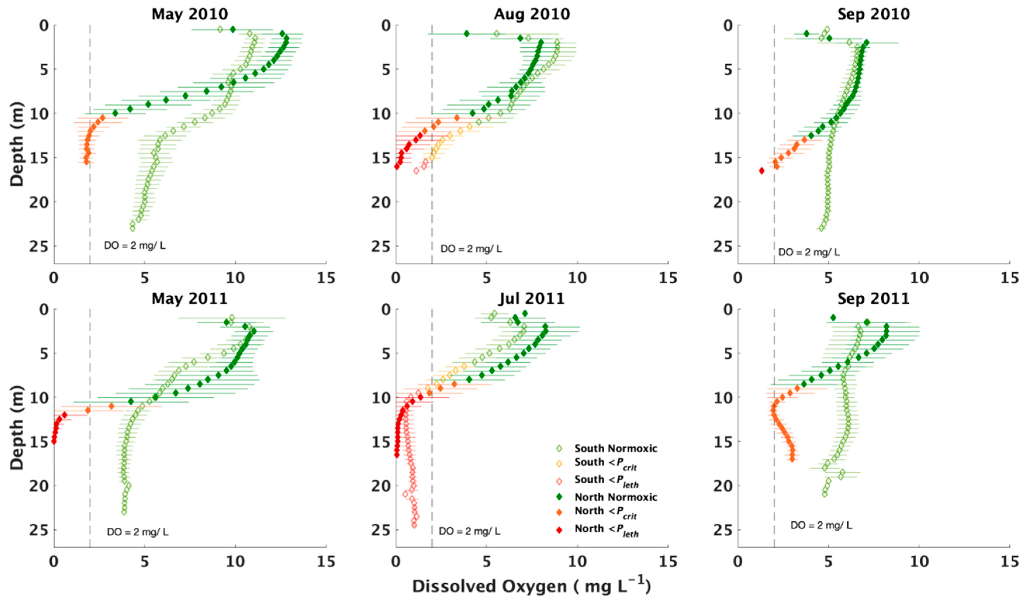
3.1. General Environmental Conditions

Water temperature varied with seasons and years: summer was warmer than spring and fall, and 2011 was warmer than 2010 (Figure 2). The recorded water temperature ranged from 15.5 °C to 34.5 °C, with the highest water temperature observed at the surface of North Station during the 2011-Summer cruise, and the lowest was observed near the bottom of North Station during the 2011-Spring cruise. Salinity primarily varied by depth, station and year: the North Station was less saline than the South Station, especially at the surface, and 2011 was less saline than 2010 (Figure 2). Salinity ranged from 4 to 25, with the highest salinity found near the bottom of the South Station during the 2010-Autumn cruise, and the lowest salinity found at the surface of the North Station during the 2011-Spring cruise.

Dissolved oxygen also varied with depths, stations, seasons, and years. In general, dissolved oxygen was: (1) lower at the North Station than at the South Station; (2) was lower during summer than the other seasons, and (3) was lower in 2011 than in 2010 (Figure 3). Dissolved oxygen ranged from below detectable limits to 15.5 mg L⁻¹; the highest dissolved oxygen was recorded at the surface of the North Station during the 2011-Autumn cruise and the lowest during the 2010-Summer and 2011-Spring and 2011-Summer cruises (Figure 3).

Our two hypoxia indicators (DO and pO₂) mapped different “dead zones” in the Bay, and the volume and duration of the dead zone were more extensive with the biological (pO₂) standard. If only DO concentration was considered as an indicator, oxygen-deficient water in the Chesapeake Bay was mostly confined to the bottom water (Figure 3). However, if the temperature-dependent oxygen demands of the copepod A. tonsa are considered, oxygen-deficient water in the Chesapeake Bay occurred above the pycnocline, and sometimes even near the surface (Figure 3). For example, during the 2011 summer cruise at the South Station, two-thirds of the water column was categorized as biologically hypoxic, and thus, A. tonsa that occurred below 5-m would be stressed by oxygen deficiency. Using the DO indicator, hypoxia was only prevalent in summer, however, if oxygen demand and supply are considered (i.e., pO₂), hypoxic conditions extended into autumn in both years (Figure 3).

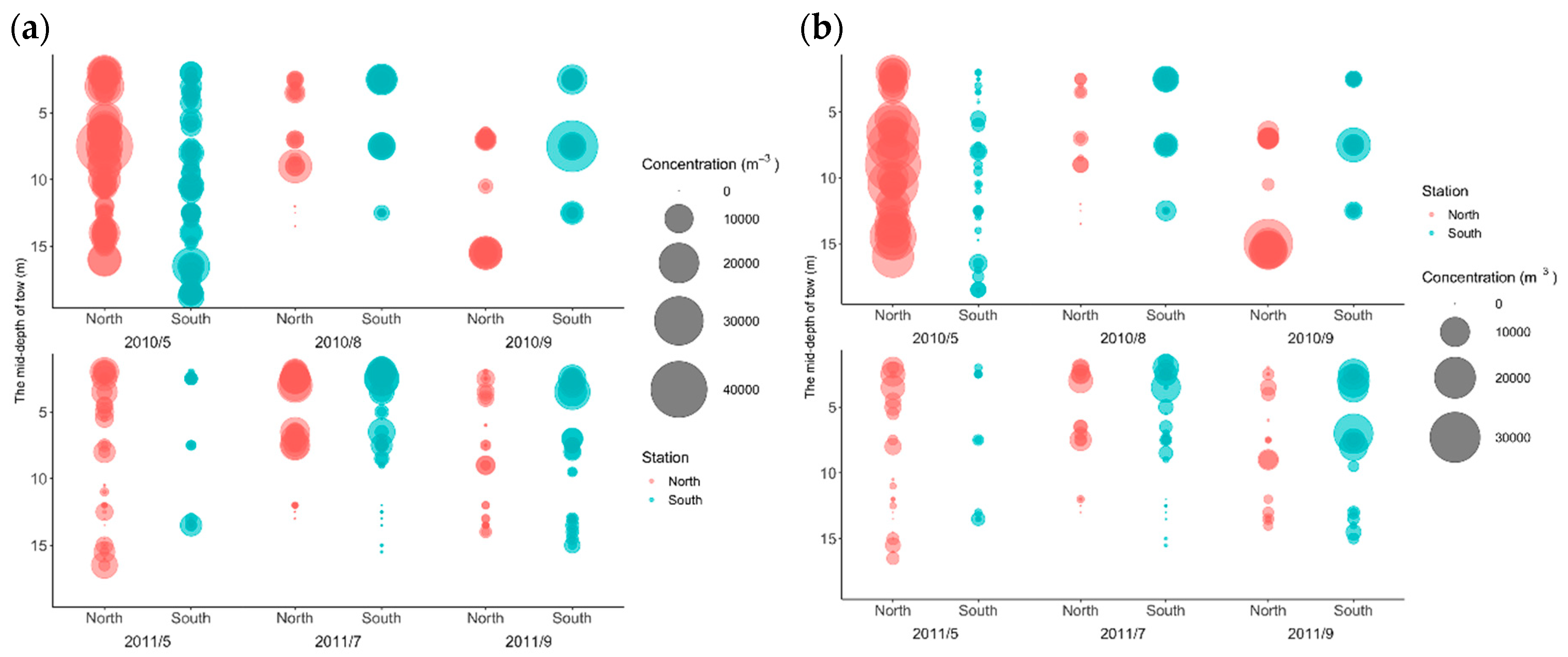
3.2. Zooplankton and Fish Concentrations

In general, there were more copepods and larval bay anchovies observed in spring, more gelatinous zooplankton in summer, and more juvenile bay anchovy in autumn. Overall, there were more crustacean zooplankton and fish in 2010 and more gelatinous zooplankton in 2011 (Figure 4, Figure 5 and Figure 6).

The MOCNESS survey documented the temporal succession of adult A. tonsa, which varied with the development of hypoxia (Figure 4a) In 2010, when hypoxia was more pronounced in summer, the concentrations of adult copepods declined by more than 75% at the North Station and by 20% at the South Station and then began to recover in autumn at both stations (Figure 4a). The oxygen deficiency was worse in 2011 when hypoxic water was observed at the North Station beginning in spring. In addition, Hurricane Irene and Tropical Storm Lee passed Chesapeake Bay approximately one month and two weeks, respectively, before the 2011 autumn cruise. As a result, A. tonsa’s concentrations were low in spring, slightly increased in summer, and declined again in autumn (Figure 4a, lower panel). The temporal changes of A. tonsa copepodites resembled the pattern of adults (Figure 4b). In 2010, the concentrations of copepodites were high at the North Station in spring, lower in summer, and increased in September, while in 2011, the copepodite concentrations remained low in spring and summer and then increased at the South Station in autumn (Figure 4b).

A. mitchilli larvae were most abundant in spring 2010. Juveniles were most abundant in summer 2010 and autumn 2011 (Figure 5). In 2010, the highest concentrations of larval A. mitchilli were observed in May, and abundance declined in summer and remained low in autumn. A similar seasonal pattern was observed in 2011, but concentrations were much lower (Figure 5a). In 2010, the highest concentrations of juvenile A. mitchilli occurred in summer; in 2011, the highest concentrations occurred in autumn (Figure 5b). The permutation t-test to determine whether the Tucker Trawl or MOCNESS net caught larval anchovies of different sizes resulted in a p-value of 0.676, indicating that the larval anchovy’s length distribution (as collected by these two nets) are not significantly different.

Unlike the temporal changes of crustacean zooplankton and planktivorous fish, gelatinous zooplankton peaked during summer, and they were more abundant at the South Station than at the North Station in both years (Figure 6). The highest concentrations of both M. leidyi and C. chesapeakei were observed at the South Station in the summer of 2011. No gelatinous zooplankton were collected in spring, and only a few were found in autumn. In any single Tucker-trawl tow during the six cruises, M. leidyi was at least 50 times more abundant than C. chesapeakei.

3.3. Grouping with PCA Results

Among the nine principal components in our analysis, PC1 explained 56% of the variance, and PC2 explained 26% of the variance; together, these two principal components explained 82% of the variability in environmental conditions (Table 1). Because only PC1 and PC2 had eigenvalues larger than 1, and the cumulative sum increased slowly after PC2, only PC1 and PC2 were retained for further analysis (Table 1). The top three loadings of PC1 were water temperatures in the bottom layer, pycnocline, surface layer, indicating water temperature was the major driving factor of PC1 (Table 2). The top three loadings of PC2 included dissolved oxygen of the bottom layer as well as the salinity of the bottom and surface (Table 2), indicating that bottom dissolved oxygen and salinity in both the bottom and surface layers were the major drivers of PC2 (Table 2). The scatter plot of PC1 and PC2 scores for 335 CTD casts is provided (Figure 7). Because the major loading in PC1 was water temperature, which was negatively related to PC1 (Table 2). All data were grouped into three temperature categories approximately corresponding to PC1 scores −4 to −2, −2 to 0, and 0 to 2, named “Warm (W)”, “Temperate (T)”, and “Cool (C)”, respectively. Because bottom dissolved oxygen was the highest loading on PC2 and dissolved oxygen was positively related to PC2 (Table 2). Each temperature group was further divided into two oxygen subgroups approximately at PC2 = 0, labeled “Less-Oxygenated (LO)”, and “More-Oxygenated (MO)”, respectively, from bottom to top on PC2. The cruises and stations and their corresponding groups are listed in Table 3.

Re-examining the environmental conditions with PCA grouping, the temperature variations among C, T, W group were bigger than the changes among vertical water layers and between LO and MO (Figure 8a). The mean water temperatures were approximately 20 °C, 23 °C, and 26 °C in the C, T, and W groups, respectively. In general, the W group also had higher salinity than the other groups, and the MO subgroups also had higher salinity than the LO subgroup especially in the surface layer (Figure 8b). In each temperature group, the mean dissolved oxygen concentration was higher in the MO subgroup than in the LO subgroup (approximately 7 mg L⁻¹ vs. 5 mg L⁻¹, respectively, Figure 8a,c). Mean dissolved oxygen concentrations were lower in the W group than in the C group, approximately 4.6 mg L⁻¹ in W vs 7.0 mg L⁻¹ in C (Figure 8c). By calculating the gap between oxygen demand at the given temperature and salinity (P_crit) and oxygen supply (pO₂) in the bottom of the water column, the largest oxygen deficiency was observed in C-LO, W-LO, T-LO, in order of severity. (see

Table 4. The Kruskal-Wallis test on differences in concentrations of zooplankton and fish between the more-oxygenated (MO) and less-oxygenated (LO) subgroups within the cool (C), temp (T), and warm (W) groups.

Zooplankton and Fish Concentration
Species	Stage	Group	Sample Size	d.f.	Chi-Square	p-Value
Acartia tonsa	adult	C	103	1	15.1180	0.0001
		T	36	1	9.8108	0.0017
		W	127	1	1.6625	0.1973
Acartia tonsa	copepodite	C	107	1	8.5712	0.0034
		T	36	1	8.8460	0.0029
		W	127	1	25.785	<0.0001
Anchoa mitchilli	larval	C	60	1	6.5997	0.0102
		T	24	1	8.5792	0.0034
		W	58	1	0.5652	0.4522
	juvenile	C *	-	-	-	-
		T	24	1	0.1883	0.6643
		W	58	1	4.3211	0.0376
Mnemiopsis leidyi	adult	C	119	1	2.6121	0.1061
		T	48	1	35.225	<0.0001
		W	116	1	17.545	<0.0001
Chrysaora chesapeakei	medusa	C	0	-	-	-
		T	48	1	1	0.3171
		W	116	1	2.0241	0.1548

* Mid-water trawls were not conducted during the spring cruises, and thus, juvenile A. mitchilli were not sampled in the Cool group.

for details regarding temperature, salinity, and dissolved oxygen concentrations of each layer and group).

All spring cruises were characterized as cool (“C”), and most of the data from spring cruises belong to C-MO except 2011-Spring-North, where the bottom of the water column was severely hypoxic (DO close to 0 mg L⁻¹ and pO₂ < P_leth, Figure 3, Table 3). All summer cruises and the 2010-Autumn cruise fell in the W group. All data from 2010-Autumn and 2010-Summer-South were grouped into W-MO, while data from 2011-Summer and 2010-Summer-North were grouped into W-LO. Only the data from the 2011-Autumn cruise belonged to the T group, and the North Station was characterized as “T-LO”, whereas data collected at the South Station fell into the T-MO group. According to the biological hypoxia matrix (pO₂ < P_crit) [65] and the PCA results, the comparisons between the oxygen deficiency subgroups in the C and T groups were made between normoxic (pO₂ > P_crit) and moderate hypoxic (pO₂ < P_crit), while the comparisons between the oxygen subgroups in the W group were made between moderate and severe hypoxia (pO₂ < P_leth) conditions.

3.4. Effects of Hypoxia

Overall, the less-oxygenated subgroups (LO) had fewer crustacean zooplankton, fewer planktivorous fish, but more gelatinous zooplankton than the more-oxygenated (MO) subgroups (Figure 9, Figure 10 and Figure 11). In all temperature groups, A. tonsa concentrations were lower in the LO than in the MO subgroups; the lowest concentration was found in the T-LO group and highest occurred in the C-MO group (Figure 9). In both the C and the T groups, adult A. tonsa concentrations in the LO groups were only one-third of the copepod concentrations of the MO groups (both p < 0.05, Table 4). In the warm group, the bottom water column was hypoxic in both oxygen subgroups but differed in severity (pO₂ < P_crit in W-MO and pO₂ < P_leth in W-LO, Table 4), and mean A. tonsa concentrations did not differ significantly in the W-LO and W-MO subgroups (Table 4). Similarly, A. tonsa copepodite concentrations were always at least 50% lower in the LO subgroups than in the MO subgroups in all temperature groups (Figure 9b), and the differences between the two oxygenated subgroups were significant in all temperature groups (Table 4).

The concentrations of larval A. mitchilli were also lower in LO subgroups in each temperature group (Figure 5a). Mean larval A. mitchilli concentrations were highest in the C-MO group and lowest in the C-LO and T-LO group (Figure 5a). The differences in larval concentrations among the oxygenated subgroups were significant in the C and T groups (p = 0.0102 and p = 0.0034, respectively), but not in the W group (p = 0.4522, Table 4). The mean densities of juvenile A. mitchilli were highest in the T-MO group and lowest in the W-LO group (Figure 10b). Although there were more juvenile A. mitchilli in the MO subgroup, only the concentrations in the warm group showed a significant difference (p = 0.0376, Table 4).

Unlike the concentrations of copepods and anchovies, there were more gelatinous zooplankton in the LO subgroups (Figure 11). The highest M. leidyi and C. chesapeakei concentrations were found in the W-LO group, while the lowest concentrations were observed in the C-LO group (only M. leidyi and no C. chesapeakei). The LO groups had significantly more M. leidyi associated with the W and T groups (both p < 0.0001, Table 4). The patterns were similar for C. chesapeakei, although the differences between oxygenated subgroups were not significant (Table 4). The difference in concentration between M. leidyi and C. chesapeakei for the oxygenated subgroups increased with temperature (Figure 11), with the biggest difference found in the W-MO group, in which the concentration of M. leidyi was 968 times that of C. chesapeakei.

Copepod non-predatory mortalities were higher under less-oxygenated conditions than under more-oxygenated conditions (Figure 12). The highest daily non-predatory mortality was found in T -LO and lowest in W-MO (50% and 2%, respectively). When compared within the same temperature group, nonpredatory mortality in each LO group was at least twice that of the nonpredatory mortality in the MO group, but only the difference in the warm group was significant (p = 0.008,

Table 5. The Kruskal-Wallis test on differences in Acartia tonsa’s non-predatory mortality between the more-oxygenated and less-oxygenated subgroups within the cool, temperate, and warm groups.

A. tonsa’s Non-Predatory Mortalities
Group	Sample Size	d.f.	Chi-Square	p-Value
Cool	5	1	0.3333	0.5637
Temperate	6	1	2.3333	0.1266
Warm	18	1	6.9286	0.008

).

4. Discussion

4.1. Hydrographical and Biological Hypoxia

In our analysis, the low-dissolved oxygen “dead zone” in the mid-Chesapeake Bay was considerably larger, and the hypoxia event duration lasted longer, if a biological standard (pO₂ < P_crit) was used instead of the commonly-adopted hydrographical hypoxia standard (DO < 2 mg L⁻¹). If we solely applied the hydrographical threshold in our study, the low oxygen regions would be primarily be confined to summertime conditions below the pycnocline. By contrast, using the biological hypoxia threshold, the zone of low oxygen that we surveyed was larger, especially in summer and, at times, was also expressed above the pycnocline (Figure 3). For example, during the 2011 summer cruise at the South Station, two-thirds of the water column was categorized as biologically hypoxic, and more than half of the vertical water column had DO below lethal levels for A. tonsa (pO₂ < P_leth), indicating a highly stressful and even harmful environment to copepods throughout most the water column (Figure 3). Therefore, in 2011 summer at the South Station, A. tonsa lived below 5 m would be affected by oxygen deficiency even when the DO was above 2 mg L⁻¹. In 2011, the hypoxia threshold (P_crit) at the South Station was approximately 4 mg L⁻¹ and not 2 mg L⁻¹ if considering A. tonsa’s metabolic needs and the ambient temperature and salinity.

Although DO < 2 mg L⁻¹ is a commonly-adopted standard for studies of hypoxia effects in estuaries [77], this hydrographical standard does not consider that oxygen solubility varies with temperature and salinity [78] and that diverse species have different oxygen deficiency tolerances [79]. Since oxygen solubility decreases as temperature and salinity increase, using DO < 2 mg L⁻¹ as a definition of hypoxia likely underestimates the severity of oxygen deficiency in warm and saline ecosystems [12]. Compared with other seasonally hypoxic ecosystems, such as the Gulf of Mexico, temperature and salinity in the Chesapeake Bay are moderate. However, Chesapeake Bay can be warm and saline during summer in its down-estuary region, where hypoxia is often considered less severe compared to more the up-estuary portions of the Bay. For example, during the 2011 summer cruise, DO concentrations at the South station were similar to those measured at the same depth at the North station. But by contrast, a much higher percentage of the water column was biologically hypoxic at the South station due to high salinity in the deeper water column of the South station ([64]). Under these conditions, the water column of the South station provided a less suitable habitat for A. tonsa than that of the North station, even though the DO concentration at the North station was similar or higher. Consequently, habitat degradation due to hypoxia in the lower Chesapeake Bay may be underestimated if the fixed hydrographical standard (i.e., 2 mg L⁻¹) for defining hypoxia is used.

In addition to oxygen supply varying with temperature and salinity, oxygen demands also vary among species and life stages. Typically, fast-swimming species and younger individuals require more oxygen at the same temperature and salinity than do drifting species and older individuals [43]. In this study, we compared the oxygen supply and demand of adult A. tonsa and concluded that the area and duration of biological hypoxia (pO₂ < P_crit) was larger and longer than hydrographical hypoxia (DO < 2 mg L⁻¹). In contrast, gelatinous zooplankton are known to be more tolerant of hypoxia [57] than copepods. For example Decker et al. (2004) observed A. tonsa’s jumping frequency decreased with decreasing dissolved oxygen, while the clearance rate of the gelatinous planktivore M. leidyi was little affected by low dissolved oxygen concentrations. The P_crit of M. leidyi, an important gelatinous predator in the mainstem Chesapeake Bay during summer, is 7 kPa at 25 °C [57,80], which is about half the P_crit of A. tonsa at the same temperature (13 kPa, [65]. Accordingly, the biologically defined hypoxic regions for M. leidyi would be smaller than the hydrographically-defined zone of hypoxia in the Bay. Applying this same reasoning, areas where biologically hypoxic conditions occur for large and fast swimming species, like striped bass, would be larger than the hydrographically determined zone of hypoxia in the Bay. Considering that responses of organisms to low-dissolved oxygen are not universal, we recommend that future studies of hypoxia impacts on ecosystems should not only focus on dissolved oxygen concentrations but should also consider the species-specific effects of temperature and salinity and biologically-relevant hypoxic conditions.

4.2. Seasonal and Episodic Hypoxia

Species respond differently to hypoxia at various temporal scales. In a permanently hypoxic ecosystem, e.g., in the ocean’s oxygen minimum zone, many organisms evolve physiological adaptations and genetic modifications to cope with a low-dissolved oxygen environment through enhancing oxygen absorption (i.e., increasing hemoglobin O₂ affinity and gill surface area) and decreasing oxygen demands (i.e., reducing red blood cell ATP concentration) [81,82,83,84]. Many species in the oxygen minimum zone, particularly krill and myctophid fishes, use hypoxic conditions to their advantage and take refuge from visually predators during daytime [85]. On the other hand, organisms living in non-permanent hypoxic conditions tend to rely on behavioral adaptations or metabolic suppression to cope with temporary adverse conditions [86]. Thus, oxygen deficiency acts as a stressor rather than a refuge for organisms living in episodic or seasonally hypoxic ecosystems, often characterized as coastal dead zones.

Hypoxia in the Chesapeake Bay is seasonal and especially pronounced in summer. The PCA analysis indicated that in 2010 and 2011, water during summer was distinguished from water in spring as being warmer, more saline, and having less dissolved oxygen in the bottom layers. Although the oxygen deficiency is temporary and localized, many studies have found adverse effects of summer bottom hypoxia on vertical distributions of organisms [59,87,88], abundance [41], and diversity [89]. Previous studies found that copepods show different diel migration patterns under seasonal hypoxia [64] and increased non-predatory mortality in summer [42].

The PCA results also indicated that water during the 2011 autumn cruise, which occurred after Hurricane Irene (27 August 2011) and Tropical Storm Lee (7–10 September 2011) affected the region, could be distinguished from water conditions during our other cruises (Figure 7). The water column was cooler, less saline, and less oxygenated in September 2011 relative to water samples collected in 2010 at the same location and season. Significant weather events like hurricanes and tropical storms could cause a hypoxia event by introducing large amounts of freshwater runoff and organic matter. Palinkas et al. described Hurricane Irene as a wind and sediment-resuspension event, while Tropical Storm Lee was a hydrographical and sediment-deposition event [90]. Tropical Storm Lee brought high streamflow (22,002 m³ s⁻¹) to the Susquehanna River and resulted in the second-highest recorded discharge behind Tropical Storm Agnes in 1972 [91]. As a result, salinities measured during the 2011 autumn cruise were much lower than those measured in the previous year. Other studies in estuaries also have observed short-term hypoxia after hurricanes [92,93], and sometimes the recovery to baseline conditions took months [94]. Similarly, early-fall hypoxia was soon reestablished after Hurricane Isabel impacted the Chesapeake Bay, and the resuspension of nutrients into the upper water column led to a large diatom bloom, followed by a dinoflagellate bloom [95]. The effects of episodic hypoxia resulting from storms are less studied. While unplanned, we may have observed the effects of Hurricane Irene and Tropical Storm Lee on the Chesapeake Bay ecosystem during the 2011 autumn cruise. In this study, both seasonal and episodic hypoxia were observed, but differences found were dictated by snapshots of the two stations during the 3 seasons in 2 years. More research, such as higher frequency sampling before and after weather events and long-term observation at more stations across different geographic conditions, are needed to assess the variability and to understand the differences and similarities of seasonal hypoxia and episodic hypoxia on zooplankton composition and foodweb interactions.

4.3. Strengths and Limitations of the PCA Grouping Method and Our Sampling Regime

Because temperature, salinity, and dissolved oxygen varied differently with depths, stations, season, and years, a PCA method was adopted to help group data, enabling comparison of different hypoxic conditions while temperature and salinity were comparatively similar. By only comparing the oxygenated subgroups within the same temperature group, we could understand the effects of hypoxia on organisms, while isolating effects of temperature. Although we were not able to isolate the effects of salinity, all species examined in this study were euryhaline species and are native to this partially mixed estuary. For example, Chesapeake Bay organisms occur at a wide range of salinities: A. tonsa < 5–38, M. leidyi 3.4–33, C. chesapeakei 10–26, and A. mitchilli 0–45, in the Chesapeake Bay [51,96,97,98,99,100]. The salinity of the sampling region ranged from 8 to 25 (Figure 8), which is within the range of salinity habitat of the species studied. Although A. tonsa’s oxygen demands increase when salinity diverges from its natural habitat and their mortality increases when exposed to salinity changes > 10–15 [96,101,102], the salinity differences between LOs and MOs in our study were small (i.e., 3–5,

Table A5. Mean (±S.D.) temperature, salinity, partial pressure of dissolved oxygen (pO₂) in three water layers (Surf. = above the pycnocline, Pyc. = within the pycnocline, Bot. = below the pycnocline), and the corresponding critical partial oxygen pressure (P_crit) and lethal oxygen partial pressure (P_leth) in each temperature (C = Cool, T = Temperate, and W = Warm) and dissolved oxygen subgroups (LO = less oxygenated, MO = more oxygenated). Sample sizes indicate the total numbers of CTD casts in each group. Bold pO₂ values indicate pO₂ < P_crit (Biological hypoxia), and bold and italic values indicate pO₂ < P_leth.

Group	Sample Size		Layer	Temperature				Salinity				pO2				Pcrit		Pleth
	LO	MO		LO		MO		LO		MO		LO		MO		LO	MO	LO	MO
C	28	87	Surf.	22.69	±0.53	21.19	±1.10	5.86	±0.40	11.56	±2.30	23.48	±2.32	26.79	±2.95	8.13	8.77	3.22	3.44
			Pyc.	19.95	±1.81	20.39	±1.55	8.06	±2.22	13.57	±2.92	13.80	±5.39	21.87	±5.06	8.26	8.74	3.26	3.43
			Bot.	17.18	±0.50	18.51	±0.75	12.76	±1.14	17.44	±1.75	1.48	±1.36	11.79	±4.33	7.88	8.27	3.13	3.27
T	23	26	Surf.	22.64	±0.23	22.94	±0.07	8.22	±1.12	11.22	±1.36	17.39	±3.93	17.14	±3.60	8.55	9.12	3.36	3.56
			Pyc.	23.14	±0.49	22.91	±0.07	11.06	±1.92	14.30	±1.52	16.92	±5.65	17.33	±4.17	9.13	9.62	3.57	3.74
			Bot.	23.61	±0.22	22.90	±0.06	13.61	±0.93	16.42	±0.79	7.36	±1.68	16.37	±1.36	9.73	9.95	3.78	3.85
W	87	86	Surf.	26.12	±1.44	26.27	±1.80	14.35	±2.27	17.50	±2.16	15.34	±2.82	19.18	±2.41	10.81	11.82	4.15	4.50
			Pyc.	24.87	±0.89	25.95	±1.62	15.99	±1.51	19.05	±1.94	11.82	±4.59	15.68	±3.74	10.72	12.09	4.12	4.60
			Bot.	24.39	±0.60	25.69	±1.34	17.85	±0.93	20.85	±1.53	4.06	±4.34	8.34	±5.61	10.91	12.41	4.19	4.71

). By comparison, the differences in bottom dissolved oxygen between LOs and MOs in this study provided either insufficient or sufficient oxygen concentrations to support the basic metabolism of A. tonsa (Table A5). The loading of salinity in the PCA analysis was smaller than the temperature in PC1 and less than bottom dissolved oxygen in PC2, and thus, differences in bottom dissolved oxygen were larger than the differences in salinities between the LO and the MO subgroups. Therefore, we reasoned that the moderate salinity fluctuations observed in the six cruises would have a smaller influence than temperature and bottom dissolved oxygen on zooplankton and planktivorous fish concentrations and copepod non-predatory mortality. More research is needed to clarify the effects of interactions of salinity and dissolved oxygen on organism occurrence and concentration.

The time sensitive nature of research cruise sampling meant that if we missed a sampling opportunity, we may not have been able to do it again. So, when presented with mechanical failures we decided to collect the samples in the best possible way, even if it was not optimal. Thus, different nets were used at certain times in order to not miss a sampling opportunity. Skjodal et al. suggest that net mesh should effectively retain organisms whose smallest dimension is approximately 2/3 of the mesh size [103]. In the case of the Tucker Trawl used here, with 280 µm mesh, we expect it to retain organisms > 187 µm in size. The MOCNESS mesh size was 200 µm. Estimated widths for adult A. tonsa from Chesapeake Bay during May 2010, when the Tucker Trawl was used a substitute for the MOCNESS, was 297 and 279 µm for female and male A. tonsa, respectively (Pierson, unpubl.), and Elliott et al. (2013) estimated a width of 262 µm for adult A. tonsa from the same region [42]. These widths are well above the minimum size for capturing A. tonsa adults and thus suggest no difference in catchability between the MOCNESS and Tucker Trawl, which were both towed in an oblique manner. The Z-trip was used to collect zooplankton samples in a vertical manner, and sampled a lower volume of water, but as it had the same mesh size as the MOCNESS, and we anticipate similar catchability between these nets. Our test of the catchability of larval between the Tucker Trawl and the MOCNESS indicated no differences in the sizes of individuals caught, based on a permutation t-test of 10,000 simulations of the data, which further gives us confidence in our sampling despite the fact that we were compelled to use different nets at certain times.

4.4. Copepod’s Predators in Hypoxia

A. tonsa’s predators responded differently toward hypoxia in our study: more M. leidyi and C. chesapeakei but fewer A. mitchilli under hypoxic conditions. The reasons of fewer larval and juvenile A. mitchilli were observed under hypoxic conditions could be decreasing habitat, reducing growth rates, and increasing mortality at young stages, which could also result in declining species diversity [104,105,106]. An individual-based model developed for Chesapeake Bay indicated that the mortality rate of A. mitchilli larvae would increase, as would spatial overlaps among A. mitchilli and its predators when bottom waters were hypoxic [54,104]. On the contrary, more gelatinous zooplankton were found under hypoxic conditions, and overall larger ctenophore populations than those of C. chesapeakei. Long-term decreases in C. chesapeakei have been observed in the Chesapeake Bay mainstem region, leading to reduced predation impact upon M. leidyi and a corresponding increase in the M. leidyi population in the mainstem region [14,107]. Hypoxia could contribute to the population decline in C. chesapeakei observed in the Chesapeake Bay, because ctenophores are known to be better oxyregulators than medusae [80], and M. leidyi’s life cycle does not have a benthic stage like C. chesapeakei, whose polyp stage has been shown to be vulnerable to hypoxia when held at 0.5 mg L⁻¹ for more than 5 days [108]. Other potential contributing factors to the population shift include decreased availability of benthic habitat (i.e., oyster shell) for C. chesapeaki’s polyps due to declining oyster populations [109,110]. Additionally, the declining oyster population is hypothesized to exacerbate the effects of anthropogenic nutrient enrichment on phytoplankton production [111]. Resulting eutrophication, in addition to favoring increased hypoxia, may favor microzooplankton and filter feeders like M. leidyi [112]. Furthermore, warmer and shorter winters in the long-term could strengthen stratification and increase the severity and duration of summer hypoxia, while also increasing M. leidyi’s over-winter survival rate and contributing to its reproductive capacity in earlier and warmer springs [113,114]. Although M. leidyi has received less attention from the general public relative to the more noticeable, stinging C. chesapeakei, the shift in population sizes of these two gelatinous species is important because M. leidyi is able to prey more heavily on copepods than C. chesapeakei of the same size. Thus, M. leidyi’s impact on the plankton foodweb is expected to increase with its growing population [107,115]. The impact of eutrophication-induced hypoxia on an ecosystem can be systemic, ranging from species to habitat to food web structure. Such an ecosystem is less resilient and is usually dominated by pelagic algae, microbial loops, smaller zooplankton, filter feeders, and smaller fish [7,14,15,116,117,118]. More research is still needed to understand the interaction of hypoxia and predator-prey interaction in the field.

5. Conclusions

Crustacean zooplankton (A. tonsa) and planktivorous fish (larval and juvenile A. mitchilli) concentrations tended to be lower under hypoxia, while gelatinous zooplankton populations (both M. leidyi and C. chesapeakei) increased under the same conditions. These population trends relative to hypoxia were consistent among different temperature conditions and were pronounced relative to the influence of seasonality. Neutral red staining indicated high non-predatory copepod mortality under hypoxic conditions and implied a direct linkage between low dissolved oxygen and reduced copepod abundances. These findings confirm the role of hypoxia as a source of direct mortality for copepods in the Chesapeake Bay, and hypoxia directly associates with more gelatinous zooplankton population and less planktivorous fish in addition to seasonality, implying potential predator–prey dynamic changes in this system.

References

1. Rabalais, N.N.; Diaz, R.J.; Levin, L.A.; Turner, R.E.; Gilbert, D.; Zhang, J. Dynamics and distribution of natural and human-caused hypoxia. Biogeosciences 2010, 7, 585–619. [Google Scholar] [CrossRef] [Green Version]
2. Rhein, M.; Rintoul, S.R.; Aoki, S.; Campos, E.; Chambers, D.; Feely, R.A.; Gulev, S.; Johnson, G.C.; Josey, S.A.; Kostianoy, A.; et al. Observations: Ocean; Cambridge University Press: Cambridge, UK, 2013; pp. 255–315. [Google Scholar]
3. Diaz, R.J.; Rosenberg, R. Spreading dead zones and consequences for marine ecosystems. Science 2008, 321, 926–929. [Google Scholar] [CrossRef] [PubMed]
4. Libes, S. Introduction to Marine Biogeochemistry; Academic Press: Cambridge, MA, USA, 2011; ISBN 0-08-091664-3. [Google Scholar]
5. Cowan, J.L.; Boynton, W.R. Sediment-water oxygen and nutrient exchanges along the longitudinal axis of Chesapeake Bay: Seasonal patterns, controlling factors and ecological significance. Estuaries 1996, 19, 562–580. [Google Scholar] [CrossRef]
6. Hagy, J.D.; Boynton, W.R.; Keefe, C.W.; Wood, K.V. Hypoxia in Chesapeake Bay, 1950–2001: Long-term change in relation to nutrient loading and river flow. Estuaries 2004, 27, 634–658. [Google Scholar] [CrossRef]
7. Kemp, W.M.; Boynton, W.R.; Adolf, J.E.; Boesch, D.F.; Boicourt, W.C.; Brush, G.; Cornwell, J.C.; Fisher, T.R.; Glibert, P.M.; Hagy, J.D.; et al. Eutrophication of Chesapeake Bay: Historical trends and ecological interactions. Mar. Ecol. Prog. Ser. 2005, 303, 1–29. [Google Scholar] [CrossRef]
8. Murphy, R.R.; Kemp, W.M.; Ball, W.P. Long-term trends in Chesapeake Bay seasonal hypoxia, stratification, and nutrient loading. Estuaries Coasts 2011, 34, 1293–1309. [Google Scholar] [CrossRef]
9. Breitburg, D.; Levin, L.A.; Oschlies, A.; Grégoire, M.; Chavez, F.P.; Conley, D.J.; Garçon, V.; Gilbert, D.; Gutiérrez, D.; Isensee, K.; et al. Declining oxygen in the global ocean and coastal waters. Science 2018, 359, eaam7240. [Google Scholar] [CrossRef] [Green Version]
10. Deutsch, C.; Brix, H.; Ito, T.; Frenzel, H.; Thompson, L. Climate-Forced Variability of Ocean Hypoxia. Science 2011, 333, 336–339. [Google Scholar] [CrossRef] [Green Version]
11. Najjar, R.G.; Pyke, C.R.; Adams, M.B.; Breitburg, D.; Hershner, C.; Kemp, M.; Howarth, R.; Mulholland, M.R.; Paolisso, M.; Secor, D.; et al. Potential climate-change impacts on the Chesapeake Bay. Estuar. Coast. Shelf Sci. 2010, 86, 1–20. [Google Scholar] [CrossRef]
12. Roman, M.R.; Brandt, S.B.; Houde, E.D.; Pierson, J.J. Interactive Effects of Hypoxia and Temperature on Coastal Pelagic Zooplankton and Fish. Front. Mar. Sci. 2019, 6, 139. [Google Scholar] [CrossRef] [Green Version]
13. Breitburg, D.L.; Loher, T.; Pacey, C.A.; Gerstein, A. Varying Effects of Low Dissolved Oxygen on Trophic Interactions in an Estuarine Food Web. Ecol. Monogr. 1997, 67, 489–507. [Google Scholar] [CrossRef]
14. Kimmel, D.G.; Boynton, W.R.; Roman, M.R. Long-term decline in the calanoid copepod Acartia tonsa in central Chesapeake Bay, USA: An indirect effect of eutrophication? Estuar. Coast. Shelf Sci. 2012, 101, 76–85. [Google Scholar] [CrossRef]
15. Wu, R.S. Hypoxia: From molecular responses to ecosystem responses. Mar. Pollut. Bull. 2002, 45, 35–45. [Google Scholar] [CrossRef]
16. Noone, K.J.; Diaz, R.J.; Sumaila, U.R. Managing Ocean. Environments in a Changing Climate: Sustainability and Economic Perspectives, 1st ed.; Elsevier: Burlington, MA, USA, 2013; ISBN 978-0-12-407668-6. [Google Scholar]
17. Buchheister, A.; Bonzek, C.F.; Gartland, J.; Latour, R.J. Patterns and drivers of the demersal fish community of Chesapeake Bay. Mar. Ecol. Prog. Ser. 2013, 481, 161–180. [Google Scholar] [CrossRef]
18. Lipton, D.; Hicks, R. The cost of stress: Low dissolved oxygen and economic benefits of recreational striped bass (Morone saxatilis) fishing in the Patuxent River. Estuaries 2003, 26, 310–315. [Google Scholar] [CrossRef]
19. Diaz, R.J.; Rosenberg, R. Marine benthic hypoxia: A review of its ecological effects and the behavioural responses of benthic macrofauna. Oceanogr. Mar. Biol. Annu. Rev. 1995, 33, 245–303. [Google Scholar]
20. Heinle, D.R. Production of a calanoid copepod, Acartia tonsa, in the Patuxent River estuary. Chesap. Sci. 1966, 7, 59–74. [Google Scholar] [CrossRef]
21. Lippson, A.J.; Lippson, R.L. Life in the Chesapeake Bay; JHU Press: Baltimore, MD, USA, 2006; ISBN 0-8018-8337-7. [Google Scholar]
22. Olson, M.M. Ecological Studies in the Middle Reach of Chesapeake Bay; Springer: Berlin/Heidelberg, Germany, 1987; Volume 23. [Google Scholar]
23. Steinberg, D.K.; Condon, R.H. Zooplankton of the York River. J. Coast. Res. 2009, 14, 66–69. [Google Scholar] [CrossRef]
24. Wilson, C.B. The copepod crustaceans of Chesapeake Bay. Proc. U. S. Natl. Mus. 1932, 80, 1–54. [Google Scholar] [CrossRef]
25. Alekseev, V.R.; Souissi, A. A new species within the Eurytemora affinis complex (Copepoda: Calanoida) from the Atlantic Coast of USA, with observations on eight morphologically different European populations. Zootaxa 2011, 2767, 41–56. [Google Scholar] [CrossRef]
26. Kimmel, D.G.; Roman, M.R. Long-term trends in mesozooplankton abundance in Chesapeake Bay, USA: Influence of freshwater input. Mar. Ecol. Prog. Ser. 2004, 267, 71–83. [Google Scholar] [CrossRef]
27. White, J.R.; Roman, M.R. Seasonal study of grazing by metazoan zooplankton in the mesohaline Chesapeake Bay. Mar. Ecol. Prog. Ser. 1992, 86, 251–261. [Google Scholar] [CrossRef]
28. Bayha, K.M.; Collins, A.G.; Gaffney, P.M. Multigene phylogeny of the scyphozoan jellyfish family Pelagiidae reveals that the common U.S. Atlantic sea nettle comprises two distinct species (Chrysaora quinquecirrha and C. chesapeakei). PeerJ 2017, 5, e3863. [Google Scholar] [CrossRef] [PubMed] [Green Version]
29. Burrell, V.G.; Van Engel, W.A. Predation by and distribution of a ctenophore, Mnemiopsis leidyi A. Agassiz, in the York River estuary. Estuar. Coast. Mar. Sci. 1976, 4, 235–242. [Google Scholar] [CrossRef]
30. Calder, D.R. Hydroids and Hydromedusae of Southern Chesapeake Bay; CAB International: Wallingford, UK, 1971. [Google Scholar]
31. Mayer, A.G. Medusae of the World: The Scyphomedusae; Carnegie Institution of Washington: Washington, DC, USA, 1910. [Google Scholar]
32. Mayor, A.G. Ctenophores of the Atlantic Coast of North. America; Carnegie Institution of Washington: Washington, DC, USA, 1912. [Google Scholar]
33. Morales-Alamo, R.; Haven, D.S. Atypical mouth shape of polyps of the jellyfish, Aurelia aurita, from Chesapeake Bay, Delaware Bay, and Gulf of Mexico. Chesap. Sci. 1974, 15, 22–29. [Google Scholar] [CrossRef]
34. Purcell, J.E.; Nemazie, D.A. Quantitative feeding ecology of the hydromedusan Nemopsis bachei in Chesapeake Bay. Mar. Biol. 1992, 113, 305–311. [Google Scholar]
35. Stone, S.L. Distribution and Abundance of Fishes and Invertebrates in Mid-Atlantic Estuaries; US Department of Commerce; National Oceanic and Atmospheric Administration: Silver Spring, MD, USA, 1994.
36. Wang, S.B.; Houde, E.D. Energy storage and dynamics in bay anchovy Anchoa mitchilli. Mar. Biol. 1994, 121, 219–227. [Google Scholar] [CrossRef]
37. Newberger, T.A.; Houde, E.D. Population biology of bay anchovy Anchoa mitchilli in the mid Chesapeake Bay. Mar. Ecol. Prog. Ser. 1995, 116, 25–37. [Google Scholar] [CrossRef]
38. Murdy, E.O.; Birdsong, R.S.; Musick, J.A. Fishes of Chesapeake Bay; Smithsonian Institution Press: Washington, DC, USA, 1997; ISBN 1-56098-638-7. [Google Scholar]
39. Jung, S.; Houde, E.D. Spatial and temporal variabilities of pelagic fish community structure and distribution in Chesapeake Bay, USA. Estuar. Coast. Shelf Sci. 2003, 58, 335–351. [Google Scholar] [CrossRef]
40. Olney, J.E. Eggs and early larvae of the bay anchovy, Anchoa mitchilli, and the weakfish, Cynoscion regalis, in lower Chesapeake Bay with notes on associated ichthyoplankton. Estuaries 1983, 6, 20–35. [Google Scholar] [CrossRef]
41. Roman, M.R.; Gauzens, A.L.; Rhinehart, W.K.; White, J.R. Effects of low oxygen waters on Chesapeake Bay zooplankton. Limnol. Oceanogr. 1993, 38, 1603–1614. [Google Scholar] [CrossRef]
42. Elliott, D.T.; Pierson, J.J.; Roman, M.R. Copepods and hypoxia in Chesapeake Bay: Abundance, vertical position and non-predatory mortality. J. Plankton Res. 2013, 35, 1027–1034. [Google Scholar] [CrossRef] [Green Version]
43. Ekau, W.; Auel, H.; Poertner, H.; Gilbert, D. Impacts of hypoxia on the structure and processes in pelagic communities (zooplankton, macro-invertebrates and fish). Biogeosciences 2010, 7, 1669–1699. [Google Scholar] [CrossRef] [Green Version]
44. Lutz, R.V.; Marcus, N.H.; Chanton, J.P. Effects of low oxygen concentrations on the hatching and viability of eggs of marine calanoid copepods. Mar. Biol. 1992, 114, 241–247. [Google Scholar] [CrossRef]
45. Marcus, N.H.; Richmond, C.; Sedlacek, C.; Miller, G.A.; Oppert, C. Impact of hypoxia on the survival, egg production and population dynamics of Acartia tonsa Dana. J. Exp. Mar. Biol. Ecol. 2004, 301, 111–128. [Google Scholar] [CrossRef]
46. Richmond, C.; Marcus, N.H.; Sedlacek, C.; Miller, G.A.; Oppert, C. Hypoxia and seasonal temperature: Short-term effects and long-term implications for Acartia tonsa Dana. J. Exp. Mar. Biol. Ecol. 2006, 328, 177–196. [Google Scholar] [CrossRef]
47. Vargo, S.L.; Sastry, A.N. Acute temperature and low dissolved oxygen tolerances of brachyuran crab (Cancer irroratus) larvae. Mar. Biol. 1977, 40, 165–171. [Google Scholar] [CrossRef]
48. Chesney, E.J.; Houde, E.D. Laboratory Studies on the Effects of Hypoxic Waters on the Survival of Eggs and Yolk-sac Larvae of the Bay Anchovy, Anchoa mitchilli; Center for Environmental Science, Chesapeake Biological Laboratory: Solomons, MD, USA, 1989; pp. 184–191. [Google Scholar]
49. Houde, E.D.; Zastrow, C.E. Bay anchovy Anchoa mitchilli. In Habitat Requirements for Chesapeake Bay Living Resources; Chesapeake Bay Program Living Resources Subcommittee: Annapolis, MD, USA, 1991; pp. 8-1–8-14. [Google Scholar]
50. MacGregor, J.M.; Houde, E.D. Onshore-offshore pattern and variability in distribution and abundance of bay anchovy Anchoa mitchilli eggs and larvae in Chesapeake Bay. Mar. Ecol. Prog. Ser. 1996, 138, 15–25. [Google Scholar] [CrossRef]
51. Jung, S.; Houde, E.D. Recruitment and spawning-stock biomass distribution of bay anchovy (Anchoa mitchilli) in Chesapeake Bay. Fish. Bull. 2004, 102, 63–77. [Google Scholar]
52. Taylor, J.C.; Rand, P.S.; Jenkins, J. Swimming behavior of juvenile anchovies (Anchoa spp.) in an episodically hypoxic estuary: Implications for individual energetics and trophic dynamics. Mar. Biol. 2007, 152, 939–957. [Google Scholar] [CrossRef]
53. Ludsin, S.A.; Zhang, X.; Brandt, S.B.; Roman, M.R.; Boicourt, W.C.; Mason, D.M.; Costantini, M. Hypoxia-avoidance by planktivorous fish in Chesapeake Bay: Implications for food web interactions and fish recruitment. J. Exp. Mar. Biol. Ecol. 2009, 381, S121–S131. [Google Scholar] [CrossRef]
54. Adamack, A.; Rose, K.; Breitburg, D.; Nice, A.; Lung, W. Simulating the effect of hypoxia on bay anchovy egg and larval mortality using coupled watershed, water quality, and individual-based predation models. Mar. Ecol. Prog. Ser. 2012, 445, 141–160. [Google Scholar] [CrossRef] [Green Version]
55. North, E.W.; Houde, E.D. Distribution and transport of bay anchovy (Anchoa mitchilli) eggs and larvae in Chesapeake Bay. Estuar. Coast. Shelf Sci. 2004, 60, 409–429. [Google Scholar] [CrossRef]
56. Breitburg, D.L. Behavioral response of fish larvae to low dissolved oxygen concentrations in a stratified water column. Mar. Biol. 1994, 120, 615–625. [Google Scholar] [CrossRef]
57. Purcell, J.E.; Breitburg, D.L.; Decker, M.B.; Graham, W.M.; Youngbluth, M.J.; Raskoff, K.A. Pelagic cnidarians and ctenophores in low dissolved oxygen environments: A review. In Coastal Hypoxia: Consequences for Living Resources and Ecosystems; American Geophyical Union: Washington, DC, USA, 2001; pp. 77–100. [Google Scholar]
58. Breitburg, D.L.; Adamack, A.; Rose, K.A.; Kolesar, S.E.; Decker, B.; Purcell, J.E.; Keister, J.E.; Cowan, J.H. The pattern and influence of low dissolved oxygen in the Patuxent River, a seasonally hypoxic estuary. Estuaries 2003, 26, 280–297. [Google Scholar] [CrossRef]
59. Keister, J.E.; Houde, E.D.; Breitburg, D.L. Effects of bottom-layer hypoxia on abundances and depth distributions of organisms in Patuxent River, Chesapeake Bay. Mar. Ecol. Prog. Ser. 2000, 205, 43–59. [Google Scholar] [CrossRef]
60. Breitburg, D.L.; Steinberg, N.; DuBean, S.; Cooksey, C.; Houde, E.D. Effects of low dissolved oxygen on predation on estuarine fish larvae. Mar. Ecol. Prog. Ser. 1994, 104, 235–246. [Google Scholar] [CrossRef]
61. Decker, M.B.; Breitburg, D.; Purcell, J.E. Effects of low dissolved oxygen on zooplankton predation by the ctenophore Mnemiopsis leidyi. Mar. Ecol. Prog. Ser. 2004, 280, 163–172. [Google Scholar] [CrossRef]
62. Shoji, J.; Masuda, R.; Yamashita, Y.; Tanaka, M. Predation on fish larvae by moon jellyfish Aurelia aurita under low dissolved oxygen concentrations. Fish. Sci. 2005, 71, 748–753. [Google Scholar] [CrossRef]
63. Shoji, J.; Masuda, R.; Yamashita, Y.; Tanaka, M. Effect of low dissolved oxygen concentrations on behavior and predation rates on red sea bream Pagrus major larvae by the jellyfish Aurelia aurita and by juvenile Spanish mackerel Scomberomorus niphonius. Mar. Biol. 2005, 147, 863–868. [Google Scholar] [CrossRef]
64. Pierson, J.; Slater, W.; Elliott, D.; Roman, M. Synergistic effects of seasonal deoxygenation and temperature truncate copepod vertical migration and distribution. Mar. Ecol. Prog. Ser. 2017, 575, 57–68. [Google Scholar] [CrossRef]
65. Elliott, D.T.; Pierson, J.J.; Roman, M.R. Predicting the Effects of Coastal Hypoxia on Vital Rates of the Planktonic Copepod Acartia tonsa Dana. PLoS ONE 2013, 8, e63987. [Google Scholar] [CrossRef] [PubMed] [Green Version]
66. Weiss, R.F. The solubility of nitrogen, oxygen and argon in water and seawater. In Proceedings of the Deep Sea Research and Oceanographic Abstracts; Elsevier: Amsterdam, The Netherlands, 1970; Volume 17, pp. 721–735. [Google Scholar]
67. McDougall, T.J.; Barker, P.M. Getting started with TEOS-10 and the Gibbs Seawater (GSW) oceanographic toolbox. SCOR/IAPSO WG 2011, 127, 1–28. [Google Scholar]
68. Pierson, J.J.; Houde, E.D. Anchovy Data of Chesapeake Bay. Biological and Chemical Oceanography Data Management Office Data Sets. 2017. Available online: https://hdl.handle.net/1912/8925 (accessed on 7 January 2020). [CrossRef]
69. Pierson, J.J. Zooplankton from Hypoxic Waters of Chesapeake Bay. Biological and Chemical Oceanography Data Management Office Data Sets. 2017. Available online: https://hdl.handle.net/1912/8934 (accessed on 7 January 2020). [CrossRef]
70. Pierson, J.J.; Decker, M.B. DeZoZoo Cruise Data. Biological and Chemical Oceanography Data Management Office Data Sets. 2017. Available online: https://hdl.handle.net/1912/8928 (accessed on 7 January 2020). [CrossRef]
71. Barba, A.P. Responses of the Copepod Acartia tonsa to Hypoxia in Chesapeake Bay; University of Maryland: College Park, MD, USA, 2015. [Google Scholar]
72. Wiebe, P.H. A multiple opening/closing net and environment sensing system for sampling zooplankton. J. Mar. Res. 1976, 34, 313–326. [Google Scholar]
73. Elliott, D.T.; Tang, K.W. Simple staining method for differentiating live and dead marine zooplankton in field samples. Limnol. Oceanogr. Methods 2009, 7, 585–594. [Google Scholar] [CrossRef] [Green Version]
74. Elliott, D.T. Copepod Carcasses, Mortality and Population Dynamics in the Tributaries of the Lower Chesapeake Bay; The College of William and Mary: Williamsburg, VA, USA, 2010. [Google Scholar]
75. Team, R.C. R: A Language and Environment for Statistical Computing; R Core Team: Vienna, Austria, 2013. [Google Scholar]
76. Kruskal, W.H.; Wallis, W.A. Use of Ranks in One-Criterion Variance Analysis. J. Am. Stat. Assoc. 1952, 47, 583–621. [Google Scholar] [CrossRef]
77. Gray, J.S.; Wu, R.S.; Or, Y.Y. Effects of hypoxia and organic enrichment on the coastal marine environment. Mar. Ecol. Prog. Ser. 2002, 238, 249–279. [Google Scholar] [CrossRef]
78. Lange, R.; Staaland, H.; Mostad, A. The effect of salinity and temperature on solubility of oxygen and respiratory rate in oxygen-dependent marine invertebrates. J. Exp. Mar. Biol. Ecol. 1972, 9, 217–229. [Google Scholar] [CrossRef]
79. Diaz, R.J. Overview of hypoxia around the world. J. Environ. Qual. 2001, 30, 275–281. [Google Scholar] [CrossRef]
80. Thuesen, E.V.; Rutherford, L.D.; Brommer, P.L. The role of aerobic metabolism and intragel oxygen in hypoxia tolerance of three ctenophores: Pleurobrachia bachei, Bolinopsis infundibulum and Mnemiopsis leidyi. J. Mar. Biol. Assoc. U. K. 2005, 85, 627–633. [Google Scholar] [CrossRef] [Green Version]
81. Gracey, A.Y.; Troll, J.V.; Somero, G.N. Hypoxia-induced gene expression profiling in the euryoxic fish Gillichthys mirabilis. Proc. Natl. Acad. Sci. USA 2001, 98, 1993–1998. [Google Scholar] [CrossRef] [PubMed] [Green Version]
82. Mandic, M.; Todgham, A.E.; Richards, J.G. Mechanisms and evolution of hypoxia tolerance in fish. Proc. R. Soc. Lond. B Biol. Sci. 2009, 276, 735–744. [Google Scholar] [CrossRef] [PubMed] [Green Version]
83. Powers, D.A. Molecular ecology of teleost fish hemoglobins: Strategies for adapting to changing environments. Am. Zool. 1980, 20, 139–162. [Google Scholar] [CrossRef]
84. Wood, S.C.; Johansen, K. Adaptation to hypoxia by increased HbO2 affinity and decreased red cell ATP concentration. Nature 1972, 237, 278–279. [Google Scholar] [CrossRef] [PubMed]
85. Gilly, W.F.; Beman, J.M.; Litvin, S.Y.; Robison, B.H. Oceanographic and Biological Effects of Shoaling of the Oxygen Minimum Zone. Annu. Rev. Mar. Sci. 2013, 5, 393–420. [Google Scholar] [CrossRef] [PubMed] [Green Version]
86. Childress, J.J.; Seibel, B.A. Life at stable low oxygen levels: Adaptations of animals to oceanic oxygen minimum layers. J. Exp. Biol. 1998, 201, 1223–1232. [Google Scholar]
87. Breitburg, D.L. Episodic hypoxia in Chesapeake Bay: Interacting effects of recruitment, behavior, and physical disturbance. Ecol. Monogr. 1992, 62, 525–546. [Google Scholar] [CrossRef]
88. Purcell, J.; Decker, M.; Breitburg, D.; Broughton, K. Fine-scale vertical distributions of Mnemiopsis leidyi ctenophores: Predation on copepods relative to stratification and hypoxia. Mar. Ecol. Prog. Ser. 2014, 500, 103–120. [Google Scholar] [CrossRef] [Green Version]
89. Cooper, S.R.; Brush, G.S. A 2500-year history of anoxia and eutrophication in Chesapeake Bay. Estuaries 1993, 16, 617–626. [Google Scholar] [CrossRef]
90. Palinkas, C.M.; Halka, J.P.; Li, M.; Sanford, L.P.; Cheng, P. Sediment deposition from tropical storms in the upper Chesapeake Bay: Field observations and model simulations. Cont. Shelf Res. 2014, 86, 6–16. [Google Scholar] [CrossRef]
91. Hirsch, R.M. Flux of Nitrogen, Phosphorus, and Suspended Sediment from the Susquehanna River Basin to the Chesapeake Bay during Tropical Storm Lee, September 2011, as an Indicator of the Effects of Reservoir Sedimentation on Water Quality; Scientific Investigations Report; United States Department of the Interior: Reston, VA, USA, 2012; p. 28.
92. Peierls, B.L.; Christian, R.R.; Paerl, H.W. Water quality and phytoplankton as indicators of hurricane impacts on a large estuarine ecosystem. Estuaries 2003, 26, 1329–1343. [Google Scholar] [CrossRef]
93. Stevens, P.W.; Blewett, D.A.; Casey, J.P. Short-term effects of a low dissolved oxygen event on estuarine fish assemblages following the passage of hurricane Charley. Estuaries Coasts 2006, 29, 997–1003. [Google Scholar] [CrossRef]
94. Mallin, M.A.; Posey, M.H.; Shank, G.C.; McIver, M.R.; Ensign, S.H.; Alphin, T.D. Hurricane effects on water quality and benthos in the cape fear watershed: Natural and anthropogenic impacts. Ecol. Appl. 1999, 9, 350–362. [Google Scholar] [CrossRef]
95. Roman, M.R.; Boicourt, W.C.; Kimmel, D.G.; Miller, W.D.; Adolf, J.E.; Bichy, J.; Harding, L.W.; Houde, E.D.; Jung, S.; Zhang, X. Chesapeake Bay plankton and fish abundance enhanced by Hurricane Isabel. Eos Trans. Am. Geophys. Union 2005, 86, 261–265. [Google Scholar] [CrossRef] [Green Version]
96. Cervetto, G.; Gaudy, R.; Pagano, M. Influence of salinity on the distribution of Acartia tonsa (Copepoda, Calanoida). J. Exp. Mar. Biol. Ecol. 1999, 239, 33–45. [Google Scholar] [CrossRef]
97. Miller, R.J. Distribution and Biomass of an Estuarine Ctenophore Population, Mnemiopis leidyi (A. Agassiz). Chesap. Sci. 1974, 15, 1–8. [Google Scholar] [CrossRef]
98. Purcell, J.E.; White, J.R.; Nemazie, D.A.; Wright, D.A. Temperature, salinity and food effects on asexual reproduction and abundance of the scyphozoan Chrysaora quinquecirrha. Mar. Ecol. Prog. Ser. 1999, 180, 187–196. [Google Scholar] [CrossRef]
99. Robinette, H.R. Species Profiles: Life Histories and Environmental Requirements of Coastal Fishes and Invertebrates (Gulf of Mexico): Bay Anchovy and Striped Anchovy; U.S. Army Corps of Engineers Coastal Ecology Group: Washington, DC, USA; Waterways Experiment Station: Vicksburg, MS, USA, 1983. [Google Scholar]
100. Bishop, J.W. Ctenophores of the Chesapeake Bay. Chesap. Sci. 1972, 13, S98. [Google Scholar] [CrossRef]
101. Farmer, L.; Reeve, M.R. Role of the free amino acid pool of the copepod Acartia tonsa in adjustment to salinity change. Mar. Biol. 1978, 48, 311–316. [Google Scholar] [CrossRef]
102. Lance, J. Respiration and osmotic behaviour of the copepod Acartia tonsa in diluted sea water. Comp. Biochem. Physiol. 1965, 14, 155–165. [Google Scholar] [CrossRef]
103. Skjoldal, H.R.; Wiebe, P.H.; Postel, L.; Knutsen, T.; Kaartvedt, S.; Sameoto, D.D. Intercomparison of zooplankton (net) sampling systems: Results from the ICES/GLOBEC sea-going workshop. Prog. Oceanogr. 2013, 108, 1–42. [Google Scholar] [CrossRef]
104. Breitburg, D.L.; Pihl, L.; Kolesar, S.E. Effects of Low Dissolved Oxygen on the Behavior, Ecology and Harvest of Fishes: A Comparison of the Chesapeake Bay and Baltic-Kattegat Systems. Coast. Estuar. Stud. 2001, 9, 241–267. [Google Scholar]
105. Eby, L.A.; Crowder, L.B.; McClellan, C.M.; Peterson, C.H.; Powers, M.J. Habitat degradation from intermittent hypoxia: Impacts on demersal fishes. Mar. Ecol. Prog. Ser. 2005, 291, 249–262. [Google Scholar] [CrossRef]
106. Pollock, M.S.; Clarke, L.M.J.; Dubé, M.G. The effects of hypoxia on fishes: From ecological relevance to physiological effects. Environ. Rev. 2007, 15, 1–14. [Google Scholar] [CrossRef]
107. Purcell, J.E.; Decker, M.B. Effects of Climate on Relative Predation by Scyphomedusae and Ctenophores on Copepods in Chesapeake Bay during 1987–2000. Limnol. Oceanogr. 2005, 50, 376–387. [Google Scholar] [CrossRef]
108. Condon, R.H.; Decker, M.B.; Purcell, J.E. Effects of low dissolved oxygen on survival and asexual reproduction of scyphozoan polyps (Chrysaora quinquecirrha). In Jellyfish Blooms: Ecological and Societal Importance; Springer: Berlin/Heidelberg, Germany, 2001; pp. 89–95. [Google Scholar]
109. Breitburg, D.L.; Fulford, R.S. Oyster-sea nettle interdependence and altered control within the Chesapeake Bay ecosystem. Estuaries Coasts 2006, 29, 776–784. [Google Scholar] [CrossRef]
110. Grove, M.; Breitburg, D.L. Growth and reproduction of gelatinous zooplankton exposed to low dissolved oxygen. Mar. Ecol. Prog. Ser. 2005, 301, 185–198. [Google Scholar] [CrossRef] [Green Version]
111. Newell, R.I. Ecological changes in Chesapeake Bay: Are they the result of overharvesting the American oyster, Crassostrea virginica. Underst. Estuary Adv. Chesap. Bay Res. 1988, 129, 536–546. [Google Scholar]
112. McNamara, M.; Lonsdale, D.; Cerrato, R. Role of eutrophication in structuring planktonic communities in the presence of the ctenophore Mnemiopsis leidyi. Mar. Ecol. Prog. Ser. 2014, 510, 151–165. [Google Scholar] [CrossRef]
113. Sullivan, B.K.; Van Keuren, D.; Clancy, M. Timing and size of blooms of the ctenophore Mnemiopsis leidyi in relation to temperature in Narragansett Bay, RI. Hydrobiologia 2001, 451, 113–120. [Google Scholar] [CrossRef]
114. Oviatt, C.A. The changing ecology of temperate coastal waters during a warming trend. Estuaries 2004, 27, 895–904. [Google Scholar] [CrossRef]
115. Purcell, J.E.; Shiganova, T.A.; Decker, M.B.; Houde, E.D. The ctenophore Mnemiopsis in native and exotic habitats: US estuaries versus the Black Sea basin. Hydrobiologia 2001, 451, 145–176. [Google Scholar] [CrossRef]
116. McClelland, J.W.; Valiela, I. Changes in food web structure under the influence of increased anthropogenic nitrogen inputs to estuaries. Mar. Ecol. Prog. Ser. 1998, 168, 259–271. [Google Scholar] [CrossRef]
117. Breitburg, D. Effects of Hypoxia, and the Balance between Hypoxia and Enrichment, on Coastal Fishes and Fisheries. Estuaries 2002, 25, 767–781. [Google Scholar] [CrossRef]
118. Uye, S. Human forcing of the copepod–fish–jellyfish triangular trophic relationship. Hydrobiologia 2011, 666, 71–83. [Google Scholar] [CrossRef]
Figure 1. The study area of the Dead Zone Zooplankton research project. The square indicates the North Station (38.528° N, 76.418° W) and the circle indicates the South Station (37.738° N, 76.208° W), and the grey contouring indicates the water depth of Chesapeake Bay.
Diversity 12 00035 g001
Figure 2. Average temperature (°C, red) and salinity (blue) from the CTD casts taken at North (closed) and South (open) stations during 2010 (ac) and 2011 (df) cruises. Symbols represent mean values in 0.5-m bins from all CTD measurements at each depth, and horizontal lines indicated standard deviations. Modified from [64].
Diversity 12 00035 g002
Figure 3. Average dissolved oxygen (diamonds, mg L−1) from the CTD casts taken at North (closed) and South (open) stations during 2010 and 2011 cruises. Symbols represent mean values in 0.5 m bins from all CTD measurements at each depth, and horizontal lines indicated standard deviations. Color fillings represent partial pressure: above Pcrit (green), between Pcrit and Pleth (orange), and below Pleth (red). Dashed black lines indicated dissolved oxygen = 2 mg L−1. Modified from [64].
Diversity 12 00035 g003
Figure 4. Concentrations of the copepod Acartia tonsa adults (a) and copepodites (b) collected at North (red) and South (green) station during the six research cruises from May, August/ July, September in 2010 and 2011. Bubble sizes indicate population sizes (ind. m−3).
Diversity 12 00035 g004
Figure 5. Concentrations of planktivorous fish, bay anchovy (Anchoa mitchilli) larvae (a) and juveniles (b) collected at North (red) and South (green) station during the six research cruises from May, August/July, September in 2010 and 2011. Bubble sizes indicate population sizes (ind. m−3).
Diversity 12 00035 g005
Figure 6. Concentrations of gelatinous zooplankton; comb jelly (Mnemiopsis leidyi, (a) and bay nettle (Chrysaora chesapeakei, (b) collected at North (red) and South (green) station during the six research cruises from May, August/July, September in 2010 and 2011. Bubble sizes indicate population sizes (ind. m−3).
Diversity 12 00035 g006
Figure 7. Principal component analysis of average temperature, salinity, and dissolved oxygen of the water above, at, and below pycnocline from each CTD cast at the North and South stations.
Diversity 12 00035 g007
Figure 8. Temperature (a), salinity (b), and dissolved oxygen (c) from above, at, and below the pycnocline in the Cool, Temperate, and Warm groups. Circles with dots indicate medians, bars indicate 25 to 75 percentiles, lines indicate 5 to 95 percentile, and open circles indicate outliners.
Diversity 12 00035 g008
Figure 9. Comparison of copepod (Acartia tonsa) (a) adults and (b) copepodite concentrations between More-oxygenated (open bar) and Less-oxygenated (closed bar) subgroups within temperature groups (Cool, Temperate, Warm). Error bars indicate standard deviations and * indicates a significant difference in a Kruskal-Wallis test at α = 0.05.
Diversity 12 00035 g009
Figure 10. Comparison of (a) larval and (b) juvenile bay anchovy (Anchoa mitchilli) concentrations between More-oxygenated (open bar) and Less-oxygenated (closed bar) subgroups within temperature groups (Cool, Temp, Warm). Numbers indicate average concentrations, error bars indicate standard deviations, and * indicates significant difference in a Kruskal-Wallis test at α = 0.05.
Diversity 12 00035 g010
Figure 11. Comparison of (a) ctenophore (Mnemiopsis leidyi) and (b) bay nettle (Chrysaora chesapeakei) concentrations between More-oxygenated (open bar) and Less-oxygenated (closed bar) subgroups within temperature groups (Cool, Temperate, Warm). Numbers indicate average concentrations, error bars indicate standard deviations, and * indicates significant differences in a Kruskal-Wallis test at α = 0.05.
Diversity 12 00035 g011
Figure 12. The average daily non-predatory mortality (% d−1) of the copepod Acartia tonsa between More-oxygenated (M) and Less-oxygenated (L) subgroups within temperature groups (Cool, Temp, Warm). Error bars indicate standard deviations, and * indicates a significant difference in a Kruskal-Wallis test at α = 0.05.
Diversity 12 00035 g012