Article

Cross Taxon Congruence Between Lichens and Vascular Plants in a Riparian Ecosystem

1
Department of Life Sciences, University of Trieste, Via L. Giorgieri 10, 34127 Trieste, Italy
2
Department of Life Sciences, University of Siena, Via P.A. Mattioli 4, 53100 Siena, Italy
3
Department of Life and Environmental Sciences, Botany Division, University of Cagliari, Viale S. Ignazio, 13, 09123 Cagliari, Italy
4
Georges Lemaître Institute for Earth and Climate Research, Université catholique de Louvain, Place Louis Pasteur 3, 1348 Louvain-la-Neuve, Belgium
5
Department of Biology, University of Florence, Via G. La Pira 4, 50121 Florence, Italy
6
Istituto di Istruzione Superiore “Camaiti”, Via San Lorenzo 18, 52036 Pieve Santo Stefano, Arezzo, Italy
7
University Museum System, Natural History Museum of the University of Florence, Botany, Via La Pira 4, 50121 Florence, Italy
*
Author to whom correspondence should be addressed.
Diversity 2019, 11(8), 133; https://doi.org/10.3390/d11080133
Submission received: 23 February 2019 / Revised: 1 August 2019 / Accepted: 6 August 2019 / Published: 13 August 2019
(This article belongs to the Special Issue Lichen Diversity and Biomonitoring)

Abstract

:
Despite that congruence across taxa has been proved as an effective tool to provide insights into the processes structuring the spatial distribution of taxonomic groups and is useful for conservation purposes, only a few studies on cross-taxon congruence focused on freshwater ecosystems and on the relations among vascular plants and lichens. We hypothesized here that, since vascular plants could be good surrogates of lichens in these ecosystems, it would be possible to assess the overall biodiversity of riparian habitats using plant data only. In this frame, we explored the relationship between (a) species richness and (b) community composition of plants and lichens in a wetland area located in central Italy to (i) assess whether vascular plants are good surrogates of lichens and (ii) to test the congruence of patterns of species richness and composition among plants and lichens along an ecological gradient. The general performance of plant species richness per se, as a biodiversity surrogate of lichens, had poor results. Nonetheless, the congruence in compositional patterns between lichens and vascular plants varied across habitats and was influenced by the characteristics of the vegetation. In general, we discussed how the strength of the studied relationships could be influenced by characteristics of the data (presence/absence vs. abundance), by the spatial scale, and by the features of the habitats. Overall, our data confirm that the more diverse and structurally complex the vegetation is, the more diverse are the lichen communities it hosts.

1. Introduction

The growing impact of human-induced changes on natural ecosystems, such as land transformation and habitat degradation, is leading to the pressing need for straightforward methodologies for monitoring biodiversity in space and time [1,2,3,4,5]. Although broad-scale patterns of biodiversity are well documented, accurate descriptions of the distribution of biodiversity which down at fine spatial, temporal, or taxonomic scales are still missing, even for well-described groups, such as vascular plants or vertebrates [6].
Surrogacy can be defined as the relationship existing between a surrogate variable and an “objective” variable (also called “target variable” [7]). In ecology, cross-taxon congruence analysis can be expressed as the correlation in patterns of species richness and/or diversity [8] or, in a multi-species context, as community concordance (i.e., the relationship among compositional patterns of multiple taxonomic groups across sites [9,10]). More in general, cross-taxon congruence occurs when diversity and/or composition patterns of different biological groups covary spatially [11]. The interest in biological surrogates during the last decade has resulted in an increasing number of studies testing their effectiveness, in a multiplicity of locations and at different spatial scales [12]. Rodrigues and Brooks [13] pointed out that the use of surrogate taxa in conservation planning is substantially more effective than that of surrogates based on environmental data only. However, the effectiveness of the use of one taxon to predict community patterns for other taxonomic groups ultimately depends on its underlying mechanisms and on the strength of the relationship with, and among, such groups (e.g., [14,15,16,17,18]). Furthermore, the effectiveness of surrogate taxa as ecological indicators for biodiversity assessment also depends on other factors, such as the spatial scale of analysis and the choice of predictor variables [19]. The choice of the study scale is, in fact, also crucial to avoid spurious or undetected relationships among the collected variables and it could influence the time/cost of the sampling effort as well [20].
From an ecological perspective, the factors that affect cross-taxa relationships include the following: (1) a similar but independent response from two taxonomic groups to the same set of environmental conditions [9,21,22], (2) trophic interactions or functional interdependence [9], (3) a shared bio-geographical and evolutionary history at a large/global scale [23], and (4) species–energy relationships (e.g., [3]; for a summary see [24,25]). Thus, potential surrogate taxa should have the following properties [26,27]: (i) a well-known and stable taxonomy so that populations can be defined in a reliable way; (ii) a well understood biology and general life history; (iii) occur over a broad geographical range and breadth of habitat types at higher taxonomic levels (order, family) so that results will be broadly applicable; (iv) specialization of each population (at lower taxonomic levels, e.g., species, subspecies), within a narrow habitat, which is likely to make them sensitive to habitat change; (v) some evidence that patterns observed in the surrogate taxon do replicate in other taxa, which are more difficult to investigate in the overall biodiversity at different spatial scales. Since vascular plants play a crucial role in land management, they can be a convenient choice as surrogate taxa. Furthermore, plants are fundamental structural and functional components of terrestrial ecosystems, having the major role in net primary productivity. Vascular plants are widely used for depicting biodiversity hotspots to address the institution of natural reserves, to identify priorities for conservation actions, and, more in general, for environmental planning [28,29,30,31]. Since their sampling is relatively easy [32,33,34] and their taxonomy is sufficiently well described and standardized, they may reflect the diversity of other important, and less known and/or inconspicuous taxa, such as cryptogams.
Cryptogams, such as bryophytes and lichens, are rarely included in floristic and vegetation assessments for management and monitoring purposes due to difficulties encountered in their identification. Vascular plants are therefore of great interest to be used as a proxy for these groups of cryptogams. Some authors have tested the possible congruence between vascular plants and cryptogams for different habitats, locations, and spatial scales, but the results are fragmentary and conflicting [35]. For instance, contrasting results were observed in several studies using vascular plants as a surrogate group for lichens in forest ecosystems [36,37,38,39]. Vascular plants proved to be effective surrogate taxa to select sites for conservation purposes, especially if used in combination with other factors [37]. In contrast, another study showed that vascular plants can be ineffective as surrogate taxa for cryptogams [38], even though this could be explained by an over simplification of the forest structure as a consequence of human management. Contrasting patterns were also observed in the Mediterranean area, even though only a few studies tested for the congruence between vascular plants and cryptogams [19,34,40,41]. These studies highlighted a limited effectiveness of cross-taxon estimates in a nature reserve in Tuscany, even though vascular plants may be useful surrogates of other organisms [34,42].
Despite the considerable amount of studies and meta-analyses on cross-taxon congruence [12], few examples deal with freshwater ecosystems: to the best of our knowledge, the effectiveness of vascular plants as a surrogate group for lichens has never been specifically addressed in riparian freshwater communities in the Mediterranean area. Though Heino [25] highlighted that cross-taxon congruence does not appear to be particularly relevant for conservation purposes in freshwater habitats, more recently Nascimbene et al. [43] strengthened the importance of riparian woods for lichen conservation in riparian forests, providing important evidence of their role as hotspots of biodiversity [44], as these fragile ecosystems are subjected to a high number of pressures and threats [45].
In this study, then, we hypothesized that if the composition of lichen communities was consistently correlated to that of riparian vascular plants, the latter can be used as surrogate group when assessing lichen diversity of riparian habitats.
Since plants are generally easier to identify in the field than lichens, they could be efficiently used in preliminary and cost-effective biodiversity assessments. This would allow the collection of large-scale datasets on biodiversity and ecological indicators of the quality of river edges within a relatively short period of time, if compared to that required to survey and identify lichen taxa as well.
To assess whether plant communities can be a suitable surrogate group for lichen community composition and diversity, we surveyed vascular plants and lichens from five different habitats, located along a strong gradient of water flood, on a stretch of the Tiber river (Arezzo, central Italy). We aimed at the following: (1) assessing cross-taxon congruence in composition between lichen and plant communities, (2) quantifying the effectiveness of plant communities as surrogates of lichen communities, and (3) assessing if the degree of cross-taxon congruence is consistent along an environmental gradient in the riparian habitat. The predictive strength of vascular plants was evaluated using both species richness and species composition. Furthermore, the degree of cross-taxon congruence in species composition was assessed considering presence/absence and abundance data. To the best of our knowledge, this is the first in-depth analysis reporting the congruence in composition between plants and lichens in freshwater habitats which considers the variation of different parameters (data type, variation in environmental gradient, and scale of species abundances).

2. Materials and Methods

2.1. Study Area and Sampling Design

The study area (Figure 1) is located in a stretch of 3 km from the Montedoglio dam along the Tiber river, (Arezzo, Tuscany, Italy). This area lays on alluvial lacustrine-fluvial deposits and is altered by human activities, such as gravel mines, which cause strong modifications to the original landscape. The construction of the dam and other infrastructures modified the track of Tiber several times [46]. The river regulation influenced the stream flux, leading to the disappearance of seasonal water availability, with consequent reduction of solid carriage due to rapid sedimentation [46]. Furthermore, the dam deep water temperature is a few degrees lower than in natural conditions (approximately 7.7 °C vs. 12 °C), reaching its natural temperature only some kilometers downstream [46]. Even in the presence of these disturbances, hygrophilous vegetation shows a high level of conservation and naturalistic value [47] and the study area has been included among the protected areas in the Region (ANPIL, Protected Natural Area of Local Interest).
Species richness and the composition of plant and lichen communities were surveyed along 12 transects (defined as “primary sampling units” following Lastrucci et al. [46]), each 5 m wide and with a variable length according to the width of the riparian zone (see Figure 1). These were randomly displaced along the riverside (6 on the left bank and 6 on the right one) and they were placed at 250 m from each other in order to avoid the effect of spatial autocorrelation.
Within each transect, “secondary sampling units” were delimited using a stratified random sampling. The strata corresponded to the five habitats previously identified and visually delimited through field survey. The following classification was adopted to characterize the sampled habitats (strata, see [46] for details):
  • (R) Flooded Banks: Transitional area between the wet and dry river bed;
  • (GR) Dry Banks: Composed by gravel and sand, mostly colonized by xerophilous vegetation;
  • (AR) Shrublands: Thick shrublands dominated by Salix eleagnos and Salix purpurea;
  • (B) Riparian woods: Woodlands dominated by Populus nigra, Alnus glutinosa and Salix alba;
  • (P) Swamps: Depressions and river side branches with backwater and mud substrate; vegetation characterized by helophytes and hygrophilous species.
On the basis of the total area occupied by each habitat, a proportional number of randomly selected squared plots of 1 m2 were sampled as follows: If the habitat area was lower than 25 m2, three plots were sampled; when the habitat area was greater than 25 m2, two more plots were added for each increase of 25 m2 (e.g., for a habitat surface of 75 m2, seven plots were displaced) for a total of 188 plots (Table 1). Presence and percentage coverages of vascular plants (proportion of the area occupied by a species on the plot total surface) and lichens (visual estimation of the % coverage on the plot) were recorded within each plot.
Nomenclature followed Conti et al. [48] for vascular plants and Nimis and Martellos [49] for lichens.

2.2. Data Analyses

2.2.1. Congruence in Species Richness

The Spearman correlation coefficient (ρ) was used to measure congruence in species richness between plants and lichens, for the whole dataset and for each habitat. Similarly, patterns in species richness for the two groups were also compared using plot-based rarefaction curves [50]. Rarefaction curves were calculated, for plants and lichens, both collectively and for each sampled habitat type, using the “exact” formula proposed by Kobayashi [51] (but see [52]):
S i ¯ = S n ( n i ) 1 k G ( n n k i ) , i = 1 , ...... , n
where G is the set of species observed in the collection of n samples (plots), Sn is the total number of observed species, nk is the number of samples containing at least one individual of species k ∈ G, and Si is the expected species richness for the sub-sample i out of the total number of samples N. Since coordinates of each plot were not collected in the field, the application of spatially explicit rarefaction curves [53,54] was not possible.
The ratio between the species rarefaction curve for plants and for lichens was also calculated to compare patterns of rarefaction for the two taxa [18,52,55], both separately and collectively.

2.2.2. Congruence in Species Composition

Congruence in species composition was evaluated using three independent tests, as follows: (1) Mantel test, (2) co-correspondence analysis, and (3) differences in beta diversity between plants and lichens among habitats.
Mantel tests were performed using the non-parametric approach based on the Spearman rank correlation [56]. Monte Carlo randomizations based on 9999 permutations [57,58] were used to test for significance of the correlation between the two resemblance matrices. These were calculated using (a) the Bray–Curtis dissimilarity [59,60] for square rooted abundances of plants and lichens and (b) the Jaccard dissimilarity [59,60] for presence/absence data.
Co-correspondence analysis (hereafter Co-CA, see [10,61] for a full description of this method) was applied to quantify the ability of the plant community data in predicting lichen species composition. This method directly related the composition of two communities by maximizing the weighted co-variance between weighted average (WA) species scores of one community (plants) and WA species scores of the other (lichens). Hence, Co-CA attempts to identify the ecological gradients that are common to both communities. Here we used the asymmetric, predictive form of Co-CA, which combines weighted averaging and the partial least squares approach (PLS; [62]). A leave-one-out cross-validatory fit (%) was performed to obtain the minimum number of axes to retain and to select the minimal adequate predictive models.
Co-CA was performed both on incidence and abundance-based matrices for the two taxa. In the latter case, a square root transformation was applied to plant and lichen species composition.
Finally, a procedure to test for differences in beta diversity among distinct sets of plots (also called betadispersion) was applied. This procedure creates a distribution of null values of the statistic test, which is compatible with the null hypothesis of no significant differences in multivariate dispersion between two or more groups. The test is based on any pairwise plot-to-plot dissimilarity matrix of choice and, given that, the beta diversity of a certain group of plots can be defined as the mean of the plot-to-plot dissimilarities within the groups [63,64]. A distribution of values of the test-statistic under the null hypothesis is then obtained by Mantel randomization of the dissimilarity matrix [65,66]. Differences in beta diversity between plant and lichen assemblages were tested for the whole set of plots, and for each sampled habitat separately, by comparing the average of the calculated dissimilarities (both the Bray–Curtis and the Jaccard matrices) between the two groups (plants and lichens) using the F-test described above. P-values were computed from 999 permutations of the plot-to-plot dissimilarities between the two groups.
All statistical analyses were performed using R 3.5.1 [67]. Plot-based rarefaction curves were calculated using R package ‘vegan’ [68], Co-CA was performed using R package ‘cocorresp’ [69], and beta dispersion was assessed using the R function ‘betadispersion2’, available in Bacaro et al. [66].

3. Results

3.1. Congruence in Species Richness

The total amount of species recorded in the 184 plots was 238, of which 193 were vascular plants and 45 were lichens (Table 1). Riparian woods (B) and dry banks (GR) showed the highest values of plant species richness (98), whereas shrublands (AR) and riparian woods (B) were the richest in lichens. Conversely, swamps (P) were characterized by the lowest number of both lichens and plants (Table 1).
When the whole dataset was considered, correlation in species richness resulted as not significant (Table 2). In contrast, when correlations were considered for each habitat separately, different patterns were observed. A moderate positive (but statistically significant) correlation was obtained between the two taxonomic groups in the AR habitat, while the opposite was observed for the P (swamps) habitat, for which we observed a negative (but significant) correlation coefficient (Table 2).
On average, rarefaction curves for both lichens and plant communities did not reach any asymptotic pattern (Figure 2a,b), except for lichens in habitat R and P. Furthermore, a completely different trend characterized the relationships between lichen and plant rarefaction curves. A general agreement characterized rarefaction curves for plant communities in the five habitats (Figure 2b).
In plants, the random rarefaction curve is higher than the habitat-based rarefaction curves, suggesting that an equal contribution to the total complementarity is accounted for each habitat type. In contrast, lichens were characterized by a completely different pattern. Differences in species richness between AR and B (the richest communities) were higher than those between P and R habitats (the poorest communities). Furthermore, AR and B habitats displayed very diverse lichen communities since their rarefaction curves were higher than the random curve. The ratio between lichen and plant rarefactions (Lichens S/Plants S, Figure 3) suggested that both groups displayed some differences in species accumulation patterns across the five habitats and a decreasing trend was observed for R, GR, and AR; whereas the converse was observed in B and P.

3.2. Congruence in Species Composition

Mantel tests (Table 3) showed that lichen and plant dissimilarities were significantly and positively correlated along the whole gradient irrespective of the dissimilarity metric, with the exception of riparian woods (B) and swamp habitats (P) (Spearman ρ > 0.05).
Predictive Co-CA (Figure 4a,b) showed a moderate degree of congruence between plant and lichen composition and, more importantly, showed that plant communities significantly predict lichen composition. The first two Co-CA axes were significant, with a cumulative explained variance of ~11% and ~14% for presence/absence and abundance data, respectively (Table 4).
The first Co-CA axis well describes the gradient from dry and xeric herbaceous plant communities (GR on the right) to shrubs and woody dominated plantCalibri communities (AR, B), while the second axis separates the ecotonal transitional area between wet and dry river bed (R, lower part of the graph) to the more stable and structured plant communities (AR and P, upper part of axis 2, Figure 4a,b. Appendix A presents the abbreviation list for lichens and vascular plant species).
On average, beta diversity was slightly higher for plant than for lichen communities considering the whole dataset; these differences increased a bit considering each habitat separately (Table 5, Table 6). In particular, we observed similar values in plant dissimilarity values across all the habitats. Conversely, both the Jaccard and Bray–Curtis indices drastically decreased in lichens, moving from more structured habitats (AR, B) to those closer to (or in contact with) water (P, R). Notably, significant differences in beta diversity between lichens and plant assemblages were observed both for the whole dataset (but only using presence/absence data) and for each habitat separately (Table 6).

4. Discussion

The usefulness of surrogate taxon approaches is still controversial in ecological literature, with some studies showing strong cross-taxon congruence which is promising for their practical utilization, whereas others have found no congruence among taxa, limiting their use in conservation planning [23,70,71,72,73,74,75]. In a recent study on pattern of congruence among taxa in European Temperate Forests, Burrascano et al. [39] summarized the high variability in cross-taxon relationships and how the effect of spatial scale (grain and extent) could be pivotal for the observed variability. As an example, scarce relationships were observed between vascular plants and cryptogams in boreal forests [76,77], where bryophytes and lichens often constitute a major proportion of the species richness and biomass [78,79]. Disagreements in cross-taxon congruence are probably linked to differences among investigated studies in several key characteristics, such as the spatial scales, the study area location, and the analytical methods adopted [19], on which the effectiveness of congruence among two or more taxa depend.

4.1. Congruence in Species Richness

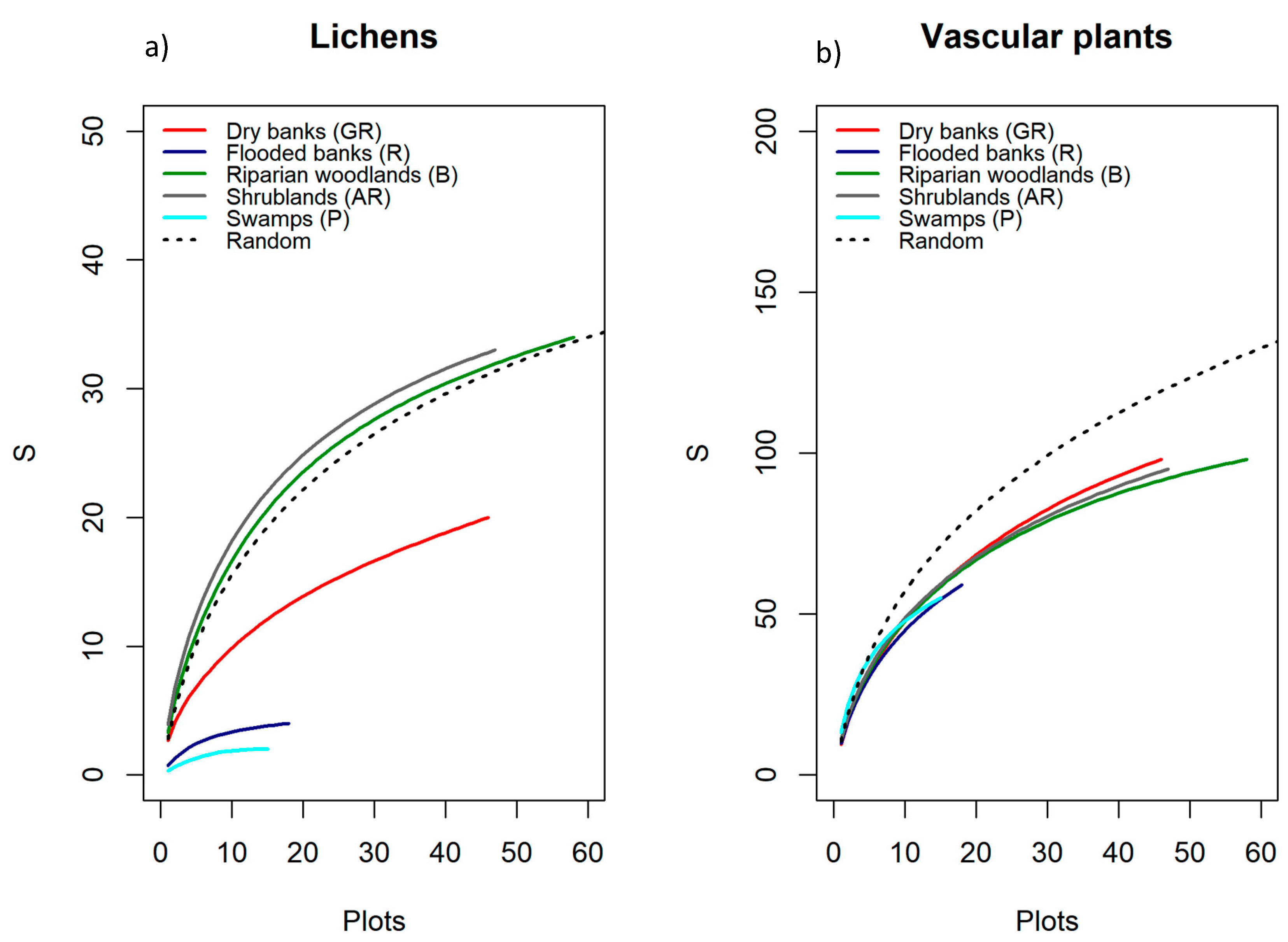
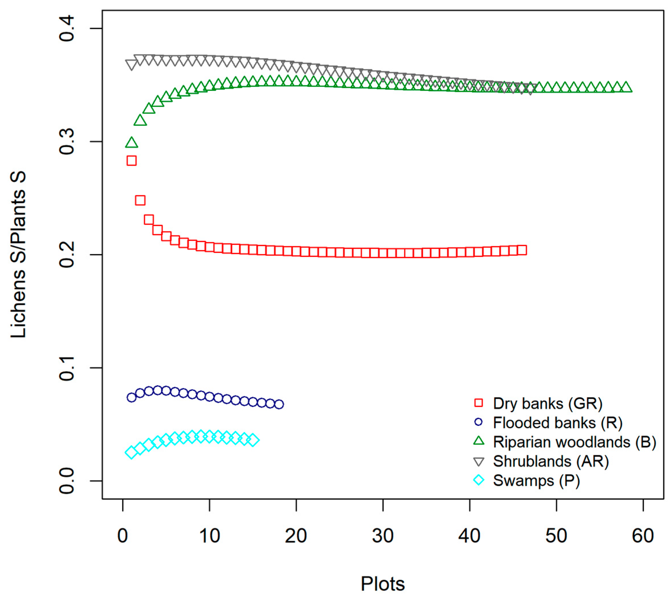
As pointed out by the cross-taxon correlation analysis we carried out between lichens and vascular plants richness, although the relationship resulted significant and positive in one of the five surveyed habitats (AR, shrublands) and negative in another one (P, Swamps), the overall performance of plant species richness per se as biodiversity surrogates of lichens was poor. Researchers working in various regions and using coarse grain plots (e.g., 50 × 50 m) obtained similar results and did not find any co-variation between the species richness of vascular plants and lichens [36,77]. In our study, many factors may have contributed to the general lack of species richness congruence and, among these, the small grain of the sampling units (1 m2) may be considered one of them. Additionally, the functional characteristics of a particular taxon could be another factor affecting the degree of concordance among different taxonomic groups, along with the life history of the site. For instance, McMullin & Wiersma [80] recently pointed out that the relative richness and abundance of lichens can be effective indicators of forest continuity and diversity. In this study, the surveyed habitats are riparian woods and shrublands, which are not characterized by mature stands. Though lichens can rely only on these trees and shrubs as stable substrata to develop their thalli and build communities richer in species abundance and diversity than in the other three habitat types, lichen diversity is still limited.
In assessing congruence patterns, species richness has been often used instead of species composition considering it is much simpler and faster to collect in the field. In surrogacy studies, it is often discussed whether it is reasonable to use species richness of vascular plants as a proxy of total biodiversity [39,42,81,82], even though different patterns of co-variation in lichen composition are described in relation to the variation of composition of plants communities. Our results also confirm the role of methodological issues, such as the type of data used (presence/absence vs. abundances) in determining the strength of cross-taxon relationships. Specifically, we observed that the degree of congruence in compositional patterns between lichens and vascular plants can substantially vary across habitats and depends on the type of the data used, along with the characteristic of the vegetation (abundance vs. presence/absence). Recent studies showed how the use of two-three taxa instead of a single one may drastically increase surrogacy [83].

4.2. Congruence in Species Composition

In general, our findings describe different patterns of co-variation in lichen composition in relation to the composition variation of plants communities. Our results also confirm the role of methodological issues such as the type of data used (presence/absence vs. abundances) in determining the strength of cross-taxon relationships. Specifically, we observed that the degree of congruence in compositional patterns between lichens and vascular plants can substantially vary across habitats and depends on the type of the data used, along with the characteristic of the vegetation (abundance vs. presence/absence data, species composition vs. variation in habitat characteristics). As for analysis at the species richness level discussed above, we showed a strong spatial structure of the data, which is also related to the spatial scale of the analysis. Specifically, at a coarser scale (i.e., along the ecological gradient), where environmental and structural gradients are more pronounced, especially for plant communities, these relationships display the strongest and clearest direction. On the other hand, at a finer scale, this signal seems to be hampered (see Table 3).
Nonetheless, studies at smaller grains (e.g., 1 × 1 m) have shown relatively strong correlations between vascular plants and lichens (see, for instance [71,84]). In general, our results corroborate previous evidence, especially those concerning the covariation in plant and lichen composition along the whole transitional gradient from river-to-land. In fact, it is well-known that the configuration and heterogeneity of habitats (e.g., variation in habitat types) of an area strongly influences the number of species found in that area [85]. Structurally complex and more mature habitats, indeed, provide more niches and diverse ways of exploiting the environmental resources, thus increasing species diversity [86]. However, a weak degree of association in community composition of vascular plants and cryptogams was evidenced in other studies from Australian [36], Canadian [84], and New Zealand forests [87] and dry grasslands in Sweden [88]. In relation to our data, a previous study pointed out that the five habitats can be well defined and characterized using plant communities [46]. The habitats host a specific set of plants, each with defined functional and structural features. Furthermore, our findings suggested a low compositional similarity, both among and within sampling units collected in the five habitats (see
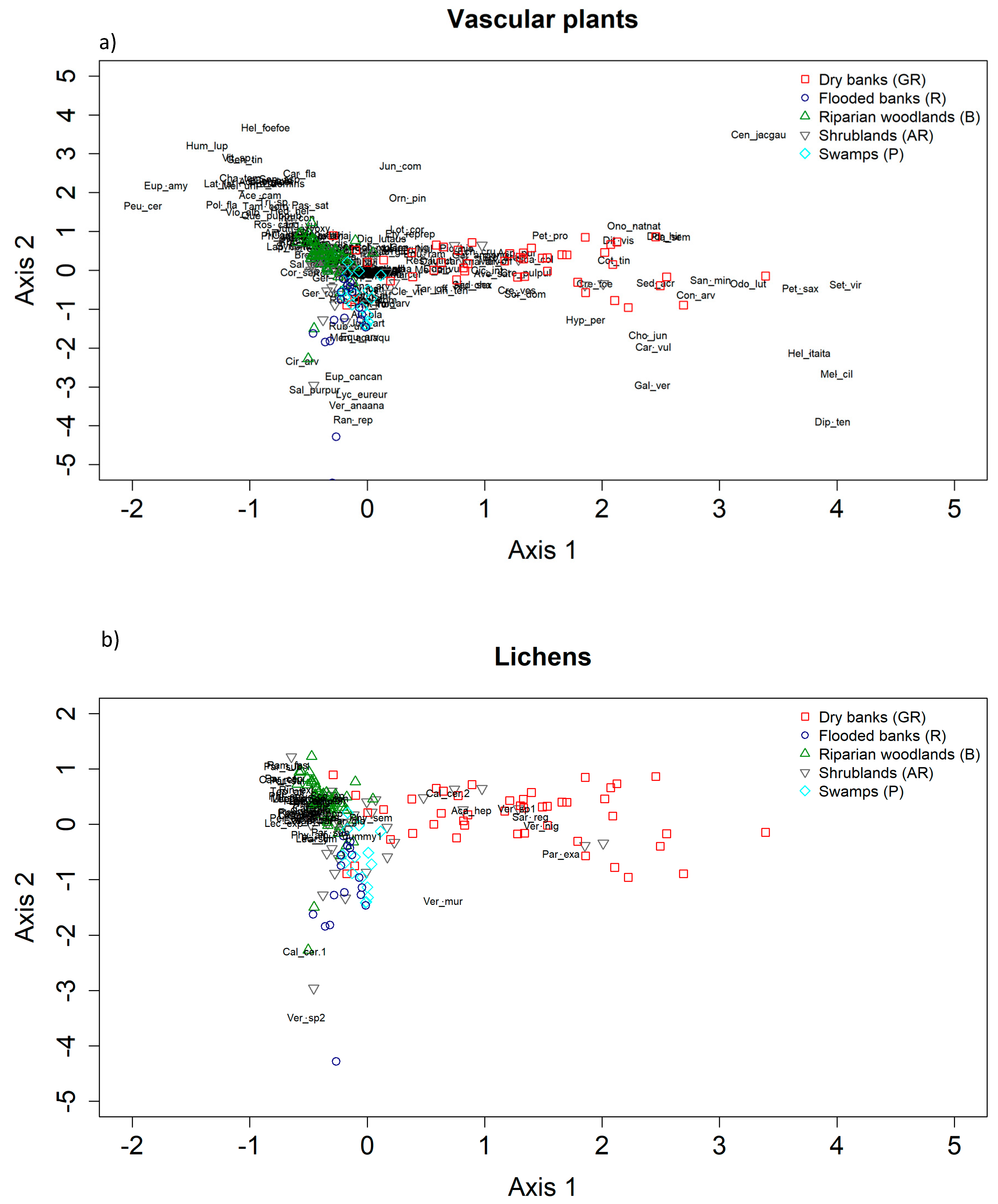
 Table 5 and Table 6). Based on these marked compositional differences, results of the Co-CA highlighted clear ordination patterns, as follows: For vascular plants, the marshlands indicator species group (P) is constituted mostly of water-related taxa, such as hydrophytes (Potamogeton nodosus), helophytes, or hygrophilous species (Typha minima, Alisma plantago–aquatica, Epipactis palustris, Scirpoides holoschoenus, Lythrum salicaria, Lycopus europaeus). Here, the few lichen species which are present are not exclusive to this habitat and are not represented at all in the Co-CA regions identified by (P) plots. The indicator species of the flooded banks (R) are mostly plants requiring a high ground water content (Mentha aquatica, Veronica anagallis–aquatica), species of cool and shaded habitats of the riparian forest fringes (Petasites hybridus, Senecio aquaticus, Schedonorus giganteus), or species resistant to trampling (Agrostis stolonifera, Prunella vulgaris). In this habitat, the recorded lichen species are those colonizing rocks, as the more stable substrate, and are mainly represented by the genus Verrucaria, which is known to comprehend amphibian taxa of both fresh and salt water and to develop thin partially or completely endolithic thalli.
The floristic component characterizing the dry banks (GR) is instead mostly composed of xerophilous vascular plant species such as Bromus erectus, Sanguisorba minor, Ononis natrix, Plantago sempervirens, and Scabiosa columbaria. These species are not strictly linked to the presence of water and indicate habitual long emersion times, which clearly differentiates this type of environment. Due to the instability of the substrate, characterized by sandy soil and pebbles, and the lack of shrubs or trees as substrate, the lichen communities are species poor and only few epilithic taxa were mainly surveyed, such as Sargogye regularis and Verrucaria spp.
The indicator species of riparian woods (B) are mostly trees which characterize the physiognomy of this habitat (Populus nigra and Alnus glutinosa) and a large number of shrubs, such as Cornus sanguinea, Ligustrum vulgare, Fraxinus ornus, and Rubus caesius. The presence of the invasive alien species Robinia pseudoacacia is also particularly significant [46]. Here, instead, lichens are mainly represented by epiphytic species, among which the few more generalist, nitrophilous taxa, such as Xanthoria parietina, Lecidella elaeochroma, and Lecanora hagenii, are frequently recorded.
A general consideration of the collected lichens relies on the fact that foliose macrolichens, such as those represented by the genera Parmelia and Ramalina, have been seldom surveyed across the five habitats. This might likely be due to the young forest/shrubs stands, in which the large foliose lichens did not have still time to develop conspicuously. The surveyed communities are mainly characterized by crustose species, which easily develop on the rather smooth bark of the tree and shrub species, such as those of the genera Lecanora, Lecidella, and Calopaca.
Finally, in our analysis we observed that the degree of cross-taxon congruence in species composition does not change strongly, regardless of the type of predictor variable used (abundance vs. presence/absence). Although it has been suggested that abundance data provide relatively detailed information concerning composition and structure of the communities [19,89], the collection of this type of data is labour and cost intensive. On other hand, the presence/absence data are less precise but much more cost effective. Our results showed that presence/absence data, for almost all the selected methodologies, provided similar results than those achieved by using abundances even if, on average, relationships were strongest when abundances were considered [19,90].

5. Conclusions

Recently, a new impulse to the study of cross-taxon relationship has been promoted, especially for nature conservation purposes [91]. Monitoring programs often use plants as general indicators of the conservation status of habitats, though plant species richness may be a poor indicator for the richness of other species groups, as also demonstrated and discussed above. Nevertheless, the use of plants in this context may represent a cost-effective approach to estimate environmental conditions [90,92] and habitat quality [93]. Our study strengthens the idea that cross-taxon congruence between plants and lichens is strongly habitat dependent. For sure it may provide useful information for biodiversity managers, although its use in real conservation contexts is far to be reliable. In conclusion, as emerged from this study, a stand-alone vegetation-driven conservation planning approach is likely to be ineffective to protect lichens diversity overall. In order to be effective, a detailed habitat-based assessment should be performed. This study then confirmed that cross-taxon congruence patterns are highly complex; thus, it is crucial to increase the spatial scale of the observations along with performing taxon-specific assessments.

Author Contributions

G.B. and L.L. conceived of the presented idea. E.T. performed computations. S.M. (Simona Maccherini) and M.M. verified the analytical methods. LL, T.G., R.B., V.G. collected the data, D.D.R., R.N., F.P., S.M. (Stefano Martellos), L.M. discussed the results and contributed to the final manuscript.

Funding

This research received no external funding.

Conflicts of Interest

The authors declare no conflict of interest.

Appendix A

Table A1. Abbreviation list of Lichens and Vascular Plants, as presented in the Co-Correspondence analysis (Fig. IV, Bacaro et al. 2019).
LichensVascular plants
SpeciesAbbr.SpeciesAbbr.
Acarospora heppiAca_hepAcer campestreAce_cam
Arthrosporum populorumArt_popAcer opalus subsp. obtusatumAce_opaobt
Caloplaca cerinaCal_cerAchillea millefoliumAch_mil
Caloplaca cerinellaCal_cer.1Aegopodium podagrariaAeg_pod
Caloplaca cfr. cerinelloidesCal_cer.2Agrimonia eupatoriaAgr_eup
Caloplaca pyraceaCal_pyrElymus caninusEly_can
Candelaria concolorCan_conElymus repens subsp. repensEly_reprep
Candelariella reflexaCan_refAgrostis stoloniferaAgr_sto
Candelariella xanthostigmaCan_xanAjuga chamaepitysAju_cha
Evernia prunastriEve_pruAlisma plantago-aquaticaAli_pla
Graphys o Arthonia cfr.Gra_cfrAlnus cordataAln_cor
Hyperphyscia adglutinataHyp_adgAlnus glutinosaAln_glu
Lecanora carpineaLec_carAmorpha fruticosaAmo_fru
Lecanora cfr. expallensLec_expAnagallis arvensisAna_arv
Lecanora chlaroteraLec_chlAnagallis foeminaAna_foe
Lecanora hageniiLec_hagCota tinctoriaCot_tin
Lecanora symmictaLec_symAnthyllis vulnerariaAnt_vul
Lecidella elaeocromaLec_elaHelosciadium nodiflorumHel_nod
Lepraria sp.Lep_sp.Artemisia vulgarisArt_vul
Micarea cfr. prasinaMic_praAsperula purpureaAsp_pur
Parmelia caperataPar_capAvena sativaAve_sat
Parmelia glabratulaPar_glaBarbarea vulgarisBar_vul
Parmelia subauriferaPar_subBidens frondosaBid_fro
Parmelia subrudectaPar_sub.1Bidens tripartitaBid_tri
Parmelia sulcataPar_sulBrachypodium rupestreBra_rup
Parmelia tiliaceaPar_tilBrachypodium sylvaticumBra_syl
Pertusaria albescensPer_albBromus erectusBro_ere
Phaeophyscia orbicularisPha_orbBromus madritensisBro_mad
Phlyctis argenaPhl_argCalystegia sepium subsp. sepiumCal_sepsep
Physcia adscendensPhy_adsCarex hirtaCar_hir
Physcia aipoliaPhy_aipCarex distansCar_dis
Physcia semipinnataPhy_semCarex flaccaCar_fla
Physconia distorta cfr.Phy_disCarex otrubaeCar_otr
Ramalina fastigiataRam_fasCarex pendulaCar_pen
Ramalina sp.Ram_sp.Carlina corymbosaCar_cor
Rinodina exiguaRin_exiCarlina vulgarisCar_vul
Sarcogine regularisSar_regCatapodium rigidumCat_rig
Scoliciosporum sp.Sco_sp.Centaurea jacea subsp. gaudiniCen_jacgau
Tephromela atraTep_atrCentaurea nigrescensCen_nig
Verrucaria cfr. muralisVer_murCephalaria transsylvanicaCep_tra
Verrucaria nigrescensVer_nigChaerophyllum temulumCha_tem
Verrucaria tallo continuo marroneVer_sp1Chara vulgarisCha_vul
Verrucaria tallo nero acquaticaVer_sp2Chondrilla junceaCho_jun
Xanthoria parietinaXan_parCichorium intybusCic_int
Parmelia exasperataPar_exaCirsium arvenseCir_arv
Cirsium creticum subsp. triumfettiCir_cretri
Cirsium vulgareCir_vul
Clematis vitalbaCle_vit
Colutea arborescensCol_arb
Convolvulus arvensisCon_arv
Cornus sanguineaCor_san
Emerus major subsp. majorEme_majmaj
Corylus avellanaCor_ave
Crepis foetidaCre_foe
Crepis pulchra subsp. pulchraCre_pulpul
Crepis vesicariaCre_ves
Cruciata glabraCru_gla
Cruciata laevipesCru_lae
Dactylis glomerataDac_glo
Daucus carotaDau_car
Digitalis lutea subsp. australisDig_lutaus
Diplotaxis tenuifoliaDip_ten
Dorycnium hirsutumDor_hir
Echinochloa crusgalliEch_cru
Echium vulgareEch_vul
Epilobium hirsutumEpi_hir
Epipactis cfr. helleborineEpi_hel
Epipactis palustrisEpi_pal
Equisetum arvenseEqu_arv
Equisetum palustreEqu_pal
Equisetum ramosissimumEqu_ram
Eupatorium cannabinum subsp. cannabinumEup_cancan
Euphorbia amygdaloidesEup_amy
Euphorbia platyphillosEup_pla
Schenodorus arundinaceusSch_aru
Schedonorus giganteusSch_gig
Fontinalis antipyreticaFon_ant
Fraxinus ornus subsp. ornusFra_ornorn
Galega officinalisGal_off
Galeopsis angustifolia subsp. angustifoliaGal_angang
Galium mollugo subsp. erectumGal_molere
Galium aparineGal_apa
Galium palustre subsp. palustreGal_palpal
Galium verumGal_ver
Genista tinctoriaGen_tin
Geranium columbinumGer_col
Geranium robertianumGer_rob
Geranium rotundifoliumGer_rot
Hedera helixHed_hel
Helichrysum italicum subsp. italicumHel_itaita
Helleborus bocconei subsp. bocconeiHel_bocboc
Helleborus foetidus subsp. foetidusHel_foefoe
Humulus lupulusHum_lup
Hypericum perforatumHyp_per
Inula conyzaeInu_con
Dittrichia viscosaDit_vis
Juglans regiaJug_reg
Juncus articulatusJun_art
Juncus fontanesii subsp. fontanesiiJun_fonfon
Juncus inflexusJun_inf
Juniperus communisJun_com
Juniperus oxycedrus subsp. oxycedrusJun_oxyoxy
Knautia arvensisKna_arv
Lapsana communis subsp. communisLap_comcom
Lathyrus latifoliusLat_lat
Lathyrus sylvestris subsp. sylvestrisLat_sylsyl
Leucanthemum vulgare subsp. vulgareLeu_vulvul
Ligustrum vulgareLig_vul
Linum tenuifoliumLin_ten
Lonicera etruscaLon_etr
Lotus corniculatusLot_cor
Lycopus europaeus subsp. europaeusLyc_eureur
Lysimachia nummulariaLys_num
Lythrum salicariaLyt_sal
Melica ciliataMel_cil
Melica unifloraMel_uni
Melilotus albusMel_alb
Melilotus officinalisMel_off
Mentha aquatica subsp. aquaticaMen_aquaqu
Mentha spicataMen_spi
Molinia caerulea subsp. arundinaceaMol_caearu
Nasturtium officinale subsp. officinaleNas_offoff
Odontites luteusOdo_lut
Odontites vulgarisOdo_vul
Ononis natrix subsp. natrixOno_natnat
Ornithopus pinnatusOrn_pin
Pastinaca sativaPas_sat
Petasites hybridus subsp. hybridusPet_hybhyb
Petrorhagia proliferaPet_pro
Petrorhagia saxifragaPet_sax
Peucedanum cervariaPeu_cer
Peucedanum verticillarePeu_ver
Helminthotheca echioidesHel_ech
Picris hieracioidesPic_hie
Plantago sempervirensPla_sem
Plantago lanceolataPla_lan
Plantago majorPla_maj
Poa compressaPoa_com
Polygala flavescensPol_fla
Persicaria maculosaPer_mac
Populus albaPop_alb
Populus nigraPop_nig
Potamogeton nodosusPot_nod
Potentilla reptansPot_rep
Primula vulgaris subsp. vulgarisPri_vulvul
Prunella vulgaris subsp. vulgarisPru_vulvul
Prunus avium subsp. aviumPru_aviavi
Prunus domestica subsp. domesticaPru_domdom
Prunus domestica subsp. insititiaPru_domins
Prunus spinosa subsp. spinosaPru_spispi
Pulicaria dysentericaPul_dys
Quercus cerrisQue_cer
Quercus pubescens subsp. pubescensQue_pubpub
Ranunculus lanuginosusRan_lan
Ranunculus repensRan_rep
Reseda lutea subsp. luteaRes_lutlut
Robinia pseudacaciaRob_pse
Rosa caninaRos_can
Rubus caesiusRub_cae
Rubus ulmifoliusRub_ulm
Salix albaSal_alb
Salix eleagnos subsp. eleagnosSal_eleele
Salix purpurea subsp. purpureaSal_purpur
Salix triandraSal_tri
Sanguisorba minorSan_min
Scabiosa columbariaSca_col
Schoenus nigricansSch_nig
Scirpoides holoschoenusSci_hol
Scrophularia caninaScr_can
Sedum acreSed_acr
Sedum sexangulareSed_sex
Senecio aquaticusSen_aqu
Setaria viridisSet_vir
Solanum dulcamaraSol_dul
Sonchus arvensisSon_arv
Sonchus asperSon_asp
Sorbus domesticaSor_dom
Sparganium erectum subsp. erectumSpa_ereere
Spartium junceumSpa_jun
Succisa pratensisSuc_pra
Symphytum tuberosum subsp. angustifoliumSym_tubang
Tamus communisTam_com
Taraxacum gr. officinaleTar_off
Thalictrum flavumTha_fla
Torilis arvensisTor_arv
Trifolium sp.Tri_sp.
Tussilago farfaraTus_far
Typha minimaTyp_min
Ulmus minorUlm_min
Verbascum thapsus subsp. thapsusVer_thatha
Veronica anagallis-aquatica subsp. anagallis-aquaticaVer_anaana
Viola albaVio_alb
Vitis sp.Vit_sp.

References

  1. Colwell, R.K.; Coddington, J.A. Estimating terrestrial biodiversity through extrapolation. Philos. Trans. R. Soc. Lond. B Biol. Sci. 1994, 345, 101–118. [Google Scholar] [CrossRef] [PubMed] [Green Version]
  2. Harper, J.L.; Hawksworth, D. Biodiversity: Measurement and Estimation. Philos. Trans. R. Soc. Lond. B Biol. Sci. 1994, 345, 5–12. [Google Scholar] [CrossRef] [PubMed]
  3. Gaston, K.J. Global patterns in biodiversity. Nature 2000, 405, 220. [Google Scholar] [CrossRef] [PubMed]
  4. Kati, V.; Devillers, P.; Dufrêne, M.; Legakis, A.; Vokou, D.; Lebrun, P. Testing the value of six taxonomic groups as biodiversity indicators at a local scale. Conserv. Biol. 2004, 18, 667–675. [Google Scholar] [CrossRef]
  5. Rocchini, D.; Bacaro, G.; Chirici, G.; Da Re, D.; Feilhauer, H.; Foody, G.M.; Galluzzi, M.; Garzon-Lopez, C.X.; Gillespie, T.W.; He, K.S.; et al. Remotely sensed spatial heterogeneity as an exploratory tool for taxonomic and functional diversity study. Ecol. Indic. 2018, 85, 983–990. [Google Scholar] [CrossRef] [Green Version]
  6. Westgate, M.J.; Barton, P.S.; Lane, P.W.; Lindenmayer, D.B. Global meta-analysis reveals low consistency of biodiversity congruence relationships. Nat. Commun. 2014, 5, 3899. [Google Scholar] [CrossRef] [PubMed] [Green Version]
  7. Sarkar, S.; Margules, C. Operationalizing biodiversity for conservation planning. J. Biosci. 2002, 27, 299–308. [Google Scholar] [CrossRef] [PubMed]
  8. Pearson, D.L.; Carroll, S.S. The influence of spatial scale on cross-taxon congruence patterns and prediction accuracy of species richness. J. Biogeogr. 1999, 26, 1079–1090. [Google Scholar] [CrossRef]
  9. Jackson, D.A.; Harvey, H.H. Fish and benthic invertebrates: Community concordance and community–environment relationships. Can. J. Fish. Aquat. Sci. 1993, 50, 2641–2651. [Google Scholar] [CrossRef]
  10. Ter Braak, C.J.F.; Schaffers, A.P. Co-correspondence analysis; a new ordination method to relate two species compositions. Ecology 2004, 85, 834–846. [Google Scholar] [CrossRef]
  11. Rooney, C.R.; Azeria, E.T. The strength of cross-taxon congruence in species composition varies with the size of regional species pools and the intensity of human disturbance. J. Biogeogr. 2015, 42, 439–451. [Google Scholar] [CrossRef]
  12. Brunbjerg, A.K.; Bruun, H.H.; Dalby, L.; Fløjgaard, C.; Frøslev, T.G.; Høye, T.T.; Goldberg, I.; Læssøe, T.; Hansen, M.D.D.; Brøndum, L.; et al. Vascular plant species richness and bioindication predict multi-taxon species richness. Methods Ecol. Evol. 2018, 9, 2372–2382. [Google Scholar] [CrossRef]
  13. Rodrigues, A.S.; Brooks, T.M. Shortcuts for biodiversity conservation planning: The effectiveness of surrogates. Annu. Rev. Ecol. Evol. Syst. 2007, 38, 713–737. [Google Scholar] [CrossRef]
  14. Prendergast, J.R.; Quinn, R.M.; Lawton, J.H.; Eversham, B.C.; Gibbons, D.W. Rare species, the coincidence of diversity hotspots and conservation strategies. Nature 1993, 365, 335–337. [Google Scholar] [CrossRef]
  15. Paszkowski, C.A.; Tonn, W.M. Community concordance between the fish and aquatic birds of lakes in northern Alberta, Canada: The relative importance of environmental and biotic factors. Freshw. Biol. 2000, 43, 421–437. [Google Scholar] [CrossRef]
  16. Chiarucci, A.; Bacaro, G.; Filibeck, G.; Landi, S.; Maccherini, S.; Scoppola, A. Scale dependence of plant species richness in a network of protected areas. Biodivers. Conserv. 2012, 21, 503–516. [Google Scholar] [CrossRef]
  17. Warman, L.D.; Forsyth, D.M.; Sinclair, A.R.E.; Freemark, K.; Moore, H.D.; Barrett, T.W.; Pressey, R.L.; White, D. Species distributions, surrogacy, and important conservation regions in Canada. Ecol. Lett. 2004, 7, 374–379. [Google Scholar] [CrossRef]
  18. Gioria, M.; Bacaro, G.; Feehan, J. Evaluating and interpreting cross-taxon congruence: Potential pitfalls and solutions. Acta Oecol. 2011, 37, 187–194. [Google Scholar] [CrossRef]
  19. Santi, E.; Bacaro, G.; Rocchini, D.; Chiarucci, A.; Bonini, I.; Brunialti, G.; Muggia, L.; Maccherini, S. Methodological issues in exploring cross-taxon congruence across vascular plants, bryophytes and lichens. Folia Geobot. 2016, 51, 297–304. [Google Scholar] [CrossRef]
  20. Jelinski, D.E.; Wu, J. The modifiable areal unit problem and implications for landscape ecology. Landsc. Ecol. 1996, 11, 129–140. [Google Scholar] [CrossRef]
  21. Paavola, R.; Muotka, T.; Virtanen, R.; Heino, J.; Kreivi, P. Are biological classifications of headwater streams concordant across multiple taxonomic groups? Freshw. Biol. 2003, 48, 1912–1923. [Google Scholar] [CrossRef]
  22. Santi, E.; Mari, E.; Piazzini, S.; Renzi, M.; Bacaro, G.; Maccherini, S. Dependence of animal diversity on plant diversity and environmental factors in farmland ponds. Community Ecol. 2010, 11, 232–241. [Google Scholar] [CrossRef]
  23. Howard, P.C.; Viskanic, P.; Davenport, T.R.B.; Kigenyi, F.W.; Baltzer, M.; Dickinson, C.J.; Lwanga, J.S.; Matthews, R.A.; Balmford, A. Complementarity and the use of indicator groups for reserve selection in Uganda. Nature 1998, 394, 472–475. [Google Scholar] [CrossRef]
  24. Gaston, K.J.; Williams, P.H. Spatial patterns in taxonomic diversity. In Biodiversity: A Biology of Numbers and Difference; Gaston, K.J., Ed.; Blackwell Science Ltd.: Oxford, UK, 1996; pp. 202–229. [Google Scholar]
  25. Heino, J. Are indicator groups and cross-taxon congruence useful for predicting biodiversity in aquatic ecosystems? Ecol. Indic. 2009, 10, 112–117. [Google Scholar] [CrossRef]
  26. Noss, R.F. Indicators for monitoring biodiversity: A hierarchical approach. Conserv. Biol. 1990, 4, 355–364. [Google Scholar] [CrossRef]
  27. Pearson, D.L. Selecting indicator taxa for the quantitative assessment of biodiversity. Philos. Trans. R. Soc. Lond. B Biol. Sci. 1994, 345, 75–79. [Google Scholar] [CrossRef] [PubMed]
  28. Ryti, R.T. Effect of the focal taxon on the selection of nature reserves. Ecol. Appl. 1992, 2, 404–410. [Google Scholar] [CrossRef] [PubMed]
  29. Marignani, M.; Blasi, C. Looking for Important Plant Areas: Selection based on criteria, complementarity, or both? Biodivers. Conserv. 2012, 21, 853–1864. [Google Scholar] [CrossRef]
  30. Marignani, M.; Bruschi, D.; Astiaso Garcia, D.; Frondoni, R.; Carli, E.; Pinna, M.S.; Cumo, F.; Gugliermetti, F.; Saatkamp, A.; Doxa, A.; et al. Identification and prioritization of areas with high environmental risk in Mediterranean coastal areas: A flexible approach. Sci. Total Environ. 2017, 590, 566–578. [Google Scholar] [CrossRef]
  31. Carli, E.; Frondoni, R.; Pinna, M.S.; Bacchetta, G.; Fenu, G.; Fois, M.; Marignani, M.; Puddu, S.; Blasi, C. Spatially assessing plant diversity for conservation: A Mediterranean case study. J. Nat. Conserv. 2018, 41, 35–43. [Google Scholar] [CrossRef]
  32. Pharo, E.J.; Beattie, A.J.; Pressey, R.L. Effectiveness of using vascular plants to select reserves for bryophytes and lichens. Biol. Conserv. 2000, 96, 371–378. [Google Scholar] [CrossRef]
  33. Bacaro, G.; Baragatti, E.; Chiarucci, A. Using taxonomic data to assess and monitor biodiversity: Are the tribes still fighting? J. Environ. Monit. 2009, 11, 798–801. [Google Scholar] [CrossRef] [PubMed]
  34. Santi, E.; Maccherini, S.; Rocchini, D.; Bonini, I.; Brunialti, G.; Favilli, L.; Perini, C.; Pezzo, F.; Piazzini, S.; Rota, E.; et al. Simple to sample: Vascular plants as surrogate group in a nature reserve. J. Nat. Conserv. 2010, 18, 2–11. [Google Scholar] [CrossRef]
  35. Gao, T.; Nielsen, A.B.; Hedblom, M. Reviewing the strength of evidence of biodiversity indicators for forest ecosystems in Europe. Ecol. Indic. 2015, 57, 420–434. [Google Scholar] [CrossRef]
  36. Pharo, E.J.; Beattie, A.J.; Binns, D. Vascular plants diversity as a surrogate for bryophyte and lichen diversity. Biol. Conserv. 1999, 13, 282–292. [Google Scholar] [CrossRef]
  37. Sætersdal, M.; Gjerde, I.; Blom, H.H.; Ihlen, P.G.; Myrseth, E.W.; Pommeresche, R.; Skartveit, J.; Solhøy, T.; Aas, O. Vascular plants as a surrogate species group in complementary site selection for bryophytes, macrolichens, spiders, carabids, staphylinids, snails, and wood living polypore fungi in a northern forest. Biol. Conserv. 2004, 115, 21–31. [Google Scholar] [CrossRef]
  38. Jokela, J.; Juutilainen, K.; Korpela, L.; Kouki, J.; Kuntsi, S.; Koivula, M.; Siitonen, J. Cross-taxon congruence and relationships to stand characteristics of vascular plant, bryophytes, polyporous fungi and beetles in mature managed boreal forests. Ecol. Indic. 2018, 85, 137–145. [Google Scholar] [CrossRef]
  39. Burrascano, S.; de Andreade, R.B.; Paillet, Y.; Odor, P.; Antonini, G.; Bouget, C.; Campagnaro, T.; Gosselin, F.; Janssen, P.; Persiani, A.M.; et al. Congruence across taxa and spatial scales: Are we asking too much of species data? Glob. Ecol. Biogeogr. 2018, 27, 980–990. [Google Scholar] [CrossRef]
  40. Chiarucci, A.; D’auria, F.; Bonini, I. Is vascular plant species diversity a predictor of bryophyte species diversity in Mediterranean forests? Biodivers. Conserv. 2007, 16, 525–545. [Google Scholar] [CrossRef]
  41. Maccherini, S.; Santi, E.; Bonini, I.; Amici, V.; Pruscini, S.; Palazzo, D.; Selva, F.C. The impact of land abandonment on the plant diversity of olive groves. Biodivers. Conserv. 2013, 22, 3067–3083. [Google Scholar] [CrossRef]
  42. Maccherini, S.; Bacaro, G.; Favilli, L.; Piazzini, S.; Santi, E.; Marignani, M. Congruence among vascular plants and butterflies in the evaluation of grassland restoration success. Acta Oecol. 2009, 35, 311–317. [Google Scholar] [CrossRef]
  43. Nascimbene, J.; Marini, L.; Nimis, P.L. Epiphytic lichens in a riparian natural reserve of Northen Italy: Species richness, composition and conservation. Plant Biosyst. 2008, 142, 94–98. [Google Scholar] [CrossRef]
  44. Naiman, R.J.; Décamps, H. The ecology of interfaces: Riparian zones. Annu. Rev. Ecol. Syst. 1997, 28, 621–658. [Google Scholar] [CrossRef]
  45. Poff, B.; Koestner, K.A.; Neary, D.G.; Henderson, V. Threats to Riparian Ecosystems in Western North America: An Analysis of Existing Literature. J. Am. Water Resour. Assoc. 2011, 47, 1241–1254. [Google Scholar] [CrossRef]
  46. Lastrucci, L.; Lazzaro, L.; Guidi, T.; Gonnelli, V.; Giordani, P.; Benesperi, R. Different components of plant diversity suggest the protection of a large area for the conservation of a riparian ecosystem. Biologia 2015, 70, 1033–1041. [Google Scholar] [CrossRef]
  47. Lastrucci, L.; Raffaelli, M. Contribution to the knowledge of the floodplains and hilly wetlands of eastern Tuscany: The district of Arezzo (central Italy). Webbia 2006, 61, 271–304. [Google Scholar] [CrossRef]
  48. Conti, F.; Abbate, G.; Alessandrini, A.; Blasi, C. (Eds.) An Annotated Checklist of the Italian Vascular Flora; Palombi Editori: Roma, Italy, 2005. [Google Scholar]
  49. Nimis, P.L.; Martellos, S. A Second Checklist of the Lichens of Italy, with a Thesaurus of Synonyms; Museo Regionale di Scienze Naturali: Torino, Italy, 2003; pp. 1–192. [Google Scholar]
  50. Gotelli, N.J.; Colwell, R.K. Quantifying biodiversity: Procedures and pitfalls in the measurement and comparison of species richness. Ecol. Lett. 2001, 4, 379–391. [Google Scholar] [CrossRef]
  51. Kobayashi, S. The species-area relation I. A model for discrete sampling. Res. Popul. Ecol. 1973, 15, 223–237. [Google Scholar] [CrossRef]
  52. Chiarucci, A.; Bacaro, G.; Rocchini, D.; Fattorini, L. Discovering and rediscovering the rarefaction formula in ecological literature. Community Ecol. 2008, 9, 121–123. [Google Scholar] [CrossRef]
  53. Bacaro, G.; Rocchini, D.; Ghisla, A.; Marcantonio, M.; Neteler, M.; Chiarucci, A. The spatial domain matters: Spatially constrained species rarefaction in a Free and Open source environment. Ecol. Complex. 2012, 12, 63–69. [Google Scholar] [CrossRef]
  54. Bacaro, G.; Altobelli, A.; Cameletti, M.; Ciccarelli, D.; Martellos, S.; Palmer, M.W.; Ricotta, C.; Rocchini, D.; Scheiner, S.M.; Tordoni, E.; et al. Incorporating spatial autocorrelation in rarefaction methods: Implications for ecologists and conservation biologists. Ecol. Indic. 2016, 69, 233–238. [Google Scholar] [CrossRef] [Green Version]
  55. Tordoni, E.; Napolitano, R.; Nimis, P.; Castello, M.; Altobelli, A.; Da Re, D.; Zago, S.; Chines, A.; Martellos, S.; Maccherini, S.; et al. Diversity patterns of alien and native plant species in Trieste port area: Exploring the role of urban habitats in biodiversity conservation. Urban Ecosyst. 2017, 20, 1151–1160. [Google Scholar] [CrossRef]
  56. Clarke, K.R. Non-parametric multivariate analyses of changes in community structure. Aust. J. Ecol. 1993, 18, 117–143. [Google Scholar] [CrossRef]
  57. Jackson, D.A. PROTEST: A PROcrustean Randomization TEST of community environment concordance. Écoscience 1995, 2, 297–303. [Google Scholar] [CrossRef]
  58. Manly, B.F.J. Randomization, Bootstrap and Monte Carlo Methods. In Biology, 2nd ed.; Chapman and Hall: London, UK, 1997. [Google Scholar]
  59. Legendre, P.; Legendre, L. Numerical Ecology, 3rd ed.; Elsevier Publishing: Amsterdam, The Netherlands, 2012; ISBN 9780444538680. [Google Scholar]
  60. Podani, J. Introduction to the Exploration of Multivariate Biological Data; Backhuys: Leiden, NL, USA, 2000. [Google Scholar]
  61. Schaffers, A.P.; Raemakers, I.P.; Sýkora, K.V.; ter Braak, C.J. Arthropod assemblages are best predicted by plant species composition. Ecology 2008, 89, 782–794. [Google Scholar] [CrossRef] [PubMed]
  62. Martens, H.; Næs, T. Multivariate Calibration; John Wiley and Sons: Hoboken, NJ, USA, 1992. [Google Scholar]
  63. Legendre, P.; Borcard, D.; Peres-Neto, P.R. Analyzing beta diversity: Partitioning the spatial variation of community composition data. Ecol. Monogr. 2005, 75, 435–450. [Google Scholar] [CrossRef]
  64. Whittaker, R.H. Evolution and measurement of species diversity. Taxon 1972, 21, 213–251. [Google Scholar] [CrossRef]
  65. Bacaro, G.; Gioria, M.; Ricotta, C. Testing for differences in beta diversity from plot-to-plot dissimilarities. Ecol. Res. 2012, 27, 285–292. [Google Scholar] [CrossRef]
  66. Bacaro, G.; Gioria, M.; Ricotta, C. Beta diversity reconsidered. Ecol. Res. 2013, 28, 537–540. [Google Scholar] [CrossRef]
  67. R Development Core Team. R: A Language and Environment for Statistical Computing; R Foundation for Statistical Computing: Vienna, Austria, 2018. [Google Scholar]
  68. Oksanen, J.; Blanchet, F.G.; Kindt, R.; Legendre, P.; O’Hara, R.G.; Simpson, G.L.; Solymos, P.; Henry, M.; Stevens, H.; Wagner, H. Vegan: Community Ecology Package; R Package Version 1.17-0. 2010. Available online: http://CRAN.R-project.org/ (accessed on 12/10/2018).
  69. Simpson, G.L. Cocorresp: Co-Correspondence Analysis Ordination Methods; R Package Version 0.3-0. 2009. Available online: http://cran.r-project.org/packa ge=analogue (accessed on 12/10/2018).
  70. Ricketts, T.H.; Dinerstein, E.; Olson, D.M.; Loucks, C. Who’s where in North America? Patterns of species richness and the utility of indicator taxa for conservation. BioScience 1999, 49, 369–381. [Google Scholar] [CrossRef]
  71. Negi, H.R.; Gadgil, M. Cross-taxon surrogacy of biodiversity in the Indian Garhwal Himalaya. Biol. Conserv. 2002, 105, 143–155. [Google Scholar] [CrossRef]
  72. Vessby, K.; Söderström, B.O.; Glimskär, A.; Svensson, B. Species-richness correlations of six different taxa in Swedish seminatural grasslands. Conserv. Biol. 2002, 16, 430–439. [Google Scholar] [CrossRef]
  73. Su, J.C.; Debinski, D.M.; Jakubauskas, M.E.; Kindscher, K. Beyond species richness: Community similarity as a measure of cross-taxon congruence for coarse-filter conservation. Conserv. Biol. 2004, 18, 167–173. [Google Scholar] [CrossRef]
  74. Similä, M.; Kouki, J.; Mönkkönen, M.; Sippola, A.; Huhta, E. Co-variation and indicators of species diversity: Can richness of forest-dwelling species be predicted in northern boreal forests? Ecol. Indic. 2006, 6, 686–700. [Google Scholar] [CrossRef]
  75. Schouten, M.A.; Verweij, P.A.; Barendregt, A.; Kleukers, R.M.J.C.; Kalkman, V.J.; De Ruiter, P.C. Determinants of species richness patterns in the Netherlands across multiple taxonomic groups. Biodivers Conserv. 2009, 18, 203–217. [Google Scholar] [CrossRef]
  76. Söderström, L. Distribution of bryophytes in spruce forests on hill slopes in central Sweden. Wahlenbergia Scr. Bot. Umensia 1981, 7, 141. [Google Scholar]
  77. Jonsson, B.G.; Jonsell, M. Exploring potential biodiversity indicators in boreal forests. Biodivers. Conserv. 1999, 8, 1417–1433. [Google Scholar] [CrossRef]
  78. Bradfield, G.E.; Scagel, A. Correlations among vegetation strata and environmental variables in subalpine spruce-fir forests, southeastern British Columbia. Vegetatio 1984, 55, 105–114. [Google Scholar] [CrossRef]
  79. Rey Benayas, J.M. Patterns of diversity in the strata of boreal montane forest in British Columbia. J. Veg. Sci. 1995, 6, 95–98. [Google Scholar] [CrossRef]
  80. McMullin, R.T.; Wiersma, Y. Out with OLD growth, in with ecological continNEWity: New perspectives on forest conservation. Front. Ecol. Environ. 2019, 17, 176–181. [Google Scholar] [CrossRef]
  81. Gioria, M.; Pyšek, P.; Moravcová, L. Soil seed banks in plant invasions: Promoting species invasiveness and long-term impact on plant community dynamics. Preslia 2012, 84, 327–350. [Google Scholar]
  82. Barbato, D.; Perini, C.; Mocali, S.; Bacaro, G.; Tordoni, E.; Maccherini, S.; Marchi, M.; Cantiani, P.; De Meo, I.; Bianchetto, E.; et al. Teamwork makes the dream work: Disentangling cross-taxon congruence across soil biota in black pine plantations. Sci. Total Environ. 2019, 656, 659–669. [Google Scholar] [CrossRef] [PubMed]
  83. Larrieu, L.; Gosselin, F.; Archaux, F.; Chevalier, R.; Corriol, G.; Dauffy-Richard, E.; Deconchat, M.; Gosselin, M.; Ladet, S.; Savoie, J.M.; et al. Cost-efficiency of cross-taxon surrogates in temperate forests. Ecol. Indic. 2018, 87, 56–65. [Google Scholar] [CrossRef]
  84. Anand, M.; Laurence, S.; Rayfield, B. Diversity relationship among taxonomic groups in recovering and restored forests. Conserv. Biol. 2005, 19, 955–962. [Google Scholar] [CrossRef]
  85. Chuquimarca, L.; Gaona, P.F.; Iñiguez-Armijos, C.; Benítez, A. Lichen Responses to Disturbance: Clues for Biomonitoring Land-use Effects on Riparian Andean Ecosystem. Diversity 2019, 11, 73. [Google Scholar] [CrossRef]
  86. Atauri, J.A.; De Lucio, J.V. The role of landscape structure in species richness distribution of birds, amphibians, reptiles and lepidopterans in Mediterranean landscapes. Landsc. Ecol. 2001, 16, 147–159. [Google Scholar] [CrossRef]
  87. Affeld, K.; Sullivan, J.; Worner, S.P.; Didham, R.K. Can spatial variation in epiphyte diversity and community structure be predicted from sampling vascular epiphytes alone? J. Biogeogr. 2008, 35, 2274–2288. [Google Scholar] [CrossRef]
  88. Löbel, S.; Dengler, J.; Hobohm, C. Species richness of vascular plants, bryophytes and lichens in dry grasslands: The effects of environment, landscape structure and competition. Folia Geobot. 2006, 41, 377–393. [Google Scholar] [CrossRef]
  89. Maccherini, S.; Bacaro, G.; Giovannetti, G.; Angiolini, C.; Chiarucci, A. Analysing methodological issues in short-term monitoring of rare European beech forests restoration. Plant Biosyst. 2019, 153, 60–67. [Google Scholar] [CrossRef]
  90. Cushman, A.S.; McGarigal, K. Patterns in the species–environment relationship depend on both scale and choice of response variables. Oikos 2004, 105, 117–124. [Google Scholar] [CrossRef]
  91. Uboni, C.; Tordoni, E.; Brandmayr, P.; Battistella, S.; Bragato, G.; Castello, M.; Colombetta, G.; Poldini, L.; Bacaro, G. Exploring cross-taxon congruence between carabid beetles (Coleoptera: Carabidae) and vascular plants in sites invaded by Ailanthus altissima versus non-invaded sites: The explicative power of biotic and abiotic factors. Ecol. Ind. 2019, 103, 145–155. [Google Scholar] [CrossRef]
  92. Diekmann, M. Species indicator values as an important tool in applied plant ecology—A review. Basic Appl. Ecol. 2003, 4, 493–506. [Google Scholar] [CrossRef]
  93. Andersen, D.K.; Nygaard, B.; Fredshavn, J.R.; Ejrnæs, R. Cost-effective assessment of conservation status of fens. Appl. Veg. Sci. 2013, 16, 491–501. [Google Scholar] [CrossRef] [Green Version]
Figure 1. Location of the study area. Sampled transects are drawn as black lines.
Diversity 11 00133 g001
Figure 2. (a,b) Plot-based rarefaction curves calculated for lichens (a) and vascular plants (b), recorded from 184 plots sampled along the Tiber river for each riparian vegetation habitat vegetation types, showing the expected number of species, S, as a function of the number of plots. The plot-based rarefaction curve for the pooled sample of all the 184 plots is also shown (dashed line).
Diversity 11 00133 g002
Figure 3. Ratio of lichens and plant rarefaction curves for the whole dataset and for each habitat explored separately.
Diversity 11 00133 g003
Figure 4. (a,b) Predictive Co-CA biplot of plant species composition (a) and lichen species composition (b) using abundance data. In each plot, species are positioned according to their loadings, with respect to normalized plot scores derived from the plant composition data. Symbols show the type of riparian vegetation habitat of each plot. The axes were rescaled to the same ranges so that sites occupy the same position in both plots. Explanations of species abbreviations are reported in Appendix A.
Diversity 11 00133 g004
Table 1. Summary statistics of the analyzed dataset.
TaxonN° Sampled PlotN° Sampled SpeciesMean Species RichnessMin–Max
Whole datasetPlants18419310.572–21
Lichens184452.790–15
Shrublands (AR)Plants479510.612–21
Lichens47333.910–15
Riparian woods (B)Plants589811.054–21
Lichens58343.290–12
Dry Banks (GR)Plants46989.363–17
Lichens46202.650–8
Swamps (P)Plants155513.23–21
Lichens1520.330–2
Flooded Banks (R)Plants18599.772–18
Lichens1840.720–4
Table 2. Spearman correlations (ρ) between plant and lichen species richness for the whole set of data and for each habitat separately. (** p < 0.01; * p < 0.05).
Dataρ
Whole Dataset0.050
Shrublands (AR)0.407 **
Riparian woods (B)0.208
Dry Banks (GR)0.011
Swamps (P)−0.587 *
Table 3. Correlation (Spearman’s ρ) between the Bray–Curtis (log-transformed abundance data) and Jaccard dissimilarity matrices (occurrence data) of plants and lichens. p-values were calculated by using Monte Carlo randomization tests (999 permutations). Significant correlation coefficients are in bold. AR—Shrublands, B—Riparian woods, GR—Dry Banks, P—Swamps, R—Flooded Banks.
DatasetDissimilarity Metricρp
Whole DatasetBray–Curtis0.238<0.001
Jaccard0.153<0.001
ARBray–Curtis0.349<0.001
Jaccard0.272<0.001
BBray–Curtis0.0880.007
Jaccard0.0390.171
GRBray–Curtis0.346<0.001
Jaccard0.2020.006
PBray–Curtis0.1950.088
Jaccard0.2670.052
RBray–Curtis0.2580.038
Jaccard0.3390.014
Table 4. Significance of Co-CA axes for lichens and plants considering both presence/absence and abundance data. Significant cross-validatory fit is shown in bold.
Co-CA ModelAxisCross-Validatory (%) Fitp
Presence/Absence data15.5280.01
25.4860.01
37.1720.06
46.9650.17
Abundance Data18.2700.01
25.9700.01
33.4720.06
42.5520.24
Table 5. Mean beta diversity measures calculated for plants and lichens, separately. AR—Shrublands, B—Riparian woods, GR—Dry Banks, P—Swamps, R—Flooded Banks.
DatasetDissimilarity MeasureAverage Beta Diversity LichensAverage Beta Diversity Plants
Whole DatasetBray–Curtis0.8230.830
Jaccard0.6640.885
ARBray–Curtis0.8070.679
Jaccard0.6940.817
BBray–Curtis0.7810.680
Jaccard0.6490.770
GRBray–Curtis0.6940.812
Jaccard0.5010.860
PBray–Curtis0.3890.719
Jaccard0.2490.783
RBray–Curtis0.5030.767
Jaccard0.3370.834
Table 6. Differences in beta diversity between lichen and plant assemblages obtained using the following two measures of dissimilarity: Bray–Curtis dissimilarity (square root transformed species abundance data) and Jaccard dissimilarity (for presence/absence data). Analyses were carried out both for the whole set of 184 plots as well as for each habitat. p-values were obtained by Mantel randomization of the original plot-to-plot dissimilarity matrices (999 permutations); significant differences were highlighted in bold. AR–Shrublands, B–Riparian woods, GR–Dry Banks, P–Swamps, R–Flooded Banks.
Data setDissimilarity MetricSource of VariationDfSSsMSsF Modelp
Whole DatasetBray–CurtisGroup10.460.468.4390.495
Residuals336701853.430.05
JaccardGroup1411.94411.94105840.001
Residuals336701310.490.04
ARBray–CurtisGroup18.898.89209.560.001
Residuals216091.660.04
JaccardGroup18.198.19299.180.001
Residuals216059.160.02
BBray–CurtisGroup18.438.43156.570.001
Residuals3304177.910.05
JaccardGroup112.2312.23320.370.001
Residuals3304126.160.03
GRBray–CurtisGroup17.167.16161.630.001
Residuals206891.720.04
JaccardGroup166.4666.461643.900.001
Residuals206883.610.04
PBray–CurtisGroup15.715.7151.180.001
Residuals20823.210.11
JaccardGroup115.0015.00302.830.001
Residuals20810.300.04
RBray–CurtisGroup15.325.3243.400.001
Residuals30437.260.12
JaccardGroup118.9018.90324.150.001
Residuals30417.720.05

