Article

Testing the Poleotolerance Lichen Response Trait as an Indicator of Anthropic Disturbance in an Urban Environment

Centre for Ecology, Evolution and Environmental Changes, Faculdade de Ciências, Universidade de Lisboa, Campo Grande, 1749-016 Lisboa, Portugal
*
Author to whom correspondence should be addressed.
Diversity 2019, 11(4), 55; https://doi.org/10.3390/d11040055
Submission received: 18 February 2019 / Revised: 1 April 2019 / Accepted: 4 April 2019 / Published: 6 April 2019
(This article belongs to the Special Issue Lichen Diversity and Biomonitoring)

Abstract

:
Urban environments are densely populated areas buzzing with a wide range of anthropic activities that cause disturbances like air pollution or the heat island effect, threatening both human and environmental health. Mitigating its impacts implies understanding the integrated effects that those disturbances exert on urban environments. Lichen biodiversity is frequently used as an ecological indicator, being able to integrate its effects in a quantifiable way. The poleotolerance response trait classifies lichens according to their tolerance to human disturbance, but it was developed for Italy’s flora and has seldom been applied outside Italy or in urban context studies. The aim of this work was to assess this trait suitability as an indicator of urban anthropic disturbance and test it outside Italy. For that, we sampled lichen diversity in 41 green spaces in Lisbon. Lichens were classified into the respective poleotolerance trait functional groups and their community weighted mean related with three type of environmental variables used as surrogates of urban disturbance. We showed that disturbance-tolerant functional groups could be used as an ecological indicator of the integrated effects of environmental disturbances. Some species were clearly misclassified, so we propose reclassification for those. Natural and seminatural functional groups did not behave as expected. Nevertheless, disturbance-tolerant functional groups have the potential to be used in in other Southern European cities.

1. Introduction

Anthropic pressures to ecosystems have been rising along with the world’s population. According to Roser and Ortiz-Ospina [1], from 1900 to 2015, the world’s population increased from 1.5 billion to 6.1 billion. Projections estimate that it can stretch to a maximum of 12 billion by 2050 and 17.3 billion by 2100 [2]. Population growth depletes ecosystems worldwide, as our demands for more resources and services rise. Human activities lead to increased air, soil, and water pollution [3], climate change [4], deforestation [5,6], and others. Combined, these disturbances create a major threat to ecosystems worldwide and all fauna and flora that it comprises.
Coupled with the population growth phenomenon is the increasing amount of people moving from rural to urban areas [7]. According to the UN [8], in 2007, for the first time in the history of humankind, the rural population was surpassed by the urban population. If current trends continue, it is expected that by 2050, 66% of the total world population will be living in urban areas. These mass movements create even more pressure on these already densely populated areas, due to the need for more space for infrastructures, namely housing and industries, public and private transportation, agricultural practices, and others.
It is extremely difficult, if not impossible, to measure the effects of all anthropic disturbances in all ecosystems’ components. A way to overcome this limitation is to use ecological indicators. According to Niemi and McDonald [9], they are defined as “measurable characteristics of the structure (e.g., genetic, population, habitat, and landscape pattern), composition (e.g., genes, species, populations, communities, and landscape types), or function (e.g., genetic, demographic/life history, ecosystem, and landscape disturbance processes) of ecological systems”. They are valuable tools to access the effects of the threats posed by anthropic activities to the atmosphere, hydrosphere, biosphere, and geosphere level [10,11,12,13]. They are popular because of the advantages they present when compared to other analytical methods (e.g., air quality stations). Firstly, they are cost-effective, meaning that they offer trustworthy results without the need to spend substantial amounts of money. This brings the huge advantage of enabling a higher number of sampling sites when compared, for instance, to continuous air quality stations, providing this information with higher spatial resolution. In addition to this, they offer an integrated response of the effects of pollutants in the ecosystem, while analytical methods give us the concentration of pollutants on a given time without integrating the effects it may have in an ecosystem. Lastly, the results provided by ecological indicators are easily interpreted and can be communicated to politicians, other decision-makers, and citizens in a simple way.
Lichens are life forms consisting of a symbiosis between a fungus and algae and/or cyanobacteria, in the case of epiphytes, growing over a plant substrate. They balance their water and nutrient content with the surrounding environment due to their inability to regulate its content, this being the reason for their excellence as ecological indicators. Epiphytic lichens are one of the most versatile groups of organisms that can be used as indicators of atmospheric pollution [14,15], climate change [16,17] or the urban heat island [18]. In the last 20 years, standard methodologies have been developed to use them in air pollution and climate change monitoring studies [19,20] and in Europe, the method is now the standard norm (European Standard EN 16413:2014). Many studies have already successfully used their response to pollution [21,22] or to the heat island effect [18,23,24] in urban environments. When using lichen diversity as an ecological indicator, several metrics can be applied. A recent work has shown that under an ecological indicator perspective, several metrics can be used, and what determines the choice of the metrics is the type and intensity of the environmental driver [25].
Trait-based metrics have been progressively coupled to more traditional taxonomic metrics like species richness or abundance. A functional trait is a characteristic of an organism that is relevant to its response to the environment and/or its effects on ecosystem functioning [26]. For this reason, trait-based metrics allow the identification of the drivers of change and can more universally be compared around the world, which, according to Mouillot et al. [27], traditional metrics cannot. This is particularly important in scenarios where multiple land covers and activities may pose very different threats to ecosystems. In such conditions, traits mediating communities’ shifts can unravel specific threats. Functional trait-based metrics have already been used in studies conducted in cities around the world [28,29], proving that they can have an important role in this kind of studies.
The notion of poleotolerance or poleophoby as a response trait to evaluate human disturbance levels was first introduced by Barkman [30]. The author proposed a poleophoby scale for lichens and algae from Northern Europe, later used in several air pollution studies in this region [31]. Trass [32] also proposed a poleotolerance index for lichens, taking into account the frequency, bark cover degree, and vitality of lichens species present in different landscapes of Estonia. However, like Trass [32] stated in his work, the index is limited to the lichen flora found in Estonia and the scale of bark cover degree and vitality are rather subjective. Nimis, inspired by the Barkman scale but considering his work to be unsuitable for Southern Europe, decided to develop a new classification. As a consequence, studies were conducted in three different Italian cities (Trieste, Udine, and Rome) [33,34,35], with the intention to lay foundations for a Southern European lichens poleotolerance classification. The result is the current poleotolerance response trait available in ITALIC, the database information systems on Italian lichens [36]. According to it, lichens can fall under one (or more) of four categories ranging from species which exclusively occur on old trees in undisturbed forests to species that can tolerate living in highly disturbed habitats. This trait was explored in a few other studies in Europe [37,38], one of them conducted in an urban environment [23]. The major potential of this trait is that it does not focus solely on the effects of pollutants in lichens communities, but rather it looks at all anthropic disturbances in an integrated way and also how those disturbances, their type, and intensity have changed over the years. This trait is not intended to distinguish between different human disturbance sources, like other traits (e.g., eutrophication, humidity requirements or bark pH), but as a simple integrating trait that indicates disturbance as a whole. In this sense, it could be a useful quick tool to help to signal overall human disturbance, for instance, signaling areas that deserve attention and where future studies should focus to identify the individual environmental factors driving the impacts. However, it is still unclear if it has the potential to be used in urban environments outside Italy. As Gilbert [39] stated, lichens distribution in urban environments is not exclusively determined by air pollution but by a series of other environmental factors like pH, habitat or climatic conditions.
The main aim of this work was to assess the suitability of the poleotolerance response trait as an indicator of anthropic disturbance in a context of urban environments, particularly outside Italy, for where this classification was designed for. This was tested in the densely populated city of Lisbon, where contrasts between housing areas, green spaces, and industries form a marked gradient of disturbance. This disturbance gradient should be potentially reflected on epiphytic lichen communities in a way that allows us to test this trait efficiency [40,41].

2. Materials and Methods

2.1. Confirming Species Classification

This study was conducted in 41 green spaces of Lisbon municipality. This municipality is part of the Lisbon Metropolitan Area. This area is inhabited by 2.8 million people [42] and has a population density of 1484/km2 [43]. The climate is Mediterranean. From 1960 to 2017, Lisbon recorded an annual mean temperature of 17.2 °C and an annual mean precipitation of 779.8 mm [44]. In 2017, the annual mean temperature was of 18.3 °C and the annual mean precipitation was 505.1mm. Approximately 370 thousand cars are estimated to circulate daily in the city [45].
Lisbon green spaces were identified using the European Urban Atlas [46], and more green spaces were added using manual photo interpretation, to ensure green spaces with less than 1 ha were included. The selection of the green spaces to sample followed a stratified sampling design. The stratification was done by location and area. The city was divided into four quadrants to guarantee sampling sites were distributed equally among them. Five classes of size were established (<0.1 ha; 0.1 to 0.5 ha; 0.5 to 10 ha; 10 to 40 ha; >40 ha), and two green spaces were chosen in each, for a balanced distribution. This resulted in 40 sampling sites (4 quadrants × 5 area classes × 2 green spaces). One more site was added to the previous ones. This last site was positioned inside the Parque Florestal de Monsanto (Monsanto Forest Park) due to the fact that this is, by a large extent, the biggest green space in Lisbon (1000 ha). Thus, a total of 41 sites were sampled (Figure 1).

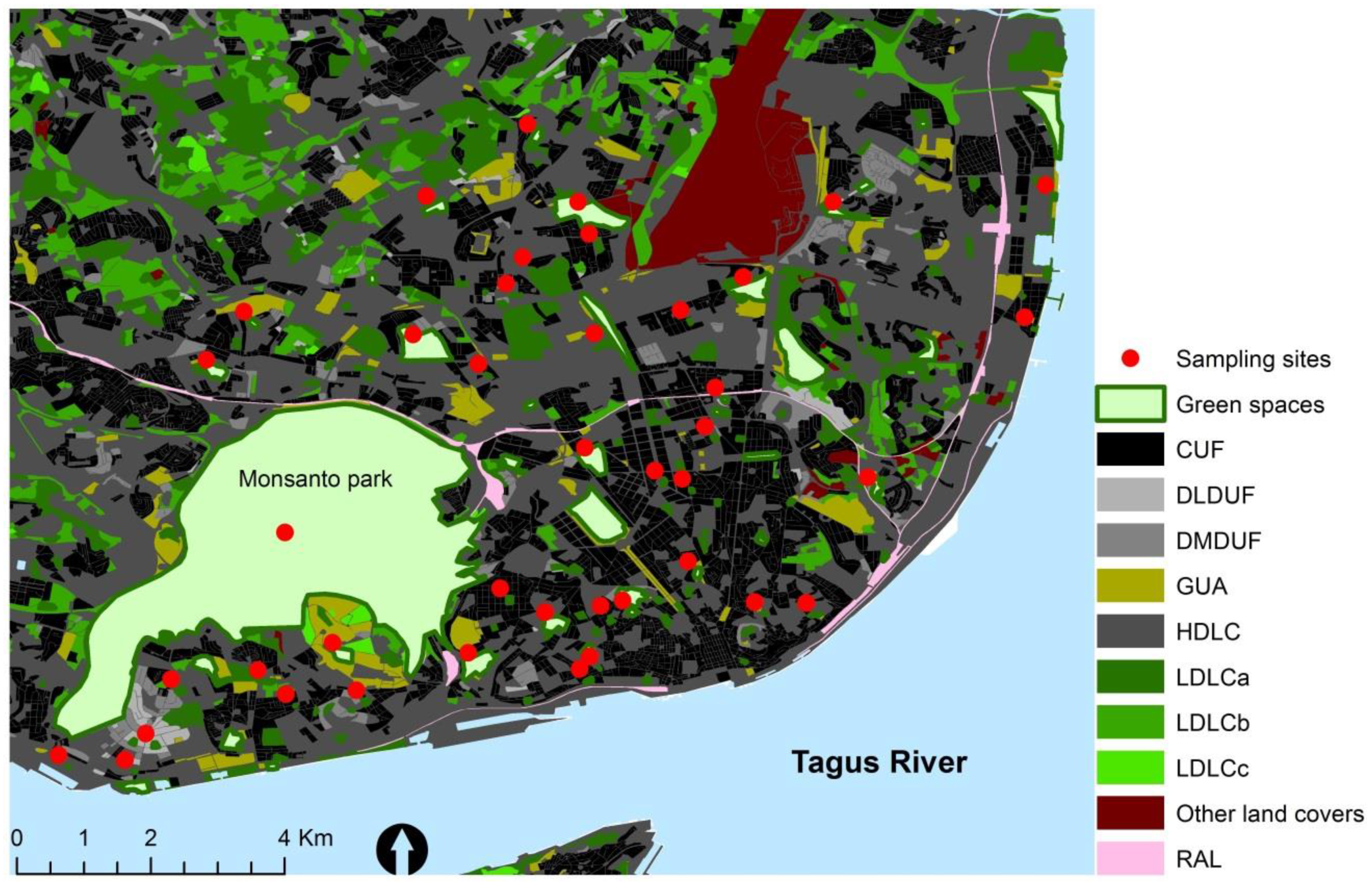
2.2. Lichen Sampling

Macro and micro epiphytic lichens were sampled during March, April, and May of 2015. The four suitable trees closest to the centroid of each sampling site, in each green space, were selected and sampled following the European standard methodology [19]. We opted for using the trees closest to the centroids because they offer the highest potential for disturbance reduction due to the fact that they are the most protected area inside the green space. Although the European methodology [19] recommends using only one species of phorophyte, this was impossible due to the great diversity of phorophytes in Lisbon. We estimate that 60% of phorophytes were Jacaranda mimosifolia D. Don, as this species is one of the most widely spread species in Lisbon green spaces, with the adequate characteristics for this work. Tipuana tipu (Bentham) Kuntze accounted for around 30%, and the rest were from unidentified species, as sampling was conducted during winter, and these remaining phorophytes were all deciduous. To address this limitation, only phorophytes with medium bark roughness were used for sampling.
Sampling was conducted using a grid with 50 cm × 10 cm (divided into five equal squares, 10 cm × 10 cm). The grid was attached at chest height, to the tree trunk facing the four cardinal points, and the frequency of each present species (maximum of 20 and minimum of 1, per tree) was noted. In addition to bark roughness, phorophyte selection also took into account trunk inclination (no more than ten degrees deviation from vertical), diameter at chest height (between 50 cm and 150 cm), and with no visible trunk damage, knots or other obstacles for epiphytic lichens development. All phorophytes’ diameter and coordinates were recorded using a measuring tape and a GPS device, respectively. A magnifying lens was used for in-site species determination. Species that could not be determined in the field were properly collected and stored in envelopes and later identified in a laboratory resorting to a microscope and different identification keys [47,48]. Species nomenclature follows Nimis [36].
Species were classified according to the maximum value of the poleotolerance response trait available in ITALIC [36] (Table 1). Trait classification and species frequencies were combined to calculate the community-weighted mean (CWM) for each functional group, in each green space. The CWM is a trait-based metric representing a measure of functional structure. As this trait is categorical, the CWM here calculated represents the mean proportion of each functional group in the community, weighted by the abundance of species belonging to those groups [49]. CWM was calculated using the “dbFD” function from the FD package [50] of R CRAN software [51].

2.3. Environmental Variables

Three types of variables were calculated for each green space: (1) The area (m2) of each green space; (2) the normalized difference vegetation index (NDVI), both for the green space centroid (NDVIgs) and for a 100 m buffer around each sampling site (NDVIb100), used as a proxy of vegetation density; and (3) the surrounding land cover area around the green space.
Green spaces areas were determined using ArcGIS Desktop 10.6.1 (ESRI). NDVI values refer to May 2015 (to remove the effects of grasslands, after image correction) and were calculated based on a Landsat 8 image (30 meters resolution). NDVIb100 was calculated so we could take into consideration the possible effects of nearby green spaces. NDVI is used as a proxy of vegetation density and green space area. However, that does not necessarily mean that bigger green spaces have higher NDVI values, as the NDVI values are higher or lower depending on the amount of surface covered by green vegetation and not on the area of the green space (e.g., a bigger green space with trees and bare soil will have lower NDVI values than a smaller green space with trees and grass instead of bear soil). Characterization of the land cover surrounding each sampled green space was also made in ArcGIS Desktop 10.6.1 (ESRI) using the information available in the Urban Atlas. Buffers with seven different radii (50 m; 100 m; 200 m; 500 m; 1000 m; 1500 m; 2000 m) were created around each sampling site. Buffers should be interpreted as drawn imaginary circles, with different radius, created with the sole intention to delimit distinct areas around the sampling sites. These buffers were used to identify all land covers surrounding all the sampling sites, at different distances. A total of 25 land covers were listed in, at least, one of the buffers’ distance: Airports; arable land; construction sites; continuous urban fabric (S.L.: >80%); discontinuous dense urban fabric (S.L.: 50–80%); discontinuous medium density urban fabric (S.L.: 30–50%); discontinuous low density urban fabric (S.L.: 10–30%); discontinuous very low density urban fabric (S.L.: <10%); fast transit roads and associated land; forests; green urban areas; herbaceous vegetation associations; industrial, commercial, public, military, and private units; isolated structures; land without current use; mineral extraction and dump sites; open spaces with little or no vegetation; other roads and associated land; pastures; permanent crops; port areas; railways and associated land; sports and leisure facilities; water and wetlands. From the 25 land cover types, five were discarded (airports; construction sites; mineral extraction and dump sites; open spaces with little or no vegetation; and wetlands), as they were not significantly correlated with the CWM nor with the ordination scores, at any buffer distance (Table S1). For the remaining land covers, the best buffer distance was selected. After that, land cover types with the same buffer distance and similar correlation trend (correlation signals) with the first and second axes from the NMS and the CWMs of all three functional groups were grouped. Four groups were created (HDLC; LDLCa; LDLCb; LDLCc).

2.4. Data Analysis

Nonmetric multidimensional scaling (NMS) was performed to identify the main drivers of lichens communities’ changes. This analysis was run in a relativized matrix of species abundances, to avoid biasing results and impairment of comparisons [16]. Bray–Curtis distance was used, and the best NMS solution was chosen from 50 runs (with real data), each starting randomly (500 iterations per run), and evaluated with a Monte Carlo test (250 runs with randomized data). The coefficients of determination (r2) between the original plot distances and distances in the final ordination solution were calculated to assess the community variability represented by the NMS axes [52]. The analysis was run using PC-Ord Software, version 7.03 [53]. Significant functional variables, CWM, were overlaid on the NMS ordination as correlation vectors [52] to confirm species classification. This was done looking at the distance between the position of the CWM of the functional groups and each species, taking also into consideration the position of the environmental variables.
Buffer distance for each land cover was selected individually, as its influence may vary with land cover type. Spearman correlations (to account for possible nonlinearity in the relationships) were performed between NMS scores, the CWM of each functional group, and the environmental variables. Correlations were made in R software [51] and considered significant for p < 0.05. The buffer distance selected for each land cover was the one presenting the higher number of significant correlations with the functional variables [54]. The CWM values of each functional group were then interpolated for the entire city of Lisbon using ordinary kriging. All spatial analysis was done in ArcMap (ESRI, version 10.5).

3. Results

In total, we identified 38 species (Table S2). Of these, two species had an original poleotolerance classification (Table 1) of “natural”, comprising 5.26% of the total, and six species had a poleotolerance classification of “seminatural” (15.79%). The majority of the species (17) were classified as “low disturbance” (44.73%), and 13 species were classified as “high disturbance”, representing the remaining 34.21% species.
The NMS ordination suggested a three-dimensional solution (minimum stress = 10.8%; P = 0.004), as increasing the number of dimensions did not significantly lowered the stress. The first axis accounted for 45.7% of the variance. The second axis explained 32.5% and the third explained 11.0% of the total variance (89.3%). As the third axis explains only a small percentage of the variance, the analysis focuses on the first two axes.

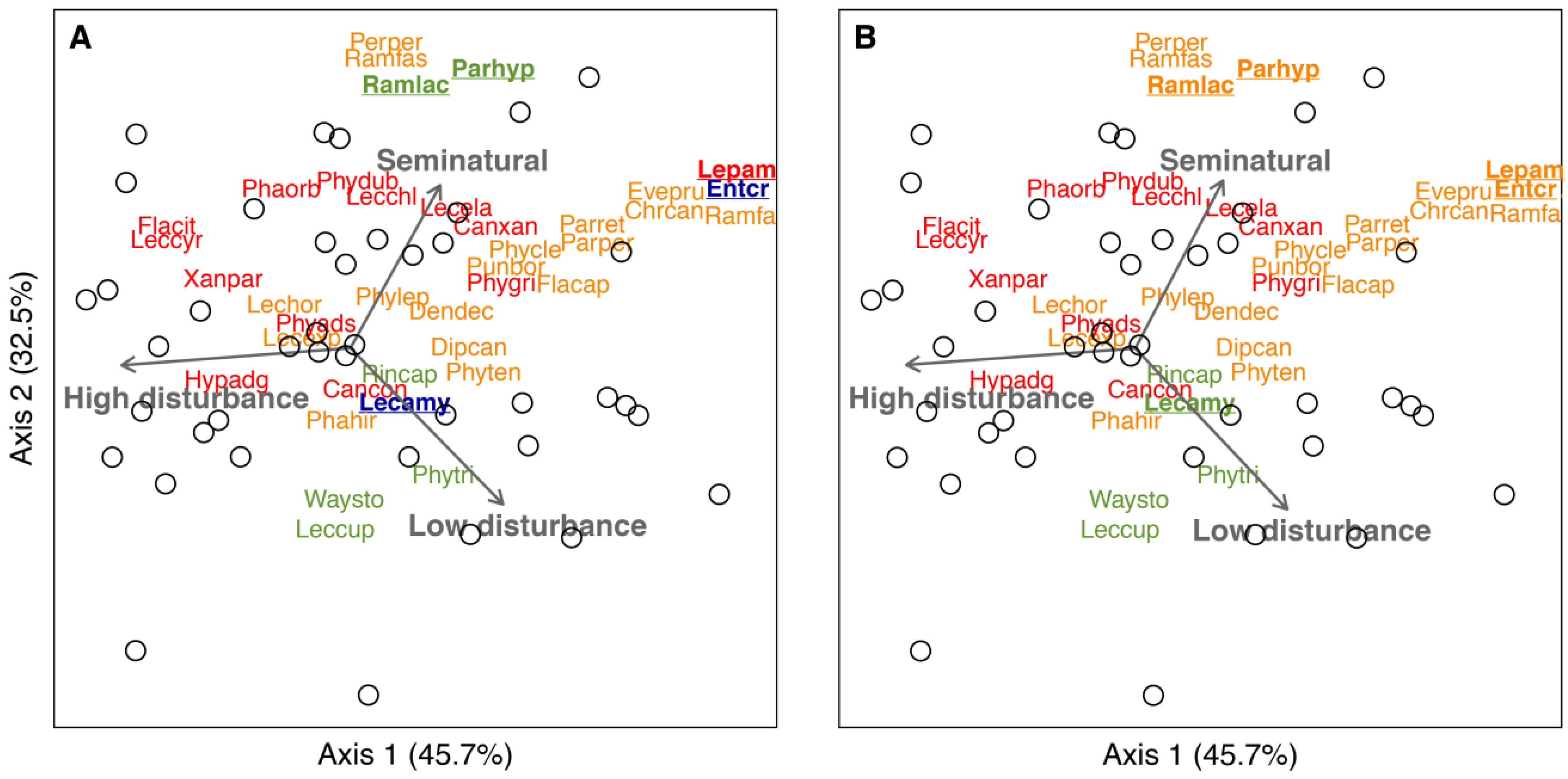
3.1. Confirming Species Classification

The first step was to overlay lichen species ordination scores in the NMS solution, colored by functional group, to understand if the poleotolerance ranking assigned to each species was correct (Figure 2A).
The analysis of the ordination revealed five clearly misclassified species, i.e., located in the opposite side of the gradient where the CWM of that functional group is higher. Enterographa crassa (DC.) Fée was classified as natural and was reclassified to low disturbance. Lecanographa amylacea (Pers.) Egea and Torrente from natural to seminatural. Lepra amara (Ach.) Hafellner from high disturbance to low disturbance. Finally, Parmotrema hypoleucinum (J. Steiner) Hale and Ramalina lacera (With.) J.R. Laundon from seminatural to low disturbance. The CWM was recalculated using this new classification (Figure 2B).

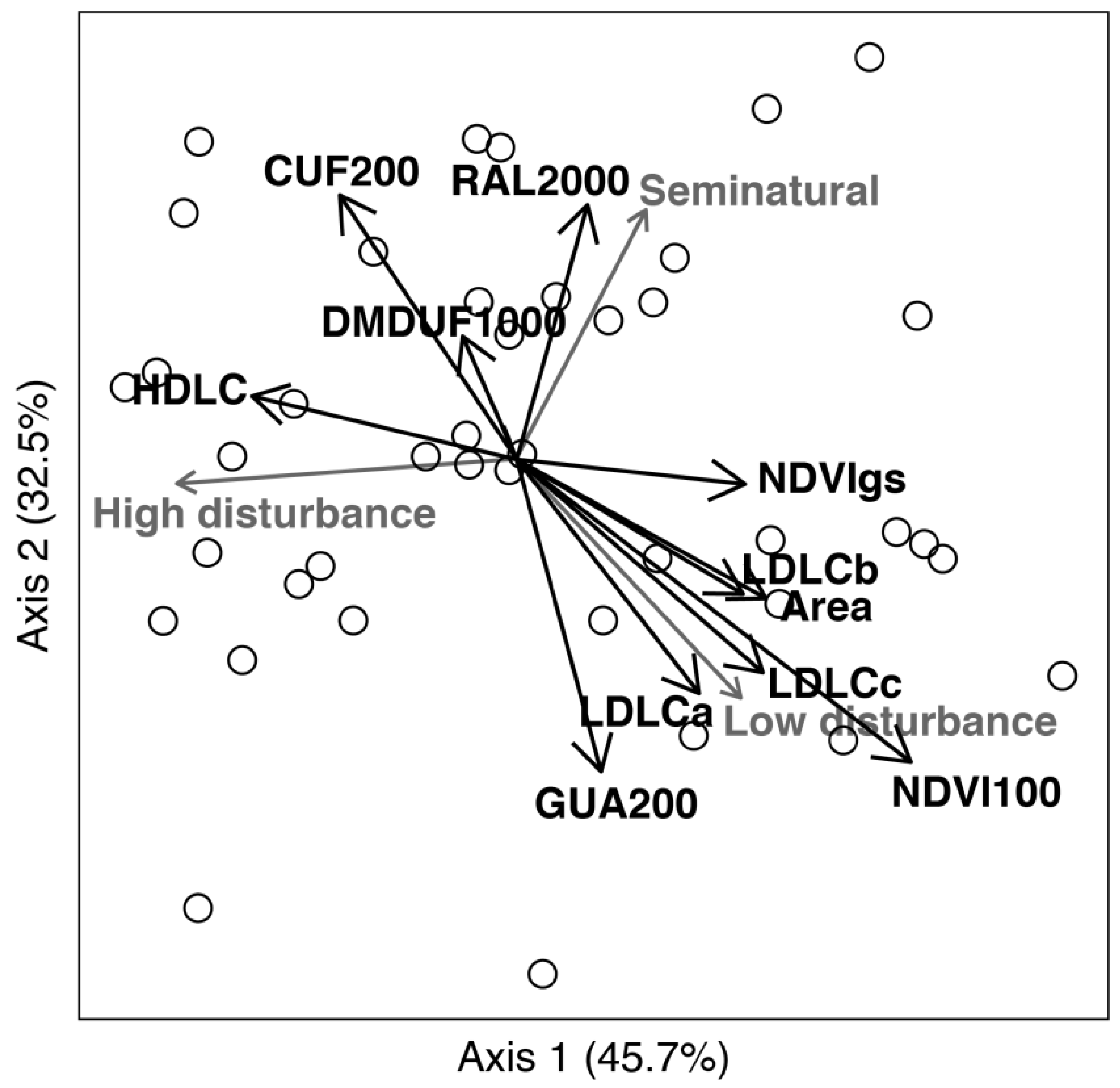
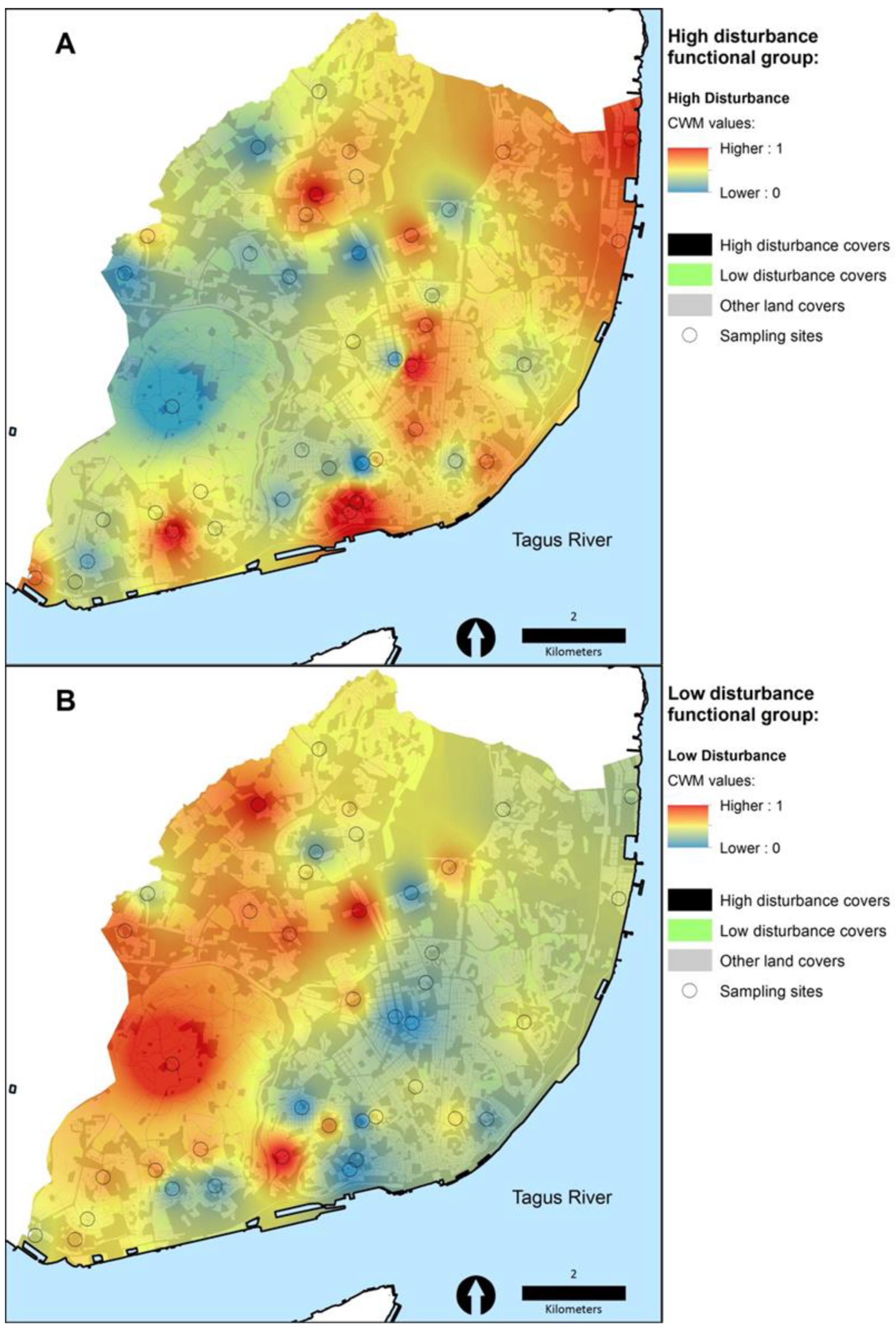
3.2. The Poleotolerance Response Trait as an Indicator of Urban Disturbance

Ordination scores and the CWM of all functional groups were correlated with the environmental variables to determine the size of the buffer to use for each land cover (Table S1). As previously stated, from the 25 land cover types, five were immediately discarded. Remaining land cover types were grouped based on their buffer distances and correlation trends. From there, four groups were created. The first group was the HDLC (high disturbance land covers) comprising five land covers (all at a 500 m buffer) associated with high human disturbance (discontinuous dense urban fabric; industrial, commercial, public, military, and private units; port areas; other roads and associated land; water). The remaining three groups comprise land covers associated with low human disturbance, the low disturbance land covers (LDLC), with three different buffer distances: LDLCa, LDLCb, and LDLCc, with 1000, 1500, and 2000 meter buffers, respectively. LDLCa comprises the arable land, herbaceous vegetation associations, and sports and leisure facilities land covers. LDLCb comprises the fast transit roads and associated land, land without current use, pastures, and permanent crops. LDLCc comprises the discontinuous very low-density urban fabric, forests, and isolated structures.
Correlations between the CWM and the axes scores and the best buffers are shown in Table 2.
The environmental variables that were significantly correlated with ordination axes scores were overlaid in the solution as correlational vectors (Figure 2B). Correlations between site ordination scores and environmental variables suggest that the first axis (Table 2) is reflecting a gradient of anthropic disturbance. On the most disturbed side of the gradient, we have land covers associated with high anthropic presence and disturbance: Continuous urban fabric (200 m buffer) and land covers from the HDLC group. On the less disturbed side, we have land covers associated with seminatural areas comprising the LDLCa, LDLCb and LDLCc land-cover groups. The remaining land covers are not significantly correlated with the first axis. In addition, both NDVI values (NDVIgs and NDVIb100) and the area of the green spaces were also associated with the less disturbed side of the gradient. The second axis also revealed a gradient of disturbance, though less evident than the first: One side is associated with the discontinuous medium density urban fabric (1000 m buffer) and railways and associated land (2000 m buffer) land covers (both associated to higher disturbance levels); the other one with green urban areas (200 m buffer) land cover (associated to lower disturbance levels), the area of the green spaces, and the NDVIb100. The remaining land covers were not significantly correlated with this axis. For more detailed data, see Table S3).
To understand if the poleotolerance response trait was, in fact, mediating lichen species’ response to this disturbance gradient, the CWM of poleotolerance functional groups were also overlaid in the solution as vectors (Figure 3). The high disturbance functional group was associated with the most disturbed side of the gradient. The significant correlations between the high disturbance CWM values with several environmental variables corroborate this result (Table 2). The low disturbance functional group was associated with the opposite side of the disturbance gradient (Figure 2B). Again, the low disturbance result was corroborated by the correlations with the environmental variables (Table 2). Lastly, the seminatural functional group was also associated to the low disturbance side of the gradient, though to a lesser extent than the two other functional groups (Table 2). This functional group was positioned in the middle of the first axis disturbance gradient but clearly separated by the other two functional groups in the second axis, being positioned on the higher disturbance side of the second axis gradient. However, this functional group was only significantly correlated with the discontinuous medium density urban fabric (1000 m buffer) and the LDLCb land cover group.
The CWMs values of each functional group in the 41 sampling sites were interpolated for the entire city of Lisbon to have a spatial distribution of anthropic disturbance levels indicated by the poleotolerance trait. In general, spatial patterns of high disturbance and low disturbance functional groups indicate that the most disturbed areas in Lisbon (orange and red areas in Figure 4A; blue and green in Figure 4B) are located closer to the airport and the city center, while low anthropic areas can be found close to Monsanto and further away from the city center (Figure 4A,B). The spatial pattern of the seminatural functional group shows no clear pattern in Lisbon, being diffuse throughout the south and southeast part of the city (Figure 4C).

4. Discussion

This study presents a novelty regarding the application of the poleotolerance response trait as an ecological indicator of human disturbance in urban environments. This trait was able to differentiate highly disturbed green spaces from those with lower levels of anthropic disturbance. The two functional groups with higher tolerance to greater disturbed areas showed to be efficient in this task. On the other hand, the seminatural functional group also indicated low levels of disturbance but failed to indicate the green spaces more similar to seminatural habitats.
We were able to identify five misclassified species in the poleotolerance response trait (Enterographa crassa, Lecanographa amylacea, Lepra amara, Parmotrema hypoleucinum, and Ramalina lacera). These results confirm that lichens distribution is a result of multiple interacting biotic and abiotic factors that may result in different ecological behaviors regarding anthropic disturbance. The fact that this trait classification was elaborated based only on studies conducted in Italy may potentially increase the probability of misclassifying species from regions with contrasting biotic and abiotic factors (climate, for example). Such a situation has already been reported by Pinho et al. [55] for the trait classification regarding epiphytic lichens tolerance to nitrogen pollution. Other authors also found contrasting classifications in different regions from the United States of America, something they attributed to climatic differences [56].
According to Nimis [36], the poleotolerance response trait classification should reflect lichens’ ability to occur in areas with different levels of human disturbance. The disturbance gradient along Lisbon green spaces has been recently attributed to a strong background pollution gradient [14]. Our results showed that the functional groups with high and low tolerance to disturbance were able to successfully identify such a disturbance gradient. We saw that green spaces with bigger areas, higher NDVI values, and surrounded by low disturbance land covers (LDLCa/b/c) were those with lower anthropic disturbance (high CWM of low disturbance functional group and low CWM of the high disturbance functional group). Only one study has previously used this trait in an urban context [23]. The authors saw that in Rome, low and high disturbance functional groups accounted for 51% of total species (38% and 13%, respectively), but no discussion of the relationship of its patterns and urban disturbance was made. In Lisbon, we found that 87% of the lichen species were classified in these two groups (55% and 32%, respectively), a number significantly higher than that found for Rome. Our results showed that spatially, the higher anthropic disturbance areas are located close to the airport and the city center (Figure 4A,B), coinciding with those previously highlighted as with lower air quality [14]. Conversely, the spatial distribution of these functional groups showed that low disturbance green spaces are located in the area of Lisbon with the largest green space, Monsanto (Figure 4A,B), also matching the area previously pointed as with best air quality [14]. Thus, our results show that high and low disturbance functional groups have not only the potential to be applied in urban environments, but they can also be a useful tool to spatially signal the disturbance areas in a city, which can be used as a tool for better management practices in cities.
Similarly to the low disturbance functional group, the seminatural functional group also indicated low levels of disturbance, although without a clear spatial pattern. This could be due to the fact that only a very small proportion of the sampled lichen species were representative of this functional group, and it was thus difficult to produce robust results with it. Only two species belonged initially to the natural functional group but were reclassified and merged with the seminatural. As a result, after the reclassification, there were five species classified as seminatural out of the 38 total (13.16%). The low representativeness of natural and seminatural species may be a clue pointing to the lack of truly natural habitats. We expected that the seminatural functional group would be significantly positively correlated with the area of the green spaces, as bigger areas would work as a stopper for a surrounding disturbance. However, that did not happen. We sampled five green spaces with areas equal or higher than 10 ha, expecting these to represent seminatural areas (Monsanto—1000 ha; Quinta das Conchas—23 ha; Parque Bensaúde—22 ha; Parque José Gomes Ferreira—10 ha, and Tapada das Necessidades—10 ha). Monsanto is by far the largest green space in Lisbon, with dense vegetation throughout the whole area. Quinta das Conchas and Parque José Gomes Ferreira are both close to the airport and to one of the busiest roads in Lisbon and both have sparse vegetation. Parque Bensaúde also has sparse vegetation, and it is located right next to another high traffic road (Avenida Lusíada). Lastly, Tapada das Necessidades is composed of dense vegetation and sits close to the port area and the river Tagus. Thus, though they are big enough to buffer disturbance effects, the fact that they have low-density vegetation and/or they are located next to high disturbance sites (like the airport or major roads) may somewhat prevent them from being true seminatural areas. This translates into a lack of robustness of results regarding this functional group. We should however note that Reference [23] concluded that the high percentage (~50%) of seminatural and natural poleotolerance classified epiphytic lichens, in Rome, was due to a successful city environmental planning. Thus, it is possible that other cities may have the necessary environmental characteristics to house this type of lichens species. The fact that, in our work, natural and seminatural functional groups had a low representation may be seen as a limitation for the application of this trait in highly disturbed cities. In fact, in Lisbon, it is very difficult, if not impossible, to identify and sample green spaces that fall into the description provided by Nimis et al. [36], characterizing the habitat for these two functional groups (Table 1). Thus, we recommend that future works should take this factor into consideration when preparing the sample design, so that in cities like Lisbon, with high disturbance levels, sampling sites are characterized as natural or seminatural areas, even if located in the outskirts of the urban perimeter are included.
In this work, we intentionally focused on a single trait, poleotolerance, with the purpose of understanding if this trait could be useful as an indicator of anthropic disturbances in an urban context. Our results showed a shift in lichen communities from low tolerance species to high tolerance species as we moved to more disturbed areas. A recent work [14] using the same methodology in the same study area explored three other, different traits, growth form, eutrophication tolerance, and humidity requirements, and did not observe any shifts in lichen communities mediated by these three traits. This is an indication that in urban environments, such as this encountered in Lisbon, the use of the poleotolerance trait may be more advantageous than using other, more commonly used traits, giving a clearer indication about the disturbance gradient. Humidity requirements, growth form, and eutrophication tolerance are frequently used to indicate disturbance related to the urban heat island effect (microclimatic variations) and nitrogen pollution. The fact that poleotolerance trait performed better here is the advantage of using it when we are not able to clearly disentangle those two environmental drivers, highlighting its potential as an integrated indicator of overall anthropic disturbance in urban settlements. The presence of pruina or secondary metabolites also showed promising results in South American cities as indicators of the effects of disturbances associated to urban environments [28,57]. In our work, we did not test these traits. The poleotolerance is, for now, restricted to Southern European cities that share some of the lichen flora of Italy. Pruina or secondary metabolites have the advantage of being independent of this classification, having therefore more potential to be applied outside Europe, so future works should try to explore it in Europe, to understand if they also have the potential to be used here. We also suggest, for future works focusing on this trait, that, if possible, datasets of population densities and distributions should be used, as these types of data can be a very suitable proxy for human disturbance levels inside the studied areas.

5. Conclusions

We conclude that the poleotolerance response trait can be used to distinguish areas with different anthropic disturbance levels in regions of Europe apart from Italy. Both the high disturbance and the low disturbance functional groups enabled us to identify a gradient of anthropic disturbance. However, the seminatural functional group did not, and that is probably related to the low number of species belonging to this functional group, possibly due to the lack of truly natural green spaces in our study area. Further studies should try to fully elucidate if this is a trait limitation or a sampling design issue. Because this is an integrative trait, it has the potential to be used even when we do not know the underlying environmental factors driving changes, signaling disturbed areas that should deserve further attention in future studies to individually assess the drivers of change, a very important tool under an urban management perspective.
To sum up, even with the limitations that may arise, mostly due to the fact that species classification may not be present in the Italian database, our work showed that the poleotolerance response trait has potential to be used in urban environments in other Southern European cities. Future studies should consider enlarging the trait database for Europe, allowing its use for wider geographical regions.

Supplementary Materials

The following are available online at https://www.mdpi.com/1424-2818/11/4/55/s1, Table S1: Spearman correlations between lichen community ordination axes (NMS1, NMS2, and NMS3), lichens CWM (high disturbance, low disturbance, and seminatural) and the 25 land covers, Table S2: Epiphytic lichen species collected and identified, and Poleotolerance classification of each species prior and after reclassification, Table S3: Spearman correlation coefficients between lichen community ordination axes (NMS1, NMS2, and NMS3), lichens CWM (high disturbance, low disturbance, and seminatural) and the environmental variables, Table S4: Land covers groups and respective land covers within each group, based on the classifications from Figure 4.

Author Contributions

Conceptualization, P.P., C.B. and P.M.; Formal analysis, B.R. and P.M.; Funding acquisition, P.P. and C.B.; Methodology, P.P., J.V., C.B. and P.M.; Writing—original draft, B.R., P.P., C.B. and P.M.

Funding

Pedro Pinho acknowledges H2020/FCT BiodivERsA 32015104 (BioVeins) and H2020/TWINN 692331 (NitroPortugal) for funding. Paula Matos acknowledges FCT PTDC/AAG-GLO/0045/2014 (ChangeTracker) for funding.

Conflicts of Interest

The authors declare no conflict of interest.

References

  1. Roser, M.; Ortiz-Ospina, E. World Population Growth. 2019. Available online: https://ourworldindata.org/world-population-growth:OurWorldInData.org (accessed on 19 December 2018).
  2. Lutz, W.; Sanderson, W.C.; Scherbov, S. Probabilistic World Population Projections Based on ExpertOpinion; IIASA—International Institute for Applied Systems Analysis: Laxenburg, Austria, 1996. [Google Scholar]
  3. Agency, E.E. Increasing Environmental Pollution (GMT 10); European Union: Brussels, Belgium, 2015; pp. 1–5. [Google Scholar]
  4. Rosenzweig, C.; Iglesias, A.; Yang, X.; Epstein, P.R.; Chivian, E. Climate change and extreme weather events; implications for food production, plant diseases, and pests. Glob. Chang. Hum. Health 2001, 2, 90–104. [Google Scholar] [CrossRef]
  5. Achard, F.; Eva, H.D.; Stibig, H.-J.; Mayaux, P.; Gallego, J.; Richards, T.; Malingreau, J.-P. Determination of deforestation rates of the world’s humid tropical forests. Science 2002, 297, 999–1002. [Google Scholar] [CrossRef] [PubMed]
  6. DeFries, R.S.; Rudel, T.; Uriarte, M.; Hansen, M. Deforestation driven by urban population growth and agricultural trade in the twenty-first century. Nat. Geosci. 2010, 3, 178. [Google Scholar] [CrossRef]
  7. Boyd, B. Urbanization and the Mass Movement of People to Cities. Available online: https://graylinegroup.com/urbanization-catalyst-overview/ (accessed on 28 December 2018).
  8. United Nations, Department of Economic and Social Affairs, Population Division. World Urbanization Prospects: The 2014 Revision-Highlights; UN (ST/ESA/SER.A/352): New York, NY, USA, 2014. [Google Scholar]
  9. Niemi, G.J.; McDonald, M.E. Application of ecological indicators. Annu. Rev. Ecol. Evol. Syst. 2004, 35, 89–111. [Google Scholar] [CrossRef]
  10. Ludwig, J.A.; Tongway, D.J.; Bastin, G.N.; James, C.D. Monitoring ecological indicators of rangeland functional integrity and their relation to biodiversity at local to regional scales. Austral Ecol. 2004, 29, 108–120. [Google Scholar] [CrossRef]
  11. Marinari, S.; Mancinelli, R.; Campiglia, E.; Grego, S. Chemical and biological indicators of soil quality in organic and conventional farming systems in Central Italy. Ecol. Indic. 2006, 6, 701–711. [Google Scholar] [CrossRef]
  12. McCune, B. Lichen communities as indicators of forest health. Bryologist 2000, 103, 353–356. [Google Scholar] [CrossRef]
  13. Nilsson, S.G.; Arup, U.; Baranowski, R.; Ekman, S. Tree-dependent lichens and beetles as indicators in conservation forests. Conserv. Biol. 1995, 9, 1208–1215. [Google Scholar] [CrossRef]
  14. Matos, P.; Vieira, J.; Rocha, B.; Branquinho, C.; Pinho, P. Modeling the provision of air-quality regulation ecosystem service provided by urban green spaces using lichens as ecological indicators. Sci. Total Environ. 2019, 665, 521–530. [Google Scholar] [CrossRef] [PubMed]
  15. Vieira, J.; Matos, P.; Mexia, T.; Silva, P.; Lopes, N.; Freitas, C.; Correia, O.; Santos-Reis, M.; Branquinho, C.; Pinho, P. Green spaces are not all the same for the provision of air purification and climate regulation services: The case of urban parks. Environ. Res. 2018, 160, 306–313. [Google Scholar] [CrossRef]
  16. Matos, P.; Pinho, P.; Aragon, G.; Martínez, I.; Nunes, A.; Soares, A.M.; Branquinho, C. Lichen traits responding to aridity. J. Ecol. 2015, 103, 451–458. [Google Scholar] [CrossRef] [Green Version]
  17. Aptroot, A.; Van Herk, C. Further evidence of the effects of global warming on lichens, particularly those with Trentepohlia phycobionts. Environ. Pollut. 2007, 146, 293–298. [Google Scholar] [CrossRef] [PubMed]
  18. Ohmura, Y.; Seaward, M.R. Is Glyphis cicatricosa an indicator for ‘global warming’or an ‘urban heat island’effect in Japan? Lichenologist 2017, 49, 291–296. [Google Scholar] [CrossRef]
  19. Asta, J.; Erhardt, W.; Ferretti, M.; Fornasier, F.; Kirschbaum, U.; Nimis, P.; Purvis, O.; Pirintsos, S.; Scheidegger, C.; Van Haluwyn, C. Mapping lichen diversity as an indicator of environmental quality. In Monitoring with Lichens—Monitoring Lichens; Springer: Berlin/Heidelberg, Germany, 2002; pp. 273–279. [Google Scholar]
  20. Smith, W.B. Forest inventory and analysis: A national inventory and monitoring program. Environ. Pollut. 2002, 116, S233–S242. [Google Scholar] [CrossRef]
  21. Llop, E.; Pinho, P.; Matos, P.; Pereira, M.J.; Branquinho, C. The use of lichen functional groups as indicators of air quality in a Mediterranean urban environment. Ecol. Indic. 2012, 13, 215–221. [Google Scholar] [CrossRef]
  22. Saiki, M.; Fuga, A.; Alves, E.; Vasconcellos, M.; Marcelli, M. Biomonitoring of the atmospheric pollution using lichens in the metropolitan area of São Paulo city, Brazil. J. Radioanal. Nucl. Chem. 2006, 271, 213–219. [Google Scholar] [CrossRef]
  23. Munzi, S.; Ravera, S.; Caneva, G. Epiphytic lichens as indicators of environmental quality in Rome. Environ. Pollut. 2007, 146, 350–358. [Google Scholar] [CrossRef] [PubMed]
  24. Munzi, S.; Correia, O.; Silva, P.; Lopes, N.; Freitas, C.; Branquinho, C.; Pinho, P. Lichens as ecological indicators in urban areas: Beyond the effects of pollutants. J. Appl. Ecol. 2014, 51, 1750–1757. [Google Scholar] [CrossRef]
  25. Branquinho, C.; Serrano, H.C.; Nunes, A.; Pinho, P.; Matos, P. From Assessing to Conserving Biodiversity. In History, Philosophy and Theory of the Life Sciences, 1st ed.; Casetta, E., Silva, J.M.D., Vecchi, D., Eds.; Springer International Publishing: Berlin/Heidelberg, Germany, 2019; p. 290. [Google Scholar]
  26. Dıaz, S.; Cabido, M. Vive la difference: Plant functional diversity matters to ecosystem processes. Trends Ecol. Evol. 2001, 16, 646–655. [Google Scholar] [CrossRef]
  27. Mouillot, D.; Villéger, S.; Parravicini, V.; Kulbicki, M.; Arias-González, J.E.; Bender, M.; Chabanet, P.; Floeter, S.R.; Friedlander, A.; Vigliola, L. Functional over-redundancy and high functional vulnerability in global fish faunas on tropical reefs. Proc. Natl. Acad. Sci. USA 2014, 111, 13757–13762. [Google Scholar] [CrossRef] [Green Version]
  28. Koch, N.M.; Matos, P.; Branquinho, C.; Pinho, P.; Lucheta, F.; de Azevedo Martins, S.M.; Vargas, V.M.F. Selecting lichen functional traits as ecological indicators of the effects of urban environment. Sci. Total Environ. 2019, 654, 705–713. [Google Scholar] [CrossRef]
  29. Varela, Z.; López-Sánchez, G.; Yáñez, M.; Pérez, C.; Fernández, J.; Matos, P.; Branquinho, C.; Aboal, J. Changes in epiphytic lichen diversity are associated with air particulate matter levels: The case study of urban areas in Chile. Ecol. Indic. 2018, 91, 307–314. [Google Scholar] [CrossRef]
  30. Barkman, J.J. Phytosociology and Ecology of Cryptogamic Epiphytes; Van Gorcum, University of Michigan: Ann Arbor, MI, USA, 1958. [Google Scholar]
  31. DeSLOOVER, J. Mapping on atmospheric pollution on the basis of lichen sensitivity. Proc. Symposium Recent Adv. Trop. Ecol. 1968, 1, 42–56. [Google Scholar]
  32. Trass, H. Lichen sensitivity to the air pollution and index of poleotolerance (IP). Folia Cryptog Est. 1973, 3, 19–22. [Google Scholar]
  33. Nimis, P.L. The Epiphytic Lichen Vegetation of the Trieste Province (North Eastern Italy); EUT Edizioni Università di Trieste: Triste, Italy, 1982. [Google Scholar]
  34. Nimis, P. Urban Lichen Studies in Italy. II: The town of Udine. Gortania 1986, 7, 147–172. [Google Scholar]
  35. Nimis, P. Urban lichen studies in Italy. III: The city of Rome. Braun-Blanquetia 1989, 2, 223–238. [Google Scholar]
  36. Nimis, P.L. The Lichens of Italy. A Second Annotated Catalogue; EUT Edizioni Università di Trieste: Triste, Italy, 2016. [Google Scholar]
  37. Degtjarenko, P.; Matos, P.; Marmor, L.; Branquinho, C.; Randlane, T. Functional traits of epiphytic lichens respond to alkaline dust pollution. Fungal Ecol. 2018, 36, 81–88. [Google Scholar] [CrossRef]
  38. Nimis, P.L.; Martellos, S.; Spitale, D.; Nascimbene, J. Exploring patterns of commonness and rarity in lichens: A case study from Italy (Southern Europe). Lichenologist 2018, 50, 385–396. [Google Scholar] [CrossRef]
  39. Gilbert, O. Further studies on the effect of sulphur dioxide on lichens and bryophytes. New Phytol. 1970, 69, 605–627. [Google Scholar] [CrossRef]
  40. Branquinho, C.; Matos, P.; Pinho, P. Lichens as ecological indicators to track atmospheric changes: Future challenges. In Indicators and Surrogates of Biodiversity and Environmental Change; CSIRO Publishing: Melbourne, Australian; CRC Press: London, UK, 2015; pp. 77–87. [Google Scholar]
  41. Nowak, D.J.; Jovan, S.; Branquinho, C.; Augusto, S.; Ribeiro, M.C.; Kretsch, C.E. Biodiversity, air quality and human health. In Connecting Global Priorities: Biodiversity and Human Health: A State of Knowledge Review; World Health Organization: Geneva, Switzerland, 2015. [Google Scholar]
  42. INE. Censos 2011 Resultados Definitivos-Portugal; Instituto Nacional de Estatística, IP: Lisboa, Portugal, 2012. [Google Scholar]
  43. Kottek, M.; Grieser, J.; Beck, C.; Rudolf, B.; Rubel, F. World map of the Köppen-Geiger climate classification updated. Meteorol. Z. 2006, 15, 259–263. [Google Scholar] [CrossRef]
  44. PORDATA. Available online: https://www.pordata.pt/Portugal (accessed on 15 January 2019).
  45. Económico, O.J. Todos os dias entram 370 mil carros em Lisboa. O Jornal Económico. Available online: https://jornaleconomico.sapo.pt/noticias/os-dias-entram-lisboa-370-mil-carros-84046 (accessed on 6 April 2019).
  46. EEA. Copernicus Land Monitoring Service—Urban Atlas. 2018. Available online: www.eea.europa.eu/data-and-maps/data/copernicus-land-monitoring-service-urban-atlas (accessed on 10 January 2015).
  47. Martellos, S. Multi-authored interactive identification keys: The FRIDA (FRiendly IDentificAtion) package. Taxon 2010, 59, 922–929. [Google Scholar] [CrossRef]
  48. Smith, C.W.; Aptroot, A.; Coppins, B.J.; Fletcher, A.; Gilbert, O.L.; James, P.W.; Wolseley, P.A. The Lichens of Great Britain and Ireland; British Lichen Society: London, UK, 2009. [Google Scholar]
  49. Lavorel, S.; Grigulis, K.; McIntyre, S.; Williams, N.S.; Garden, D.; Dorrough, J.; Berman, S.; Quétier, F.; Thébault, A.; Bonis, A. Assessing functional diversity in the field–methodology matters! Funct. Ecol. 2008, 22, 134–147. [Google Scholar] [CrossRef]
  50. Laliberté, E.; Legendre, P.; Shipley, B. FD: Measuring Functional Diversity from Multiple Traits, and Other Tools for Functional Ecology, R package version 1.0-12; R Foundation for Statistical Computing: Vienna, Austria, 2014. [Google Scholar]
  51. R Core Team. R: A Language and Environment for Statistical Computing; R Core Team: Vienna, Austria, 2013. [Google Scholar]
  52. McCune, B.; Grace, J.B.; Urban, D.L. Analysis of Ecological Communities; MjM Software Design: Gleneden Beach, OR, USA, 2002; Volume 28. [Google Scholar]
  53. McCune, B.; Mefford, M. PC-ORD: Multivariate Analysis of Ecological Data; Version 4 for Windows; [User’s Guide]; MjM Software Design: Gleneden Beach, OR, USA, 1999. [Google Scholar]
  54. Pinho, P.; Augusto, S.; Maguas, C.; Pereira, M.; Soares, A.; Branquinho, C. Impact of neighbourhood land-cover in epiphytic lichen diversity: Analysis of multiple factors working at different spatial scales. Environ. Pollut. 2008, 151, 414–422. [Google Scholar] [CrossRef] [PubMed]
  55. Pinho, P.; Dias, T.; Cruz, C.; Sim Tang, Y.; Sutton, M.A.; Martins-Loução, M.A.; Máguas, C.; Branquinho, C. Using lichen functional diversity to assess the effects of atmospheric ammonia in Mediterranean woodlands. J. Appl. Ecol. 2011, 48, 1107–1116. [Google Scholar] [CrossRef] [Green Version]
  56. Root, H.T.; Geiser, L.H.; Jovan, S.; Neitlich, P. Epiphytic macrolichen indication of air quality and climate in interior forested mountains of the Pacific Northwest, USA. Ecol. Indic. 2015, 53, 95–105. [Google Scholar] [CrossRef]
  57. Valencia-Islas, N.; Zambrano, A.; Rojas, J. Ozone reactivity and free radical scavenging behavior of phenolic secondary metabolites in lichens exposed to chronic oxidant air pollution from Mexico City. J. Chem. Ecol. 2007, 33, 1619–1634. [Google Scholar] [CrossRef] [PubMed]
Figure 1. Study area showing the distribution of the sampling sites (red circles; n = 41) within the green spaces and the city’s land covers (adapted from Urban Atlas 2012). Green Spaces; CUF—Continuous urban fabric (S.L.: >80%); DLDUF—Discontinuous low density urban fabric (S.L.: 10–30%); DMDUF—Discontinuous medium density urban fabric (S.L.: 30–50%); GUA—Green urban areas; HDLC—High disturbance land covers; LDCLa—Low disturbance land covers (1000 m buffer); LDCLb—Low disturbance land covers (1500 m buffer); LDCLc—Low disturbance land covers (2000 m buffer); Other land covers and RAL—Railways and associated land. Monsato Forest Park is the biggest green space present in our study area.
Diversity 11 00055 g001
Figure 2. Nonmetric multidimensional scaling (NMS) ordination plot of Lisbon urban green spaces (hollow circles; n = 41) according to lichen species composition with overlaying vectors representing the community weighted mean (CWM) of the functional groups belonging to the poleotolerance trait. (A) Shows species colored with the original classification (misclassified species underlined) and the corresponding CWM vectors. (B) Shows species colored after classification correction (reclassified species underlined) and the CWM functional group vectors recalculated after this correction. Each color represents one of the lichen functional groups (high disturbance—red; low disturbance—orange; seminatural—green; natural—blue). The first two axes explain, respectively, 45.7% and 32.5% of the variance. Only significant variables are shown to prevent overcrowding. See species code names in Annex I.
Diversity 11 00055 g002
Figure 3. NMS ordination plot showing the ordination of sampling sites (hollow circles; n = 41) after correction of species classification. Black vectors represent the environmental variables and grey vectors represent the CWM of the three functional groups (high disturbance, low disturbance, and seminatural). The first two axes explain, respectively, 45.7% and 32.5% of the variance. Environmental variables: Area is the area of each green space; NDVIgs is the normalized difference vegetation index (NDVI) value for the green space centroid; NDVI100 is the NDVI value for a 100 m buffer around each green space centroid; CUF—Continuous urban fabric (S.L.: >80%); DMDUF—Discontinuous medium density urban fabric (S.L.: 30–50%); GUA—Green urban areas; RAL—Railways and associated land; HDLC—High disturbed land covers; LDCLa—Low disturbed land covers (1000 m buffer); LDCLb—Low disturbed land covers (1500 m buffer); LDCLc—Low disturbed land covers (2000 m buffer). Only significant variables are shown to prevent overcrowding. See species code names in Annex I.
Diversity 11 00055 g003
Figure 4. Spatial interpolation of the community weighted mean (CWM) values of the three functional groups of the poleotolerance trait in the 41 sampling sites in Lisbon: (A) represents the pattern of high disturbance functional group CWM; (B) the low disturbance functional group CWM. Areas colored in a gradient from blue to red signal represent increasing values of CWM. (C) The CWMs of the seminatural functional group. Areas colored in a gradient from blue to red signal represent increasing values of CWM. Empty circles indicate the sampling sites. Land cover details can be seen in Table S4.
Diversity 11 00055 g004aDiversity 11 00055 g004b
Table 1. Description of each of the four functional groups of the poleotolerance response trait. Description follows as in Nimis [36].
Functional GroupDescription
NaturalSpecies which exclusively occur on old trees in ancient, undisturbed forests.
SeminaturalSpecies occurring in natural or seminatural habitats
Low disturbanceSpecies occurring in moderately disturbed areas
High disturbanceSpecies occurring in heavily disturbed areas
Table 2. Spearman correlation coefficients between lichen community ordination axes (NMS1, NMS2, and NMS3), lichens CWM (high disturbance, low disturbance, and seminatural) and the environmental variables. Significance level is indicated by the asterisk: * = p < 0.05; ** = p < 0.01; *** = p < 0.001. Environmental variables: Area is the area of each green space; NDVIgs is the NDVI value for the green space centroid; NDVIb100 is the NDVI value for a 100 m buffer around each green space centroid; CUF—Continuous urban fabric (S.L.: >80%); DLDUF—Discontinuous low density urban fabric (S.L.: 10–30%); DMDUF—Discontinuous medium density urban fabric (S.L.: 30–50%); GUA—Green urban areas; RAL—Railways and associated land; HDLC—High disturbed land covers; LDCLa—Low disturbed land covers (1000 m buffer); LDCLb—Low disturbed land covers (1500 m buffer); LDCLc—Low disturbed land covers (2000 m buffer).
AreaNDVIgsNDVIb100CUF200DLDUF100DMDUF1000GUA200RAL2000HDLCLDLCaLDLCbLDLCc
NMS10.54 ***0.34 *0.65 ***−0.33 *−0.010.010.120.12−0.35 *0.34 *0.49 **0.34 *
NMS20.40 *0.010.39 *−0.27−0.01−0.40 * 0.45 ** −0.36 * −0.130.30.150.22
NMS30.140.0600.06−0.36 * −0.02−0.020.060.05−0.13−0.05−0.01
CWM High disturbance−0.41 **−0.34 *−0.57 ***0.3−0.15−0.18−0.01−0.090.35 *−0.32 *−0.43 **−0.34 *
CWM Low disturbance0.60 ***0.210.72 ***−0.51 ***0.10.010.3−0.17−0.150.48 **0.43 **0.41 **
CWM Seminatural0.070.20.14−0.010.160.32 * −0.170.19−0.190.040.34 *0.04

