Ontogenetic Habitat Usage of Juvenile Carnivorous Fish Among Seagrass-Coral Mosaic Habitats

Abstract

Seagrass beds and coral reefs are both considered critical habitats for reef fishes, and in tropical coastal regions, they often grow together to form “mosaic” habitats. Although reef fishes clearly inhabit such structurally complex environments, there is little known about their habitat usage in seagrass-coral mosaic habitats. The goal of this study was to examine potential factors that drive habitat usage pattern by juvenile reef fishes. We quantified (1) prey availability, (2) potential competitors, and 3) predators across a gradient of mosaic habitats (n = 4 habitat types) for four dominant carnivorous fishes (lethrinids and lutjanids) in the main recruitment season at Dongsha Island, South China Sea. We found that the coral-dominated habitats had not only a higher availability of large crustacean prey but also a higher abundance of competitors and predators of juvenile fishes. Food availability was the most important factor underlying the habitat usage pattern by lethrinids and lutjanids through ontogeny. The predation pressure exhibited a strong impact on small juvenile lethrinids but not on larger juveniles and lutjanids. The four juvenile fishes showed distinct habitat usage patterns through ontogeny. Collectively, mosaic habitats in the back reef system may be linked to key ontogenetic shifts in the early life histories of reef fishes between seagrass beds and coral reefs.

1. Introduction

In tropical coastal waters, various vegetation types, such as mangroves, seagrass beds, and seaweeds (henceforth referred to as “vegetative habitats”), offer valuable ecological functions. These habitats provide food, shelter, and physical links between back reef systems [1,2,3,4,5]. The trophic requirements of reef fishes, especially larger species, change over the course of development; many consequently undergo ontogenetic habitat shifts (reviewed by Nagelkerken, (2009) [6]). These ontogenetic migrations between different habitats have resulted in complex movement patterns in seascapes and therefore underlie 1) the sustainability of biodiversity and 2) the resilience of fish populations in coastal waters [7,8]. Understanding the driving factors and movement behavior of fish species in their early life stages could, then, provide insight into conservation and fisheries management [2,9].

Habitat usage by reef fishes is strongly influenced by habitat structures, food resources, competition and predation risk, and these factors all influence juvenile survivorship [10,11,12,13,14,15,16]. In back reef systems, coral reefs and vegetative habitats offer distinct benthic substrate and resources for reef fishes and invertebrates. Coral reefs have a high rugosity and porosity of the hard substrate, which provides a plethora of shelters for invertebrates [12,15,16] and fishes [17,18,19]. These invertebrates are often fundamental food sources for carnivorous fishes during their early life history stages in coral reefs [12,13,19,20,21,22]. However, compared to vegetative habitats, the abundant resources in coral reefs may lead to an increased number of potential predators [12,21,22,23] and competitors [19] for juvenile fishes. As such, habitat selection of juvenile reef fishes between coral reefs and vegetative habitats is a trade-off between food availability and predation risk [12,20,21,22]. Therefore, they select particular habitats specifically for optimal survival opportunities through ontogeny, especially for large-sized/carnivorous fish species. For example, the early juvenile stages of the Haemulidae, Lethrinidae, and Lutjanidae primarily prefer back reef vegetative habitats, they then move to coral reefs once they exceed certain sizes because these reefs have a greater supply of larger crustacean prey [12,20,21,22].

Previous studies have highlighted the function of vegetative habitats that clearly influences reef fishes in the adjacent reef ecosystems [1,2,6]. However, the function of “mosaic” habitats, whereby both vegetative habitats and coral reefs co-exist, has rarely been discussed (see References [2,3,24]). In fact, coral reef seascapes are often composed of heterogeneous or mosaic habitats of various substrates [3,9]. For example, seagrass beds and coral bommies may coincide in shallow tropical waters, in a varied ratio and then offer varied structural complexity at small spatial scales. In general, the conjunction of different habitat types could, therefore, result in higher animal diversity and abundance due to an edge effect that results in mixing resources and enhancing structural complexity from different habitat types [25]. Previous studies also indicated that seagrasses near coral reefs indeed have higher diversity and abundance of fish [18,26] and benthic invertebrates [27] than nearby, pure-seagrass habitats. Hylkema et al, (2015) [28] revealed different usage patterns of reef fishes among various seagrass/mangrove sub-habitats within a tropical lagoon and found some fish frequently sheltered in mixed sub-habitats. For carnivorous fish, mosaic habitats can also be potential habitats for different oncogenic stages of them. The seagrass-coral mosaic habitats may offer additional shelter and food resources for juvenile fishes by reef structures, but may also alert the density of potential piscivores and competitors within. In such mosaic habitats, the habitat usage patterns by juvenile reef fishes were undoubtedly complex. Despite some previous work, the usage patterns and habitat values for reef fishes within mosaic habitats remain unclear. Seagrass-coral mosaic habitats are common in tropical coastal waters, and they normally harbor a large number of reef fishes; this may suggest that these mosaic habitats provide different services for various fish species, and we consider herein that the interactions between fishes and mosaic habitats may change over the course of fish ontogeny. It is important to understand the habitat values and ecological function of these potentially transitional habitats, and extend our knowledge of how heterogenic habitats support fish oncogenic shifts in tropical coastal systems.

The main goal of this study was to investigate the drivers of habitat usage pattern by juvenile carnivorous reef fishes across a gradient of seagrass/coral cover: Seagrass beds (no corals present), coral reefs (no seagrass present), seagrass-dominated mosaic habitat, and coral-dominated mosaic habitat. We focused on four common carnivorous reef fishes (three Lethrinids and one Lutjanid). These lethrinids and lutjanids are important fisheries species in shallow coastal waters. We divided these fishes into different size stages [12] to evaluate the ontogenetic habitat shift. We also quantified the predator/competitor abundance and habitat structures to find out the differences in habitat value among four habitats. We hypothesized that (1) mosaic habitats would have higher potential predator densities, and may be un-preferred by juvenile carnivorous reef fishes when in small-sized; (2) mosaic habitats would have higher food resources compared to pure seagrass habitats, and may be preferred by juvenile carnivorous reef fishes after small-sized.

2. Materials and Methods

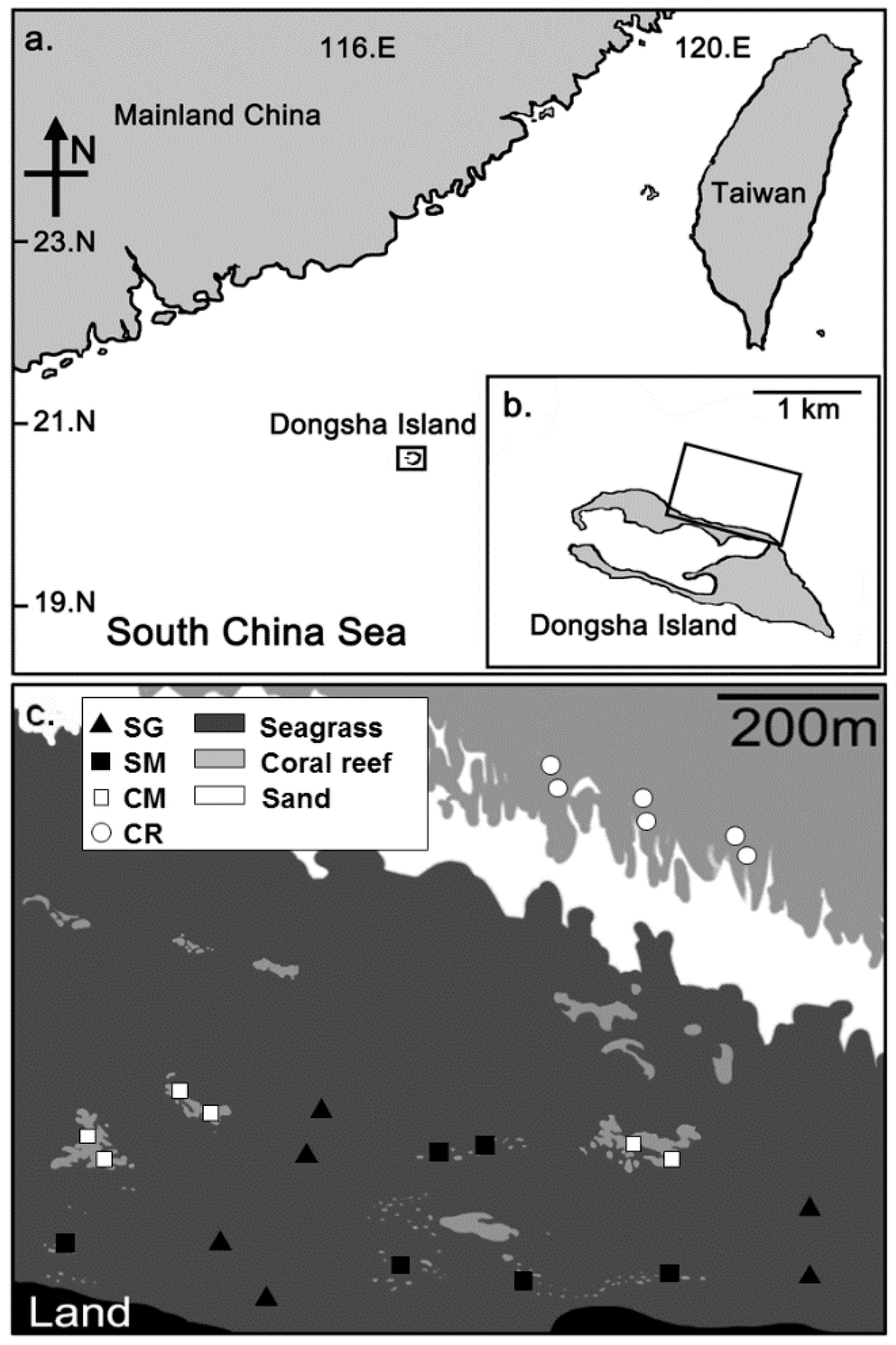
2.1. Study Site

Dongsha Island is a coral island with vast seagrass beds in South China Sea (Figure 1a,b; 20°43′ N, 116°42′ E). The island and neighboring atoll were incorporated into the Marine National Park and fishing activities have been prohibited since 2007. The total area of seagrass cover around Dongsha was found to be 8.2 km² [29]. The shallow northern waters (depth: 1–3 m) of Dongsha Island are often calm and clear and covered with high seagrass coverage (covering approximately 80–90% of the study area). Previous studies [30,31] showed a high abundance of reef fish, seagrass, and coral in the northern waters of Dongsha. Seagrass species in the canopies are mainly mixtures of Thalassia hemprichii, Cymodocea rotundata and Cymodocea serrulata. Some patchy coral reefs (volume: 1–100 m³) are scattered within the seagrass canopies (covering approximately 10% of the study area), forming various mixed habitats. Seagrass canopies extend 0.5–1.0 km from the shore, while pure coral reefs are approximately 0.6–1.5 km from the shore (Figure 1c).

Four different types of habitats were chosen as our study habitats (

Table 1. A conceptual image of the four habitat types and their characteristics in this study. The dark, grey, and white areas represent seagrass, reef corals, and sand, respectively.

Habitat Type	Side View	Top View	Seagrass Cover (%)	Hard Substrate Cover (%)
Seagrass beds (SG)			100%	0%
Seagrass-dominated mosaic habitats (SM)			50%	50% (live coral: 20–30%)
Coral-dominated mosaic habitats (CM)			10%	80% (live coral: 20–40%)
Coral reefs (CR)			0%	80% (live coral: 20–50%)

, Figure 1c). Our fieldworks were conducted in these four habitat types to compare the fish/invertebrate abundance and habitat structure within. The four habitat types were characterized by different seagrass-coral substrate compositions but had similar depths and seawater conditions: (1) Pure seagrass beds (SG), which featured nearly 100% seagrass cover without any hard coral or hard substrate present within a 100-m radius; (2) seagrass-dominated mixed habitats (SM), in which seagrass comprised approximately 50% of the benthic cover, with hard substrate comprising the other 50%. Of the hard substrate, stony corals (mainly Porites spp. and faviids) comprised 20–30% of the benthic cover, and these colonies were generally <0.5 m in height and <2 m³ in volume, and found within the seagrass canopy; (3) coral-dominated mixed habitats (CM), which were covered by approximately 10% seagrass canopy and 80% hard substrate. Of the hard substrate, live corals (large massive Porites spp., faviids and acroporids) and rubble comprised 20–40% and 50–70% of the benthic cover, respectively. The heights of the reef structures were >0.5 m and could exceed 1.3 m; (4) pure coral reefs (CR), were covered by approximately 80% hard substrate without any seagrass canopy present within a 200 m radius. Massive Porites spp., faviids and blue coral (Heliopora coerulea) were the dominant corals, and the heights of the reef structures were 1–2 m. The average live coral coverage was 20–30%, and rubble and sand comprised the remainder. The first three habitat types (SG, SM, CM) were 10–200 m from the shore, while the pure coral reef sites were approximately 800 m from the shore.

In total, eight surveys were conducted bimonthly only during the warm season (from April to October) in 2010 and 2011 to avoid intense northeastern monsoons during the cool season and coincide with the main recruitment season for reef fishes at Dongsha Island [30]. The surveys were conducted using six 20 × 2 m replicated transects that had been placed at one of six haphazardly chosen locations in each of the four habitat types (Figure 1c). The distance between different sampling habitat types were at least 50 m. All sampling transects in each habitat type were at least 5 m apart from each other. All transects were carefully placed and at least 10 min were allowed to pass between establishment of transects and the commencement of underwater visual census (UVC) survey (conducted on SCUBA) to limit disturbance to the fish. All four habitat types were surveyed during flood tides between 9 am and 4 pm to avoid confounding effects resulting from tidal and diel fauna movement [30]. In total, we collected 24 datasets (4 habitat types, each with 6 replicate transects) at each of the eight survey times, leading to a total of 192 data points used in the analyses described below.

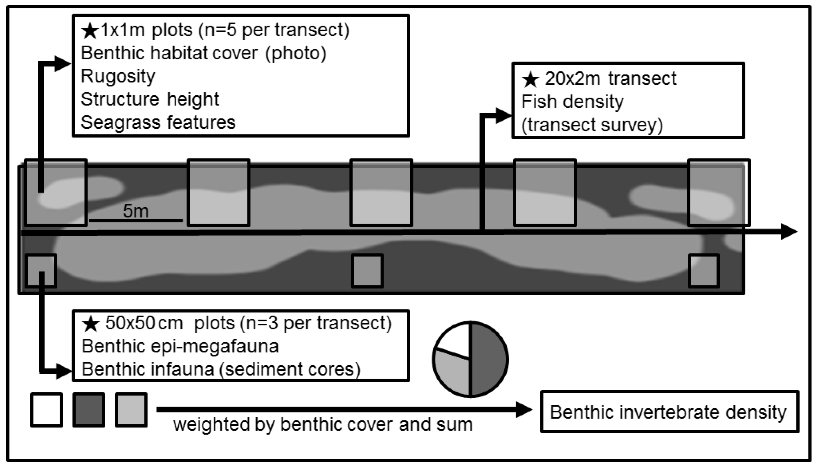
2.2. Habitat Structure

Seagrass variables (described below), live coral cover, structure heights, and habitat rugosity were measured in 1 × 1-m quadrats at five places (each 5-m apart) along each transect (Figure 2). Seagrass variables included shoot density, cover and leaf area index (LAI). Shoot density and cover data were derived from the seagrass survey by Huang et al. (2015) [31] at the same sites. LAI was calculated as the total leaf surface per unit area (m²) following Aioi & Pollard, 1993 [32]. The habitat rugosity was given one of the five scores based on the habitat assessment score by Gratwicke & Speight, 2005 [33]. Benthic substrate was photographed in the 1 × 1-m quadrats at five locations along each transect, and the planar areas of seagrass, live coral, and sand were quantified to percentage (%) with ImageJ 1.51K (National Institutes of Health, Bethesda, MA, USA) for further analysis described below.

2.3. Fish Surveys

The UVC surveys were conducted to record fish abundances, species diversity, and total body lengths (TL; to centimeter-level) along the 20 × 2 m transects in each habitat. To ensure the accuracy of size estimates, we practiced estimating fish lengths prior to the UVC surveys by estimating the lengths of objects of known size lying on the bottom (sensu Dorenbosch et al. (2005) [18]). All abundance data were standardized per unit area prior to analysis (individuals per 100 m²).

The four selected target carnivorous fish species: Lethrinus atkinsoni, Let. obsoletus, Let. harak (Lethrinidae) and Lutjanus fulviflamma (Lutjanidae) are all dominant carnivorous fish species around Dongsha Island [30], and they all clearly show ontogenetic habitat shifts from seagrass beds to coral reefs in their early life history stages [12,19,22]. We defined three body length categories to study ontogenetic habitat usage pattern according to our own and other previous studies [12,14,19]: (1) small (TL < 5 cm, newly recruited fish that feed mostly on small crustaceans), (2) medium (TL = 5–15 cm, juvenile stage, diets shift to large invertebrates, as mentioned below), and (3) large (TL > 15 cm, sub-adult to adult stage; [14,34]).

2.4. Diet Analysis

To identify the potential trophic competitors and predators of our target species, we have tried to examine the stomach contents of all the fish species within our study sites [30]. Fish diet samples were mainly derived from our previous study [30] and additional sampling during the study periods (Supplementary Table S1; Figure S1). The information for fish species that were present at our sites but we were unable to collect (Chaetodontidae, Pomacanthidae, Scaridae, and some cryptic species) was acquired from the FishBase website [35]. The compositions of the stomach contents were quantified according to Hyslop, 1980 [36] and expressed as a volume percentage (V%). To identify potential trophic competitors, we used Schoener’s index [37] of diet overlap to represent the trophic niche overlap between different fish species:

$${\mathrm{O}}_{ij}=1-0.5({\displaystyle \sum }\left|p_{ij}-p_{ik}\right|)$$

where p_ij and p_ik represent the proportions of food item i consumed by fish species j and k, respectively. This index ranges from 0 to 1, with higher values indicative of high levels of trophic niche overlap between species. We defined a priori that species with values greater than 0.6 had a significant diet overlap, and these species were considered to be potential trophic competitors with the target species [19,38,39]. There are about 200 reef fish species in our study area. We selected all species to examine the level of dietary overlap. However, species whose relative abundance <1% in the assemblage defined them as “rare species” were removed from the dietary overlap analyses. Since the diet habits of the target species differed among life history stages, the main competitors of each target species were also divided into the same three size classes (small, medium, and large) as used for the target species.

In terms of potential predators (i.e., piscivores), fish species with more than 10% (V%) of the stomach content being comprised (on average) of fish tissues were considered potential piscivores. Different sizes of piscivorous fish may feed on distinct fish prey. Some piscivores (herein referred to as “small piscivores”) only feed on larvae or post-settlement juvenile fish [40,41], whereas others prefer large-sized fish (herein referred to as “large piscivores” when fish with TL > 5 cm [>medium size] were present in their stomachs). Some fish species (e.g., lutjanids and sphyraenids) are small piscivores in their juvenile/sub-adult stages but become large piscivores in the adult stage.

2.5. Invertebrate Prey Abundance and Prey Availability

Benthic invertebrate abundances were quantified separately in the four habitats. Because different invertebrate fauna may prefer different substrates, epi-megafauna and small motile fauna were sampled at triplicate locations with distinct substrate surfaces (each at least 5-m apart) along each transect (Figure 2). For the sampling of epi-megafauna, we used 50 × 50 cm quadrats (n = 3) along each transect in each habitat type. All megafauna in quadrats were carefully collected, including sessile organism under rubbles. In terms of small motile fauna, we used stainless-steel cores (diameter = 7.6 cm) to collect sediment (with seagrass shoots) with 1 L of seawater at a depth of 10 cm on sandy bottom substrates. In some hard substrate habitats (e.g., rubble and coral), the aboveground structures were firstly captured by a plastic bag (planar area of 44.48 cm²) and were then smashed by a hammer after being collected in the plastic bag (also with 1 L of surrounding seawater at a depth of 10 cm). The organisms in the substrate samples were filtered through a 0.5 mm mesh, sorted, anesthetized using magnesium chloride or menthol, and fixed in 5% seawater-formalin for later species identification and quantification. Invertebrate abundances were presented by standardizing as specific densities (individuals per m²). The invertebrate density of each representative substrate surface in each of the four habitats was summed and weighed by the relative proportion of the substrate cover (calculated according to our imaging data described above) following the methods of Kramer et al. (2014) [42].

To quantify food availability, we estimated the amount of “available prey” for the four target fish species in each habitat type. “Major prey” that commonly occurred in the stomach contents (>20% of fish samples) and contributed, on average, more than 5% (V%) of the stomach contents of certain fish species were included in this analysis. Herein, we considered that the density of the target species and their trophic competitors may have influenced the amount of food available within a habitat. Therefore, the amount of available prey was calculated as follows: the total invertebrate prey density was divided by the sum of the density of the target species plus the density of their competitors [19]. Because different target fish species, as well as different size classes, have distinct diets and competitors, we calculated the food availability individually for each of the three size classes for each of the four target species.

2.6. Data Analysis

One-way ANOVAs were used to test the effects of habitat type on (1) the densities of potential piscivores and competitors, (2) the abundance of invertebrate prey, and (3) habitat structure. For invertebrate prey densities, only large crustaceans (mostly decapods) and small crustaceans (such as amphipods, copepods, and tanaids) were considered in the model since they were the main food sources of the four target fish species [30]. All data were tested for homogeneity of variance by Levene’s tests, and a log or square root transformation was employed if necessary before analysis in SPSS 12.0 (Polar Engineering and Consulting, Chicago, IL, USA). If the data still showed heterogeneity of variance after transformation, Gabriel or Games–Howell post hoc tests were used to determine the differences among the habitats. Since fish density and available prey data were heteroscedastic and non-normally distributed, we used 2-factor permutational multivariate analysis of variance (PERMANOVA) to determine the differences in the densities of fish and available prey of the four target species in the three body length categories (fixed factors: Small, medium, and large) among the four habitat types (fixed factors: Seagrass, seagrass-dominated mosaic habitat, coral-dominated mosaic habitat, and coral reef). Data sets were log-transformed to down-weigh the influence of high values before analysis. Because the PERMANOVA revealed no significant differences in fish assemblages (p = 0.947), fish densities (p = 0.521), and invertebrate density (p = 0.089) between sampling times, data from the same habitat type were pooled for the following analyses. Euclidean distance was then used to generate a resemblance distance matrix, and pairwise tests were used to determine the differences between habitats if significant differences were detected.

A distance-based redundancy analysis (dbRDA) ordination diagram was used to reveal the target fish habitat usage throughout ontogeny among the four habitats. Fish assemblage data were log (x + 1) transformed to reduce the influence of dominant species before analysis, and a resemblance matrix using Bray-Curtis similarity was generated. The densities of target fish in three body length categories were used as predictor variables in the dbRDA ordination diagram. The statistics above were computed using PRIMER 6.1.13 and PERMANOVA+ [43,44].

A generalized linear model (GLM) with a bootstrap selection process was used to find the major drivers of habitat usage pattern by the four target species. Poisson and negative binomial data distribution assumptions were chosen in our analysis. The densities of three size categories of these four target species were examined with a combination of factors (habitat type (ratio of seagrass bottom: reef substrate bottom), prey density, food availability, competitor density, and piscivore density) in the regression models. The null model (no factor selected) and alternative models (combinations of all factors) were compared with Akaike’s information criterion (AIC) using a stepwise algorithm (stepAIC) in the MASS package of the R program. The model with the lowest AIC value was determined to represent the best fit, and the chosen factors were determined to be the major contributors to habitat usage pattern by the target fishes. Fish sampling and experiments were approved and permitted by the Marine National Park Headquarters of Taiwan (No. 98415).

3. Results

3.1. Habitat Structure Features

The habitat structure features differed significantly across the four habitat types (

Table 2. Testing the effect of habitat type (n = 4 classifications; see Figure 1.) on select biological variables with one-way ANOVA followed by Tukey’s post-hoc tests (*** p < 0.001; * p < 0.05). Habitat abbreviations: Seagrass beds (SG), seagrass-dominated mosaic habitats (SM), coral-dominated mosaic habitats (CM), and coral reefs (CR).

Variable	F Statistic	Post-hoc Differences
Seagrass density	52327.24 ***	SG > SM > CM > CR
Seagrass leaf area index (LAI)	858.80 ***	SG, SM > CM > CR
Seagrass cover	22088.20 ***	SG > SM > CM > CR
Live coral cover	437.05 ***	CR, CM > SM > SG
Structure height	2433.20 ***	CR > CM > SM, SG
Structure rugosity	438.92 ***	CR > CM > SM > SG
Large crustacean density	67.75 ***	CM > SG, SM, CR
Small crustacean density	0.55	None
Large piscivore density	4.32 *	CR > SG, SM, CM
Small piscivore density	84.31 ***	SM, CM > CR > SG
Potential competitor density	415.36 ***	CM > SM, CR > SG

; Figure 3). The pure seagrass habitats had higher seagrass density and seagrass cover but lower rugosity than the other three habitats. The habitats with corals had significantly higher structural rugosity, as well as structure height. Our results showed higher piscivore densities in the three coral-associated habitats than in the pure seagrass beds (Figure 4a). The densities of small piscivores were dramatically higher in both the two mosaic habitats than in pure seagrass and coral habitats (Table 2). The densities of large piscivorous fish were highest in the pure coral habitats. The pure seagrass habitats had the lowest densities of both large and small piscivorous fish.

For benthic invertebrates, crustaceans were the most dominant taxa and contributed approximately 67.06% to the total abundance, followed by polychaetes (27.14%) and gastropods (1.39%). Amphipods (53.08%) and copepods (35.30%) were the most abundant crustaceans. Large crustaceans (mostly decapods) constituted only a small proportion (4.66%) of the total abundance. The densities of small crustaceans were not significantly different among the four habitats (Figure 4b, Table 2). However, the densities of large crustaceans were higher in the mosaic habitats than in pure seagrass and coral habitats (Figure 4b). The seagrass habitat had the lowest density of large crustaceans among the four habitats.

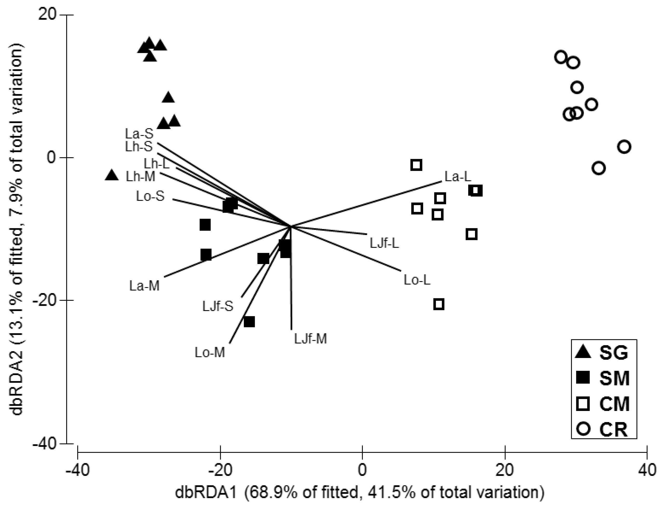
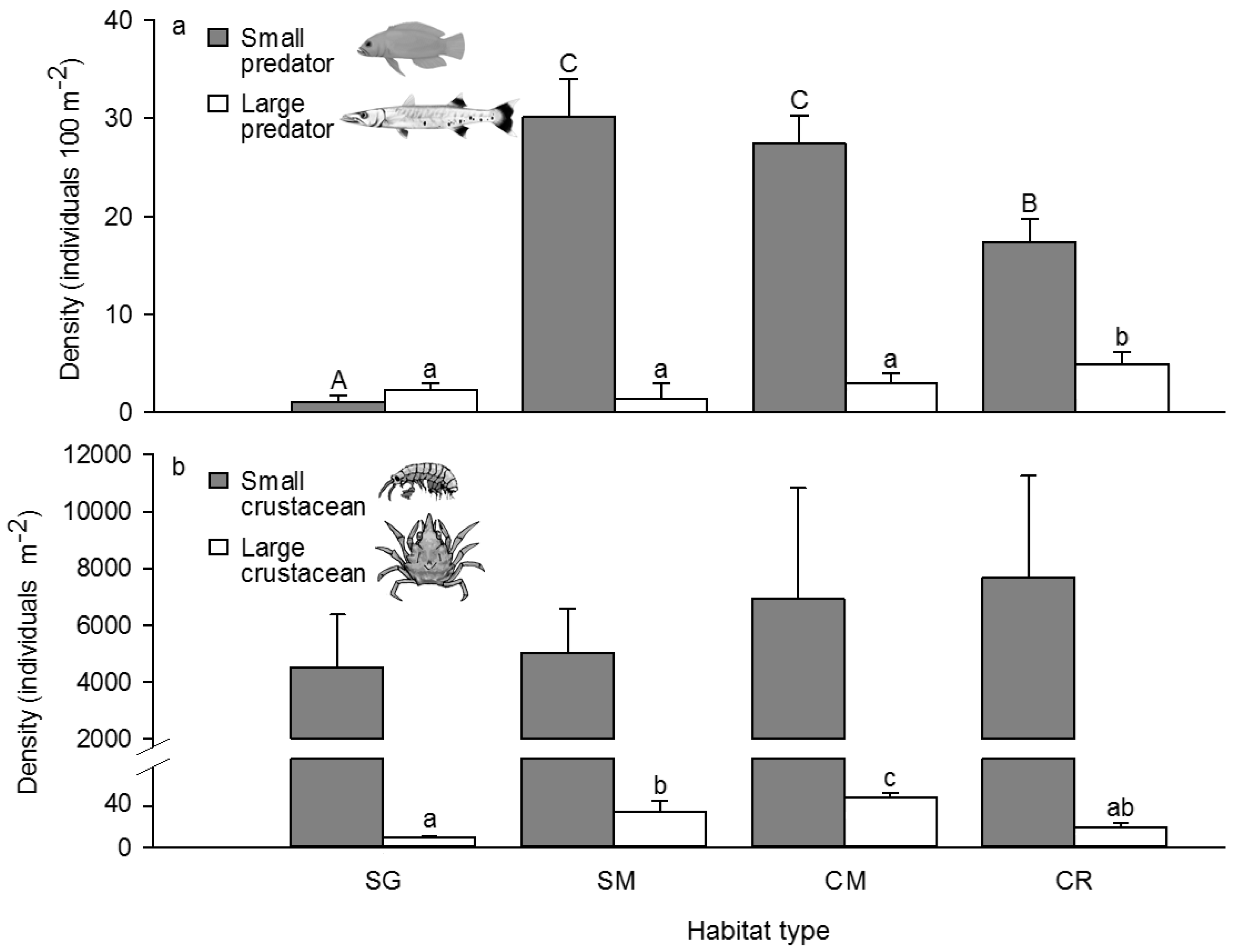
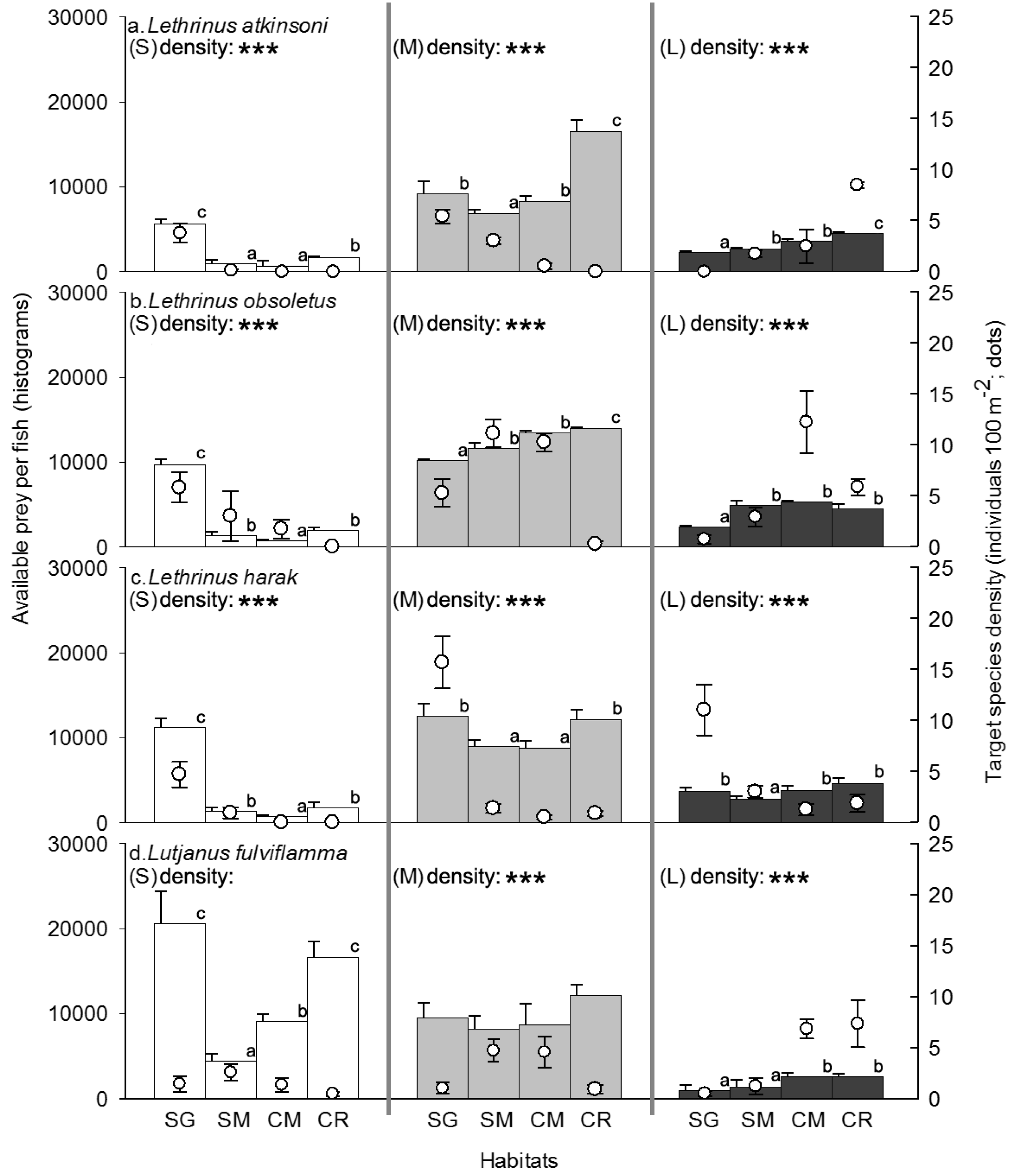
3.2. Competitor, Food Availability, and Habitat Usage Pattern of the Target Fish Species

The four target fish species fed mostly on crustaceans (

Table 3. Diet composition (V%) of the four target species in three different total length (small, medium, and large) categories (“n” = sample size). Abbreviations for food items: Fi: Fish, De: Decapod, Is: Isopod, Os: Ostracod, Am: Amphipod, Ta: Tanaid, Co: Copepod, Ga: Gastropod, Bi: Bivalve, Po: Polychaete, Ec: Echinoid, and Dt: Detritus.

Species	n	Fi	De	Is	Os	Am	Ta	Co	Ga	Bi	Po	Ec	Dt
Lethrinus atkinsoni
Small	26		1		3	27	7	60			2
Medium	11		83	2		9		1	2	2	1
Large	22		88	1					7	2	1	1
Lethrinus obsoletus
Small	28		1		2	6	13	77			1
Medium	30	3	78	1		6		4	1	1	5	1
Large	19	8	84	1		1		1	2		3
Lethrinus harak
Small	32		6		3	15	38	37			1
Medium	33		87	1	1	2			2		6	1
Large	22	6	87	1					1	1	3	1
Lutjanus fulviflamma
Small	24	1	26	1		34	14	21					2
Medium	19	4	74	1	1	7	2	10	1		1
Large	21	21	77	1									1

). The three lethrinids fed exclusively on small crustaceans (e.g., copepods and amphipods) when their body sizes were small, while they shifted their diet to large crustaceans (decapods) after they reached medium size. Lut. fulviflamma fed on both large (27%) and small (70%) crustaceans when they were small, switching to large crustaceans (70–80%) after they reached medium size.

We found several fish species that showed a high diet overlap, and these species were considered by Schoener’s index to be the potential competitors of our target species (

Table 4. Schoener’s index indicating the trophic niche overlaps among 1) the four target species in three different life history stages indexed by total length (S: Small, M: Medium, and L: Large) and 2) other potential competitors. Only index values greater than 0.60 have been shown.

Family	Species	La-S	La-M	La-L	Lo-S	Lo-M	Lo-L	Lh-S	Lh-M	Lh-L	LJf-S	LJf-M	LJf-L
Lethrinidae	Lethrinus atkinsoni (La-S)
	L. atkinsoni (La-M)
	L. atkinsoni (La-L)		0.89
	Lethrinus obsoletus (Lo-S)	0.76
	L. obsoletus (Lo-M)		0.89	0.83
	L. obsoletus (Lo-L)		0.88	0.89
	Lethrinus harak (Lh-S)
	L. harak (Lh-M)		0.89	0.93		0.88	0.91
	L. harak (Lh-L)		0.86	0.91		0.87	0.96		0.93
Lutjanidae	Lutjanus fulviflamma (LJf-S)
	L. fulviflamma (LJf-M)		0.75	0.75		0.77	0.78		0.76	0.78
	L. fulviflamma (LJf-L)		0.77			0.81	0.87		0.79	0.86		0.74
Apogonidae	Ostorhinchus spp.	0.72			0.87			0.60
	Cheilodipterus quinquelineatus	0.63			0.78
Labridae	Stethojulis strigiventer	0.86			0.71			0.69
	Halichoeres spp.	0.78						0.86			0.68
	Choerodon anchorago		0.65	0.65		0.68			0.64
Nemipteridae	Scolopsis lineata (S)	0.94			0.73			0.68
	S. lineata (M)	0.82			0.70			0.70
Pomacentridae	Abudefduf spp.	0.63			0.67
	Chrysiptera spp.	0.73			0.60			0.61
	Dischistodus prosopotaenia	0.68			0.74

). High diet overlap (70–90%) was detected between the medium and large sizes of the four target species, while rather low diet overlap was recorded in the small sizes of the target species (except for between small Let. obsoletus and Let. atkinsoni [76%]). Other fish species, such as apogonids, labrids, nemipterids, and pomacentrids, showed a high diet overlap with the small lethrinids. Choerodon anchorago instead showed a high dietary overlap with the medium and large lethrinids. The diets of individuals of all three size classes of Lut. Fulviflamma, in contrast, did not overlap appreciably with other sampled fish species. Potential competitors of the other target fish species were significantly more abundant in coral-associated habitats than in seagrass beds (Table 2). Coral-dominated mosaic habitats harbored the highest densities of potential competitors (9.95 ± 3.54 m⁻²), while seagrass beds had the lowest (0.81 ± 0.07 m⁻²).

We found that the densities of the four target species increased when the prey density or food availability increased (i.e., target species density and food availability were positively correlated). The GLM stepwise multiple regression results (

Table 5. The results of the generalized linear model (GLM) indicating the best fit model and the factors (habitat type, prey density, food availability, competitor density, and piscivore density) affecting the densities of the four target fishes across three different life history stages (small, medium, and large). AIC = Aikake’s information criterion.

Species/Size	Best Fit Model	AIC
Lethrinus atkinsoni
Small	prey density + food availability + piscivore density	42.92
Medium	habitat type + prey density	78.68
Large	habitat type + prey density + competitor density + food availability	104.5
Lethrinus obsoletus
Small	habitat type + piscivores density	99.06
Medium	prey density + competitor density + food availability	119.24
Large	habitat type + prey density + competitor density + food availability	139.02
Lethrinus harak
Small	habitat type + prey density + competitor density + food availability + piscivores density	62.42
Medium	habitat type + prey density + food availability	105.03
Large	prey density + competitor density + food availability	119.24
Lutjanus fulviflamma
Small	habitat type	105.12
Medium	habitat type + prey density + competitor density + food availability	139.73
Large	habitat type + prey density + food availability	139.69

) showed that invertebrate prey densities and food availability best explained the habitat usage pattern by most lethrinids and medium/large-sized Lut. fulviflamma. Competitor densities also likely influenced the densities of large-sized Let. atkinsoni, small/large-sized Let. harak, medium/large-sized Let. obsoletus, as well as medium-sized Lut. fulviflamma. Piscivore densities affected only the three small-sized categories of the target lethrinids and did not affect Lut. fulviflamma.

The densities of competitors and invertebrate prey contributed to the differences in food availability for the four target species among the four habitats (Figure 5). The PERMANOVA results revealed that the densities and abundance of available prey of the four target species were significantly different among habitats (p < 0.05), with the exception of Lut. fulviflamma, which showed no significant difference in the abundance of available prey among habitats (p = 0.116). The three lethrinids likely used seagrass beds that had significantly higher prey availability (p = 0.001). Let. atkinsoni (Figure 5a) and Let. obsoletus (Figure 5b) showed clear ontogenetic habitat shifts from pure seagrass to coral-associated habitats after the species reached medium size. Small-sized Let. atkinsoni and Let. obsoletus were mostly found in seagrass habitats. The large-sized Let. atkinsoni and Let. obsoletus showed clear habitat usage pattern for coral-dominated habitats over pure seagrass habitats. On the other hand, Let. harak showed no ontogenetic habitat shifts (Figure 5c). All sizes of this species likely used pure seagrass habitats, where prey availability was highest for small and medium-sized Let. harak; in contrast, prey availability for large members of this species was similar across habitats.

Small-sized Lut. fulviflamma exhibited no significant habitat usage pattern, while medium-sized and large individuals likely used mosaic and coral-dominated habitats, respectively (Figure 5d). Prey availability for small Lut. fulviflamma was higher in both pure seagrass and pure coral reef habitats, while prey availability for the medium and large-sized individuals was significantly lower in seagrass beds compared to the other three habitat types.

4. Discussion

Habitat structure along a gradient of seagrass and coral varied, and each of the four habitat types likely offered different habitat functions and services for the target fish species. We found higher fish and invertebrate density in the two mixed habitats compared to the pure seagrass and coral habitats; such has been documented previously [18,26,27]. The reason behind this could be due to the diversity of mosaic habitats within which shelter could be sought, or, alternatively, the increase in connectivity between coral reefs and seagrass beds [1,2,25]. The presence of coral patches/reef in a seagrass canopy clearly enhanced the three-dimensional structure, rugosity, and, consequently, the number (and complexity) of crevices and hiding places. As a result, these mosaic habitats that are more complex when compared to pure seagrass beds.

We found that crustaceans, which are the main food resources of three Lethrinus species and Lutjanus fulviflamma, were distinctly distributed among the four habitats. The three habitats featuring live coral had more large crustaceans (e.g., decapods) than the pure seagrass beds. Coral reefs tend to harbor higher densities of large crustaceans than seagrass or sandy habitats (

Table 6. Comparisons of benthic invertebrate density (per m²) among various habitat types, as determined by previous studies. Abbreviations: SC: Small crustaceans (amphipods, ostracods, copepods, and tanaids), LC: large crustaceans (decapods), AC: Sum of all crustaceans and All: Sum of all benthic invertebrates.

Habitat Type	Sand	Seagrass	Seagrass-Coral Mixed	Rubble	Live Coral	Reference
Iriomote, Ryukyu Islands	SC: 6500 LC: 0 All: 11000	SC: 10000 LC: 180 All: 24000			SC: 4000 LC: 400 All: 12000	[15]
Ishigaki, Ryukyu Islands		SC: 20000 LC: 350			SC: 20000 LC: 200	[21]
Dakwan, Southern Taiwan	SC: <10 LC: <5 All: 10	SC: 30 LC: 10 All: 50			SC: 80 LC: 18 All: 120	[25]
Dongsha Island, South China Sea	SC: 100 LC: <5	SC: 4000 LC: 20	SC: 5000–7000 LC: 40–50	SC: 4000–8000 LC: 20–30	SC: 5000–7000 LC: 20	this study
Lizard Island, GBR	AC: 5000			AC: 230000	AC: 66	[47]
Kunduchi, Tanzania		SC: 20 LC: <10			SC: 40 LC: 50	[12]
Playa Larga Reef, Panama				All: 200-500	All: 400–1600	[17]

), presumably due to their structural complexity [16,42,45]. Such enhanced habitat surface area is associated with higher densities of the predominant food sources of crustaceans, including detritus, periphyton, and macroalgae [42,46]. Nakamura & Sano (2005) [15] and Lee & Lin (2015) [19] both found that coral substrate hosts more decapods than adjacent seagrass beds. On the other hand, a seagrass canopy not only provides heterogeneous habitats for decapods but may also yield organic matter that is utilized as food for decapods [47,48]. The structural complexity of coral reefs, as well as the high organic matter content of seagrass beds, might explain why large crustaceans were more abundant in mixed habitats than in pure seagrass and coral habitats.

In contrast to the large crustaceans, no distinct differences in the densities of small crustaceans were found across the four habitat types. Although previous studies have found that coral habitats are characterized by higher densities of small crustaceans than seagrass beds (Table 6), we found that the high covered seagrass beds around Dongsha Island could support as many small crustaceans as the nearby coral reefs; such was also observed by Nakamura et al. (2012) [22]. A luxuriant seagrass canopy can also act as a filter to capture small planktonic animals or organic particles in the water column [49,50]. Moreover, the large amount of seagrass detritus accumulated in the sediments of seagrass beds [31], as well as the two mixed habitats may also have served as important food sources and shelter for small detritivorous crustaceans [51].

Two mosaic and pure coral habitats were found to have more piscivorous fishes, especially small piscivores, than the pure seagrass habitats. Small piscivores are normally benthic dwellers and can influence reef fish recruitment given their preference for recruit-sized fish [40,41,52]. Coral reefs are known to have high abundance and species richness of small piscivores, which leads to higher juvenile mortality in coral habitats than in the neighboring seagrass habitats for many fish species [12,20,21,22]. The densities of these small piscivores were five to eight times higher in the mixed reef habitats than in the pure seagrass habitats, and approximately 1.5 times higher in the coral-dominated mosaic habitats than in the coral reef habitats at Dongsha Island. This may be because seagrass-coral mosaic habitats offer more shelter and higher food availability for these small piscivores. The piscivore distribution patterns revealed that the potential predation pressures may be higher in the habitats in which corals were present than in the seagrass beds, leading to a higher predation risk for the small-sized juvenile fish in these coral and mosaic habitats.

According to the GLM results, the piscivore density affected the habitat usage of lethrinids in only the small-sized categories. Thus, most small fish of our target species may have shown habitat usage pattern for pure seagrass beds given the low densities of their predators there. Prey availability is also an important factor affecting habitat usage for small lethrinids. Their density was mostly positively correlated with prey availability. Previous studies noted that habitats with higher food supplies could lead to higher growth rates for juvenile reef fishes [12,22], and we found that some fish species avoid coral habitats since the abundance of trophic competitors may result in lower food availability [19]. Indeed, competition can significantly influence the food resources for individual fish within the same habitat [53]. For small lethrinids, small benthic crustaceans were the most important food sources. Other crustacean feeding fishes may be the main trophic competitors for the small-sized lethrinids at Dongsha Island. The occurrence of these competitors in coral-associated habitats may decrease the availability of food for the target species [19,39]. To avoid competition, the small-sized lethrinids may preferentially inhabit seagrass habitats in order to seek a greater food supply. Prey availability may also have affected the habitat usage patterns of lethrinid species after reaching medium size. The three lethrinid species mostly fed on large crustaceans, and their diets were ~90% similar to each other. We found that each fish species had its own habitat usage strategy for optimizing food acquisition and reducing resource competition. Let. atkinsoni and Let. obsoletus showed greater ontogenetic habitat shifts to reef-associated mosaic habitat than Let. harak. Let. harak has a high growth rate compared to other lethrinids [34] and may primarily occupy seagrass habitats. Thus, the habitat shifts of Let. atkinsoni and Let. obsoletus appear linking to the higher prey availability on coral reefs [19,22] to decrease the potential for trophic or space competition with Let. harak in pure seagrass beds. We surmise that the mosaic habitats may provide a diversity of resources, so that species in similar trophic guilds could nevertheless occupy different niches (e.g., by diversifying their habitat choices).

Unlike lethrinids, Lut. fulviflamma likely used mosaic habitats over pure seagrass beds when they were in both small and medium-sized. Their ontogenetic shift to coral-featured habitats may be linked to the higher availability of decapod food sources at such habitats. The early development of the digestive system of Lut. fulviflamma allows for the consumption of hard-shelled animals and even juvenile fish [54]. As a result, food may not be a limiting factor in habitat usage pattern by Lut. fulviflamma. Habitat type showed an influencing factor for only the small-sized Lut. fulviflamma. We believe that sheltering structures might be favored by the small-sized Lut. fulviflamma since they actively forage after dusk and rest in sheltered areas during the daytime [55]. Hence, the coral and seagrass mosaic habitats offer not only quality hiding places during the day, but also potential foraging grounds at night.

5. Conclusions

Our results—derived from seagrass beds, seagrass-coral mosaic habitats, and coral reefs within the same seascape—provide insight into the early habitat usage pattern of carnivorous reef fishes. The four dominant juvenile carnivorous fishes showed distinct ontogenetic habitat usage patterns based on the food availability in seagrass and coral mosaic habitats. The mosaic habitats certainly offered high abundances of large crustaceans but also more predators and trophic competitors. Juvenile carnivorous fishes may shelter in pure seagrass habitats to avoid predation and/or competition when they were small in size. After exceeding medium sizes, they exhibited species-specific habitat usage patterns in order to optimize feeding in seagrass-coral mosaic habitats. Our results revealed different carnivorous fish species would use mosaic habitats in different ontogenetic stages. We suggest that seagrass-coral mosaic habitats may offer not only habitats, but also support additional ecological function for reef fishes. Many carnivorous fishes obtain their food needs as their sizes increase. The mosaic habitats can therefore be critical transitional habitats for shelters, foraging grounds, and/or even connection joints for them in coastal systems. Moreover, four dominant target fish species showed distinct ontogenetic habitat usage patterns based on the food availability in mosaic habitats. These patterns indicate that mosaic habitats may offer a wide range of trophic niche for similar guilds to coexist within a similar seascape of seagrasses and reefs, increasing the biodiversity of coastal systems. The seagrass-coral mosaic habitats are common habitats in tropical coastal systems. Their ecological function or connection for reef fishes may have been overlooked previously as we know little about these heterogeneous habitat complexes at a microhabitat scale. For conservation, it is worthwhile to protect these mosaic habitats in order to maintain the crucial habitats and connection in tropical coastal systems.

References

1. Olds, A.D.; Connolly, R.M.; Pitt, K.A.; Maxwell, P.S. Primacy of seascape connectivity effects in structuring reef fish assemblages. Mar. Ecol. Prog. Ser. 2012, 462, 191–203. [Google Scholar] [CrossRef]
2. Berkström, C.; Lindborg, R.; Thyresson, M.; Gullström, M. Assessing connectivity in a tropical embayment: Fish migrations and seascape ecology. Biol. Conserv. 2013, 166, 43–53. [Google Scholar] [CrossRef]
3. Nagelkerken, I.; Sheaves, M.; Baker, R.; Connolly, R.M. The seascape nursery: A novel spatial approach to identify and manage nurseries for coastal marine fauna. Fish Fish. 2015, 16, 362–371. [Google Scholar] [CrossRef]
4. Eggertsen, L.; Ferreira, C.E.L.; Fontoura, L.; Kautsky, N.; Gullström, M.; Berkström, C. Seaweed beds support more juvenile reef fish than seagrass beds in a south-western Atlantic tropical seascape. Estuar. Coast. Shelf Sci. 2017, 196, 97–108. [Google Scholar] [CrossRef]
5. Tano, S.A.; Eggertsen, M.; Wikström, S.A.; Berkström, C.; Buriyo, A.S.; Halling, C. Tropical seaweed beds as important habitats for juvenile fish. Mar. Freshwater Res. 2017, 68, 1921–1934. [Google Scholar] [CrossRef]
6. Nagelkerken, I. Evaluation of nursery function of mangroves and seagrass beds for tropical decapods and reef fishes: And underlying mechanisms. In Ecological Connectivity among Tropical Coastal Ecosystems; Nagelkerken, I., Ed.; Springer: Dordrecht, The Netherlands, 2009; pp. 357–399. [Google Scholar]
7. Nyström, M.; Folke, C. Spatial resilience of coral reefs. Ecosystems 2001, 4, 406–417. [Google Scholar] [CrossRef]
8. Mumby, P.J.; Hastings, A. The impact of ecosystem connectivity on coral reef resilience. J. Appl. Ecol. 2008, 45, 854–862. [Google Scholar] [CrossRef]
9. McCook, L.J.; Almany, G.R.; Berumen, M.L.; Day, J.C.; Green, A.L.; Jones, G.P.; Leis, J.M.; Planes, S.; Russ, G.R.; Sale, P.F.; et al. Management under uncertainty: Guide-lines for incorporating connectivity into the protection of coral reefs. Coral Reefs 2009, 28, 353–366. [Google Scholar] [CrossRef]
10. Dahlgren, C.P.; Eggleston, D.B. Ecological processes underlying ontogenetic habitat shifts in a coral reef fish. Ecology 2000, 81, 2227–2240. [Google Scholar] [CrossRef]
11. Almany, G.R. Differential effects of habitat complexity, predators and competitors on abundance of juvenile and adult coral reef fishes. Oecologia 2004, 141, 105–113. [Google Scholar] [CrossRef]
12. Kimirei, I.A.; Nagelkerken, I.; Trommelen, M.; Blankers, P.; Van Hoytema, N.; Hoeijmakers, D.; Huijbers, C.M.; Mgaya, Y.D.; Rypel, A.L. What drives ontogenetic niche shifts of fishes in coral reef ecosystems? Ecosystems 2013, 16, 783–796. [Google Scholar] [CrossRef]
13. Wen, C.K.; Almany, G.; Williamson, D.; Pratchett, M.; Jones, G. Evaluating the effects of marine reserves on diet, prey availability and prey selection by juvenile predatory fishes. Mar. Ecol. Prog. Ser. 2012, 469, 133–144. [Google Scholar] [CrossRef]
14. Wilson, S.K.; Depczynski, M.; Holmes, T.H.; Noble, M.M.; Radford, B.T.; Tinkler, P.; Fulton, C.J. Climatic conditions and nursery habitat quality provide indicators of reef fish recruitment strength. Limnol. Oceanogr. 2017, 62, 1868–1880. [Google Scholar] [CrossRef]
15. Nakamura, Y.; Sano, M. Comparison of invertebrate abundance in a seagrass bed and adjacent coral and sand areas at Amitori Bay, Iriomote Island, Japan. Fish. Sci. 2005, 71, 543–550. [Google Scholar] [CrossRef]
16. Enochs, I.C. Motile cryptofauna associated with live and dead coral substrates: Implications for coral mortality and framework erosion. Mar. Biol. 2012, 159, 709–722. [Google Scholar] [CrossRef]
17. Nakamura, Y.; Sano, M. Overlaps in habitat use of fishes between a seagrass bed and adjacent coral and sand areas at Amitori Bay, Iriomote Island, Japan: Importance of the seagrass bed as juvenile habitat. Fish. Sci. 2004, 70, 788–803. [Google Scholar] [CrossRef]
18. Dorenbosch, M.; Grol, M.G.G.; Nagelkerken, I.; van der Velde, G. Distribution of coral reef fishes along a coral reef-seagrass gradient: Edge effects and habitat segregation. Mar. Ecol. Prog. Ser. 2005, 299, 277–288. [Google Scholar] [CrossRef]
19. Lee, C.L.; Lin, H.J. Ontogenetic habitat utilization patterns of juvenile reef fish in low predation habitats. Mar. Biol. 2015, 162, 1799–1811. [Google Scholar] [CrossRef]
20. Grol, M.G.G.; Dorenbosch, M.; Kokkelmans, E.M.; Nagelkerken, I. Mangroves and seagrass beds do not enhance growth of early juveniles of a coral reef fish. Mar. Ecol. Prog. Ser. 2008, 366, 137–146. [Google Scholar] [CrossRef]
21. Grol, M.G.G.; Nagelkerken, I.; Rypel, A.L.; Layman, C.A. Simple ecological trade-offs give rise to emergent cross-ecosystem distributions of a coral reef fish. Oecologia 2011, 165, 79–88. [Google Scholar] [CrossRef] [PubMed]
22. Nakamura, Y.; Hirota, K.; Shibuno, T.; Watanabe, Y. Variability in nursery function of tropical seagrass beds during fish ontogeny: Timing of ontogenetic habitat shift. Mar. Biol. 2012, 159, 1305–1315. [Google Scholar] [CrossRef]
23. Dorenbosch, M.; Grol, M.G.G.; Groene, A.; van der Velde, G.; Nagelkerken, I. Piscivore assemblages and predation pressure affect relative safety of some back-reef habitats for juvenile fish in a Caribbean bay. Mar. Ecol. Prog. Ser. 2009, 379, 181–196. [Google Scholar] [CrossRef]
24. Sheaves, M. Consequences of ecological connectivity: The coastal ecosystem mosaic. Mar. Ecol. Prog. Ser. 2009, 391, 107–115. [Google Scholar] [CrossRef]
25. Ries, L.; Fletcher, R.J.; Battin, J.; Sisk, T.D. Ecological responses to habitat edges: Mechanisms, models, and variability explained. Ann. Rev. Ecol. Syst. 2004, 35, 491–522. [Google Scholar] [CrossRef]
26. Dorenbosch, M.; Grol, M.G.G.; Nagelkerken, I.; van der Velde, G. Different surrounding landscapes may result in different fish assemblages in East African seagrass beds. Hydrobiologia 2006, 563, 45–60. [Google Scholar] [CrossRef]
27. Tuya, F.; Vanderklift, M.A.; Wernberg, T.; Thomsen, M.S. Gradients in the number of species at reef-seagrass ecotones explained by gradients in abundance. PLoS ONE 2011, 6, e20190. [Google Scholar] [CrossRef] [PubMed]
28. Hylkema, A.; Vogelaar, W.; Meesters, H.W.G.; Nagelkerken, I.; Debrot, A.O. Fish species utilization of contrasting sub-habitats distributed along an ocean-to-land environmental gradient in a tropical mangrove and seagrass lagoon. Estuar. Coast 2015, 38, 1448–1465. [Google Scholar] [CrossRef]
29. Lin, H.J.; Hsieh, L.Y.; Liu, P.J. Seagrasses of Tongsha Island, with descriptions of four new records to Taiwan. Bot. Bull. Acad. Sin. 2005, 46, 163–168. [Google Scholar]
30. Lee, C.L.; Huang, Y.H.; Chung, C.Y.; Lin, H.J. Tidal variation in fish assemblages and trophic structures in tropical Indo-Pacific seagrass beds. Zool. Stud. 2014, 53, 56. [Google Scholar] [CrossRef]
31. Huang, Y.H.; Lee, C.L.; Chung, C.Y.; Hsiao, S.C.; Lin, H.J. Carbon budgets of multispecies seagrass beds at Dongsha Island in the South China Sea. Mar. Environ. Res. 2015, 106, 92–102. [Google Scholar] [CrossRef]
32. Aioi, K.; Pollard, P.C. Biomass, leaf growth and loss rate of the seagrass Syringodium isoetifolium on Dravuni Island, Fiji. Aquat. Bot. 1993, 46, 283–292. [Google Scholar] [CrossRef]
33. Gratwicke, B.; Speight, M.R. The relationship between fish species richness, abundance and habitat complexity in a range of shallow tropical marine habitats. J. Fish Biol. 2005, 66, 650–667. [Google Scholar] [CrossRef]
34. Ebisawa, A.; Ozawa, T. Life-history traits of eight Lethrinus species from two local populations in waters off the Ryukyu Islands. Fish. Sci. 2009, 75, 553–566. [Google Scholar] [CrossRef]
35. Froese, R.; Pauly, D. FishBase. World Wide Web electronic publication, version 2012. Available online: www.fishbase.org (accessed on 1 June 2012).
36. Hyslop, E.J. Stomach contents analysis: A review of methods and their application. J. Fish Biol. 1980, 17, 411–429. [Google Scholar] [CrossRef]
37. Schoener, T.W. Nonsynchronous spatial overlap of lizards in patchy habitats. Ecology 1970, 51, 408–418. [Google Scholar] [CrossRef]
38. Sala, E.; Ballesteros, E. Partitioning of space and food by three fish of the genus Diplodus (Sparidae) in a Mediterranean rocky infralittoral ecosystem. Mar. Ecol. Prog. Ser. 1997, 152, 273–283. [Google Scholar] [CrossRef]
39. Nagelkerken, I.; van der Velde, G.; Verberk, W.C.E.P.; Dorenbosch, M. Segregation along multiple resource axes in a tropical seagrass fish community. Mar. Ecol. Prog. Ser. 2006, 308, 79–89. [Google Scholar] [CrossRef]
40. Almany, G.R.; Webster, M.S. The predation gauntlet: Early post-settlement mortality in reef fishes. Coral Reefs 2006, 25, 19–22. [Google Scholar] [CrossRef]
41. Feeney, W.E.; Lönnstedt, O.M.; Bosiger, Y.; Martin, J.; Jones, G.P.; Rowe, R.J.; McCormick, M.I. High rate of prey consumption in a small predatory fish on coral reefs. Coral Reefs 2012, 31, 909–918. [Google Scholar] [CrossRef]
42. Kramer, M.J.; Bellwood, D.R.; Bellwood, O. Benthic Crustacea on coral reefs: A quantitative survey. Mar. Ecol. Prog. Ser. 2014, 511, 105–116. [Google Scholar] [CrossRef]
43. Clarke, K.R.; Gorley, R.N. PRIMER v6: User Manual/Tutorial; PRIMER-E: Plymouth, UK, 2006. [Google Scholar]
44. Anderson, M.J.; Gorley, R.N.; Clarke, K.R. PERMANOVA+ for PRIMER: Guide to Software and Statistical Methods; PRIMER-E: Plymouth, UK, 2008. [Google Scholar]
45. Enochs, I.C.; Toth, L.T.; Brandtneris, V.W.; Afflerbach, J.C.; Manello, D.P. Environmental determinants of motile cryptofauna on an eastern Pacific coral reef. Mar. Ecol. Prog. Ser. 2011, 438, 105–118. [Google Scholar] [CrossRef]
46. Glynn, P.W.; Enochs, I.C. Invertebrates and their roles in coral reef ecosystems. In Coral Reefs: An Ecosystem in Transition; Dubinsky, Z., Stambler, N., Eds.; Springer: Dordrecht, The Netherlands, 2011; pp. 273–325. [Google Scholar]
47. Peduzzi, P.; Herndl, G.J. Decomposition and significance of seagrass leaf litter (Cymodocea nodosa) for the microbial food web in coastal waters (Gulf of Trieste, Northern Adriatic Sea). Mar. Ecol. Prog. Ser. 1991, 71, 163–174. [Google Scholar] [CrossRef]
48. Lepoint, G.; Cox, A.S.; Dauby, P.; Poulicek, M.; Gobert, S. Food sources of two detritivore amphipods associated with the seagrass Posidonia oceanica leaf litter. Mar. Biol. Res. 2006, 2, 355–365. [Google Scholar] [CrossRef]
49. Parrish, J.D. Fish communities of interacting shallow-water habitats in tropical oceanic regions. Mar. Ecol. Prog. Ser. 1989, 58, 143–160. [Google Scholar] [CrossRef]
50. Macreadie, P.I.; Hindell, J.S.; Keough, M.J.; Jenkins, G.P.; Connolly, R.M. Resource distribution influences positive edge effects in a seagrass fish. Ecology 2010, 91, 2013–2021. [Google Scholar] [CrossRef] [PubMed]
51. Dimech, M.; Borg, J.A.; Schembri, P.J. Motile macroinvertebrate assemblages associated with submerged Posidonia oceanica litter accumulations. Biol. Mar. Medit. 2006, 13, 130–133. [Google Scholar]
52. Ritchie, E.G.; Johnson, C.N. Predator interactions, mesopredator release and biodiversity conservation. Ecol. Lett. 2009, 12, 982–998. [Google Scholar] [CrossRef]
53. Hixon, M.A.; Jones, G.P. Competition, predation, and density-dependent mortality in demersal marine fishes. Ecology 2005, 86, 2847–2859. [Google Scholar] [CrossRef]
54. Nanami, A.; Shimose, T. Interspecific differences in prey items in relation to morphological characteristics among four lutjanid species (Lutjanus decussatus, L. fulviflamma, L. fulvus and L. gibbus). Environ. Biol. Fishes 2013, 96, 591–602. [Google Scholar] [CrossRef]
55. Dorenbosch, M.; Verweij, M.C.; Nagelkerken, I.; Jiddawi, N.; van der Velde, G. Homing and daytime tidal movements of juvenile snappers (Lutjanidae) between shallow-water nursery habitats in Zanzibar, western Indian Ocean. Environ. Biol. Fishes 2004, 70, 203–209. [Google Scholar] [CrossRef]
Figure 1. The location of (a) Dongsha Island in the South China Sea, (b) the study area (square inset) on the northern coast of Dongsha Island, and (c) the locations of the 24 study sites, which spanned seven habitat structure categories (defined in the legend).
Diversity 11 00025 g001
Figure 2. The survey/sampling design of each transect in each habitat type (n = 6/habitat type × 4 habitat types × 8 sampling/survey times = 192 transect surveys).
Diversity 11 00025 g002
Figure 3. Distance-based redundancy analysis (dbRDA) showing the ordination of four habitat types by four target fish species’ densities in three body length categories. The abbreviations for the four habitats can be found in Table 1. The abbreviations of fish species and body length categories are La: Lethrinus atkinsoni, Lo: Lethrinus obsoletus, Lh: Lethrinus harak, and LJf: Lutjanus fulviflamma. S: Small, M: Medium, and L: Large.
Diversity 11 00025 g003
Figure 4. Densities of (a) piscivorous fish and (b) crustacean invertebrate prey in the four habitat types (see Table 1 for abbreviations). The values represent means ± SE. The letters above the histograms denote post-hoc differences (capital letters for small predator and crustacean; lowercase letter for large predator and crustacean), if an overall difference was detected in the ANOVA (see Table 2).
Diversity 11 00025 g004
Figure 5. Available prey (histograms and left axes) and densities (dots and right axes) for the four target species—(a) Lethrinus atkinsoni, (b) Lethrinus obsoletus, (c) Lethrinus harak, and (d) Lutjanus fulviflamma—in three body length categories (S: small, M: medium, and L: large). The values represent means ± SE. The letters above the histograms denote the pairwise differences (*** p < 0.001) in available prey if an overall difference was detected in the PERMANOVA model. The abbreviations for the four habitats can be found in Table 1.
Diversity 11 00025 g005