Abstract
The peninsula effect is a biological diversity pattern found in peninsulas in which the number of species decreases toward the tip of the peninsula. The geometry hypothesis, as one proposed cause of the peninsula effect, attempts to predict this pattern by examining the peculiarities of peninsular geometry. As peninsulas are characterized by their isolated positions, it has been suggested that a decreased immigration-to-extinction rate is the cause of the decrease in species diversity from the base to the tip of a peninsula. We aimed to test the geometry hypothesis on tree species in the Florida peninsula by modeling the latitudinal abundance pattern using sample-based tree inventory data. We postulated that the current abundance distribution of a species is a ramification of past immigration–extinction dynamics in a peninsula, as well as an important indicator of such dynamics in the future. The latitudinal abundance patterns of 113 tree species in Florida in the southeastern United States were simulated with the Huisman–Olff–Fresco (HOF) model using the USDA Forest Service’s Forest Inventory and Analysis (FIA) database. Evidence species for the geometry hypothesis were then selected if the simulated latitudinal abundance pattern was asymmetric with its abundance maxima occurring within the Florida peninsula (i.e., approximately 31.5° latitude or lower). Our HOF model results found that most species (87% of 113 species) did not experience any steep abundance decline along the Florida peninsula when compared with their general trend across the range, suggesting that the observed diversity pattern of tree species in Florida could merely be a continuation of latitudinal diversity gradients in the southeastern United States, independent of peninsular geometry.
1. Introduction
The study of species diversity patterns and their underlying factors has been a continuing scientific inquiry for the past century (e.g., [1,2,3,4,5,6]). On the continental scale, a latitudinal diversity gradient (LDG) is a primary diversity pattern recognized in a wide spectrum of taxa in which the highest levels of species density (i.e., gamma diversity for a region, [7]) are seen in the tropics, while declining toward polar regions [4,5,8]. The underlying mechanisms of LDG are generally well explained by various factors, including hypotheses based on environment [9], evolutionary factors [10], and history [11]; however, regional scale anomalies—in particular, the inverse LDG pattern found on peninsulas—remain unresolved [12].
Since the first observation of the decreasing diversity of bird species along the Florida peninsula [13], this monotonic pattern has attracted considerable attention over the past 60 years. In particular, tree species in the Florida peninsula exhibit an inverse LDG pattern, such that the number of species within a defined area—i.e., species richness as a proxy for tree species diversity—decreases from a broad mainland base toward the narrow, southern tip of the peninsula. Although the diversity pattern of woody plants has received little attention, these plants are among the most prominent organisms that sustain the biodiversity and functions of ecosystems.
Simpson [14] first postulated the “peninsula effect” observed in mammalian species, suggesting that the geometry of peninsulas surrounded by the ocean limits the immigration of species and increases extinction rates (hereafter referred to as the “geometry hypothesis”), causing a decrease in diversity from the base to the tip of a peninsula. This geometry hypothesis, thus, emphasizes the role of the island-like geometry of peninsulas on population dynamics (i.e., an imbalance of the immigration/extinction rates). The term “peninsula effect” has commonly been used to denote a process that explains the diversity pattern found within peninsulas; however, there is great disagreement relative to the causative processes of such patterns [15]. Herein, the use of the term “peninsula effect” only refers to the monotonic decreasing diversity pattern along the peninsula’s axis, and any mechanism-related proposal is described as an individual hypothesis meant to explain the decreasing diversity pattern of the peninsula effect.
Support for the geometry hypothesis includes studies of birds in Baja California, in Florida, and in Yucatan (Mexico) [16], amphibians and reptiles in the Florida peninsula [7], six vertebrate groups (lizards, snakes, birds, mammals in general, and heteromyid rodents and bats) in the Baja California peninsula [17], forest vegetation in the state of Maine [18], and passerine birds in Spain [19]. At the same time, mixed patterns have been observed in peninsulas: hump-shaped species richness of ground beetles in the mid-range of the Florida peninsula [20] and no pattern related to scorpions along the axis of the Baja California peninsula [21] or in the tropical forests of Belize and Venezuela [22]. A noteworthy summary was a meta-analysis by Jenkins et al. [23], in which only 18 out of 37 studies (49%) exhibited the peninsula effect, and the geometry hypothesis is considered as an idiosyncratic phenomenon that depends on context, taxonomic group, and analytic scales [12,23].
While a variety of mobile species with tracked movement would be well tested by the geometry hypothesis, tree species have not been extensively studied because they exhibit a delayed reaction to the environment, with a varying dispersal mode that is difficult to be monitored. In addition, this lag time, together with a large range size, makes tree species difficult to study in terms of immigration/extinction rate.
Alternatively, tree species abundance distributions from a systematic, sample-based inventory, such as Forest Inventory and Analysis (FIA) data, may provide insights for assessing immigration/extinction dynamics, as they are closely related under the umbrella of population dynamics. Empirical studies from invasion ecology have shown that high abundance is significantly associated with successful immigration and establishment, and low abundance can lead to high levels of extinction [24,25,26]. Therefore, we postulate that the current abundance distribution of a species is a ramification of past immigration/extinction dynamics in a peninsula, as well as an important indicator of such dynamics in the future. Furthermore, we predict an appreciable, abrupt decrease in the abundance pattern when a species range enters the Florida peninsula if a tree species has been experiencing declining immigration/extinction rates because of peninsular geometry.
The objective of this study was to evaluate the peninsula effect for tree species richness and geometry hypothesis as an underlying cause in the Florida peninsula. Analytically, we examined the species-level latitudinal abundance pattern in the context of latitudinal diversity gradient for Florida. Specifically, we adopted the standardized simulation approach implemented in Huisman–Olff–Fresco (HOF) models [27] to detect the abundance variations of each species in Florida with respect to its entire range. As supporting evidence for the geometry hypothesis, we looked for tree species with signatures of steep abundance decreases as they entered the Florida peninsula.
2. Materials and Methods
In the United States (US), the FIA program of the United States Department of Agriculture (USDA) Forest Service provides consistent nationwide tree census information regarding the extent, condition, status, and trends of the country’s forest resources [28]. The FIA program relies on a systematic, five-year rolling annual inventory system with a unified, fixed-radius plot design, which lends significant credibility in terms of the timeliness of data acquisition and comparability [29]. The FIA plot consists of four 7.2-meter fixed-radius subplots to tally all trees with a diameter at breast height (dbh) of at least 12.7 centimeters (cm), and each subplot contains a microplot for seedlings and understory inventory.
In this study, we retrieved the most recent FIA annual inventory (from 2010 to 2015) for 31 eastern states, comprising a total of 118,092 tree records from 77,523 inventory plots in the FIA database (FIADB) version 6.0 (available at https://apps.fs.usda.gov/fia/datamart/datamart_access.html). Issues with perturbed (fuzzed and swapped) FIA plot locations representing privately owned land were negligible in this study, as they were aggregated at a much larger area of 20 km × 20 km grids [30,31]. The bay area of Monroe county, Florida was not surveyed by the FIA program because the southern tip of Florida does not meet the FIA standards for forest classification.
As a basic analytic unit, we overlaid an array of 20 km × 20 km grids over the study area of 31 eastern US states, resulting in a total of 7320 grids (approximately 3.01 million km2), of which 570 grids correspond to the Florida peninsula (Figure 1). This grid size was adopted from the size of estimation unit of FIA sampling framework [32]. Firstly, we estimated grid-level species richness (i.e., counts of unique tree species) following Kwon et al. [33] in two steps: first, we selected grids containing more than three plots and, second, we applied a bootstrapping method of 1000 iterations to calculate the mean values for species counts after randomly selecting three plots for each grid. This method ensures that our sample-based richness estimates were not biased by the area sampled (i.e., the number of plots within a grid) because the relationship between the number of plots and the richness in a grid was linear (Pearson’s r of 0.58, p < 0.01). These grid-level species richness values were then tabulated to the nearest 1° latitudinal band to construct latitudinal richness patterns (gamma diversity sensu Whittaker [34]; Magurran [35]).
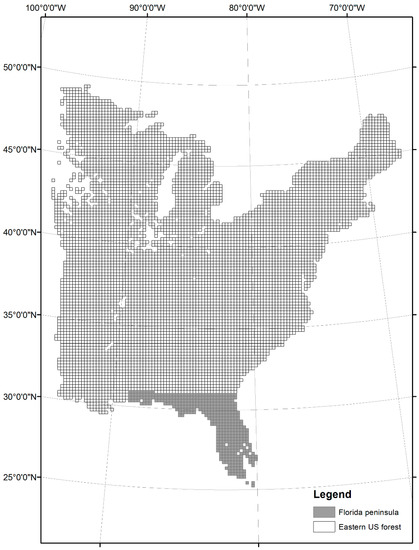
Figure 1.
The study area of 31 eastern US states overlaid with an array of 20 km × 20 km grids (7320 grids) as an analytic unit. Shaded grids represent Florida peninsula (570 grids).
Next, to examine species-level abundances, we tabulated the sum of the absolute stem counts per species for each grid by accounting for actual plot size sampled using a per-acre tree expansion factor (variable code TPA stored in the TREE table of the FIADB), resulting in standardized stem counts per one-acre area. We then examined individual species-level abundance patterns along the latitudinal gradients. That is, for each species, we computed its mean stem counts across the range using a 1° moving window, such that for each 0.5° of latitude, the mean absolute stem count in a window (±0.5° latitudinal bands) was extracted. HOF models, which compensate for a small sample size using a bootstrapping technique [36], were then applied to simulate the abundance pattern of each species along the latitudinal gradients.
HOF models (Figure 2) are a set of five hierarchical logistic regression models that were originally used for fitting a unimodal species response curve on an environmental gradient. A HOF model generates five pre-determined model outputs with decreasing complexity: skewed (type V), symmetric (type IV), plateau (type III), monotonic (type II), and flat response (type I) [37]. Beginning with the most complex model (type V), the most appropriate model is selected based on the likelihood ratio test of residual deviance with a significance level of p = 0.05.
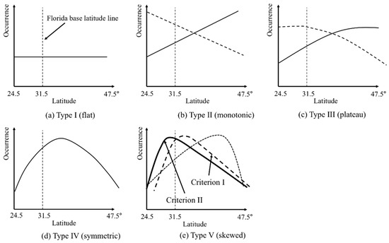
Figure 2.
Five Huisman–Olff–Fresco (HOF) model output types; (a) type I flat response; (b) type II monotonic (north and south are represented by solid and dashed lines, respectively); (c) type III plateau (north and south are represented by solid and dashed lines, respectively); (d) type IV symmetric; (e) type V as skewed (north and south are represented by solid and dashed lines, respectively). Criterion I is type V with a south skewness maximum represented by a dashed line in figure (e), and criterion II is a subset of criterion I with maxima occurring lower than the 31.5° latitude.
HOF model-based evidence for the geometry hypothesis was based on the following two criteria: the first was HOF model type V with a southern skewness (i.e., model maxima occurring in the southern latitudinal range center; criterion I), because we expected that an abrupt decline of abundance, due to peninsular geometry, would lead to an asymmetric abundance curve with a skewness toward the peninsula direction. Second, among species satisfying criterion I, the HOF model maxima occurred lower than the 31.5° latitude (criterion II), which is the approximate latitude of the peninsula base, because we speculated that if the maxima occurred farther north from the peninsula base, its asymmetric decline (type V) might be associated with other stochastic factors, such as disturbances, rather than the geometry hypothesis. This latter criterion can be considered a conservative approach to evaluating the geometry hypothesis.
The other HOF model types (I to IV) were not regarded as evidence for geometry hypothesis, as these types were not related to abrupt abundance changes, thus not suggesting an imbalance of immigration/extinction rates in the peninsula. In addition, tree species with less than a 5° latitude range (the difference between the minimum and maximum latitudes) were regarded as endemic species and, thus, omitted from the HOF model simulation because they were not pertinent to the population dynamics relative to peninsular geometry.
Data from the FIADB were processed using PostgreSQL 9.6.1 [38], and all statistical analyses were performed in R version 2.12.1 [39].
3. Results
A total of 252 tree species across 31 eastern states were identified from the FIADB, and 113 species (representing 29 taxonomic families and 62 genera) were observed at a lower 31.5° latitude in the Florida peninsula alone. Tree species richness showed a hump-shaped pattern along the latitudinal gradient in the eastern US with the highest (142 species) being around mid-range latitude (35 to 40° latitude) and decreases in both directions, the lowest (31 species) being located in the southern tip of Florida (Figure 3). The richness pattern within the Florida peninsula exhibited strong gradual monotonic declines from the base (latitude 31.5°) to the tip (latitude 25°), demonstrating a clear peninsula effect (Pearson’s correlation between species richness and latitude was 0.96; p < 0.01).
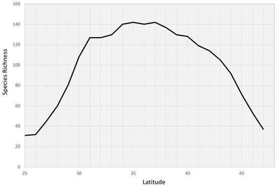
Figure 3.
Tree species richness from the Forest Inventory and Analysis database (FIADB) along the latitudinal gradients.
The latitudinal pattern of abundance (i.e., absolute mean stem counts) for 113 tree species in Florida exhibited a full spectrum of HOF model responses (see Table S1 in the Supplementary Material). Table 1 shows a summary of abundance distribution for 113 Florida tree species, as simulated by the HOF models. Type V (skewed) was the most common latitudinal abundance pattern, while type III (plateau) was the least common.

Table 1.
All Florida species described by HOF model types or endemic status and top five abundance species in each category.
There were 21 endemic species in Florida, mostly in southern Florida and sparsely distributed across the range, thus excluded from the HOF model. Among the 92 general (non-endemic) species, seven (7.6%) were flat response, as fitted by the HOF model type I, and 26 species (28.3%) were monotonic response (type II). Thirteen of the type II species (14.1%) showed a linear abundance pattern that increased southward, and the other thirteen were in the north. Three species (3.3%) exhibited a plateau pattern of type III, two of which had maxima in the north of the range’s center, with the other one being south of the range center. Thirteen species (14.1%) showed maxima occurring at the center of the range, as fitted by a symmetric Gaussian response (type IV). Within type V (skewed), which included 43 (43.7%) of the total general species, 21 species had their peak abundance north of the latitudinal center of the range; however, eleven of them extended their range into Canada, thus, the northern skewness was not derived from their entire range (see Table S1 in the Supplementary Material).
The HOF model output types explained, thus far, type I to type V of north maxima were not considered evidence species for the geometry hypothesis because they were not related to an abrupt abundance decrease pattern in the peninsula. Twenty-two type V species (23.9%) had their peak abundance south of the latitudinal center of the range (type V of south maxima), satisfying criterion I as evidence in support of the geometry hypothesis. Among those criterion I species, the abundance maxima of 12 species (13% out of 92 general species) were near the Florida peninsula base and lower (criterion II), supporting the peninsula geometry hypothesis in Florida (Table 2), while the other 10 were located farther north on the mainland. Our analysis therefore suggested that there is an insufficient number of evidence species (13%) to support the geometry hypothesis when examined by the latitudinal abundance pattern in the Florida peninsula.
Table 2.
Evidence species (criterion II) supporting the geometry hypothesis for the peninsula effect.
4. Discussion
We examined the latitudinal abundance pattern of individual tree species in Florida using simulated unimodal species response curves implemented using the HOF model to uncover potential evidence for the geometry hypothesis in the Florida peninsula. Our analysis found only 12 species (13% of 92 species) with an abrupt steep abundance decline along the peninsula as evidence for the geometry hypothesis. This may mean that, first, the geometry hypothesis is not a valid explanation for tree species in Florida or, second, that population dynamics are difficult to trace by the current abundance pattern. Lastly, it could mean that tree species richness gradients in the Florida peninsula are merely driven by environmental factors specific to this region, such as forest patch size or other limiting factors (e.g., frost days, forest area, and precipitation in the driest quarter; see Kwon et al. [33]).
Yet, those 12-evidence species (Table 2) deserve conservation consideration because, with marked abrupt abundance attrition, these species may be more susceptible to various biotic and abiotic disturbances (e.g., outstanding climate change, hurricane, wildfire, insect infestation, or land fragmentation). Also, five of these 12-evidence species (Celtis laevigata, Nyssa biflora, Pinus clausa, Pinus elliottii, Salix bonplandiana) were identified by Murphy et al. [40] as having an overall range deduction as examined by the proportion of occupied cells as a response to contemporary climate change. Our analysis indicated that these evidence species have experienced an outstanding stress in the region thus a potential for range shrinkage.
Seven species met criterion I (type V of south skewedness) but not criterion II (abundance maxima occurring below the 31.5° latitude). Three were oak species (Quercus pagoda, Quercus lyrata, Quercus nigra), while the other four were Juniperus virginia, Pinus taeda, Liquidambar styraciflua, and Cornus florida. These seven species demonstrated abundance maxima (their population source latitude) unrestricted by the peninsula; thus, peninsular geometry seemed to play a less important role in the decline of their abundance in Florida, but they still have a potential for range shrinkage. In total, 11 of the 19 Quercus genera species found in Florida which met at least one of the criteria, suggesting the need for monitoring efforts in support of conservation.
Although not meeting our criteria for abrupt abundance decline in the peninsula, 62 species experienced progressive abundance attrition (type II north, type III north, and type IV and type V south) in Florida, and this species-level phenomenon might be responsible for the overall tree richness pattern observed in Florida. A similar conclusion was drawn for the diversity pattern of birds in the Iberian Peninsula by Carrascal and Diaz [41]. In addition, although 21 species with less than a 5° latitude range were excluded from our analysis; those endemic species deserve conservation efforts to ensure they adapt to their small-size niches in changing environments.
4.1. Comparison with Other Peninsula Effect Studies
Although woody plant species have rarely been tested for the geometry hypothesis of the peninsula effect in North America, we discuss our findings in light of other relevant studies. A study by Schwartz [42] investigated the clumping of tree species range termini to infer the peninsula effect by using a diversity measure derived from Little’s historical tree species range maps [43] and reported no overall diversity decline for a total of 222 species in Florida. However, of these 222 species, our study only observed 72 of them in the FIADB, and they showed a strong richness decline towards the tip of the peninsula. On the other hand, when temperate and tropical species were examined separately, Schwartz [42] found that the temperate species exhibited the peninsula effect, while the tropical species showed an inverse pattern. Following their classification of temperate and tropical species, we also found that the temperate species in the FIADB exhibited the peninsula effect, while tropical affinity showed no decreasing pattern towards the tip of the peninsula. In addition, Schwartz [42] observed dramatic species composition change from northern to southern Florida but, in our study, the species pool change represented by the FIA inventory was not as appreciable, as identified by Schwartz. A disagreement between Schwartz [42] and our study was unsurprising because, as we suspect, the disagreement is mainly attributable to the different data source for Little’s range map [43], which approximated natural distributions of woody plants, while the FIA inventory is based on sample plots in forest lands confined to fixed-radius subplots.
A study by Milne and Forman [18] concluded that reduced land area was a causative explanation for the slight overall peninsula effect in the woody vegetation of Maine. However, their study combined data from multiple adjacent and small peninsulas in the region and focused on alpha diversity rather than gamma diversity (as was used in our study). Kwon et al. [33] also found forest patch areas and frost days as the most determinative factors behind tree species richness in Florida using spatial modeling approaches, and the geometry hypothesis, as tested by the nearby waterbody area, was not a significant factor.
4.2. Thoughts Regarding Other Hypotheses for the Peninsula Effect in Florida
The history and habitat hypotheses have also been proposed for the peninsula effect in other regions [44,45]. Florida’s geological history has been relatively simple and stable since the early Pliocene Epoch [46], and this long environmental stability can be assumed to have minimized the impact of past climatic or geological events, such as glaciers, on the current distribution of tree species. This long environmental stability also implies that tropical regions can contain more specialized species with smaller niches, thereby allowing for greater diversity where resources are fairly abundant throughout the year [6]. This assumption is supported by our observation that 21 endemic Florida species had their entire range (≤5° latitude) in Florida, while only six species with less than a 5° latitude were found above the 32° latitude; this ecological phenomenon is also known as Rapoport’s rule [47]. Thus, the history hypothesis can explain why there are many endemic species in the Florida peninsula, but it is not sufficient to address the causal factors for the peninsula effect. Regarding habitat hypotheses, climate conditions change from warm and temperate in the north of Florida to subtropical in the south, and it is likely that the climatic and habitat conditions control the peninsula effect in Florida [33]. The present study, however, attempted to test the geometry hypothesis only, as no other studies quantified the potential effect of peninsula geometry in tree species population dynamics due to limited empirical evidence [23,48].
5. Conclusions
We investigated the geometry hypothesis for the peninsula effect using simulated latitudinal abundance patterns for 113 tree species in Florida. We found that only 12 species out of 92 non-endemic species showed an abrupt steep abundance decline along the Florida peninsula when compared with their general trend across the range. Although not conclusive evidence, this result suggests that the observed richness pattern of tree species in Florida could merely be a continuation of latitudinal diversity gradients in the southeastern US, independent of peninsular geometry. However, those 12-evidence species, as well as seven criterion I species, indicate that they have experienced outstanding stress in the region such that a monitoring effort is needed to support population conservation.
Supplementary Materials
The following are available online at http://www.mdpi.com/1424-2818/11/2/20/s1, Table S1: HOF model results for 92 (non-endemic) species.
Author Contributions
Conceptualization, Y.K.; methodology, Y.K.; L.F.; software, Y.K.; L.F.; validation, Y.K.; L.F.; formal analysis, Y.K.; L.F.; investigation, Y.K.; L.F.; resources, Y.K.; L.F.; data curation, Y.K.; L.F.; writing—original draft preparation, Y.K.; L.F.; writing—review and editing, Y.K.; L.F.; visualization, Y.K.; L.F.; supervision, Y.K.; project administration, Y.K.; funding acquisition, Y.K.; L.F.
Funding
The authors received no specific funding for this work.
Conflicts of Interest
The authors declare no conflict of interest.
References
- Gleason, H.A. On the relation between species and area. Ecology 1922, 3, 158–162. [Google Scholar] [CrossRef]
- Fisher, R.A. Allowance for double reduction in the calculation of genotype frequencies with polysomic inheritance. Ann. Eugen. 1943, 12, 169–171. [Google Scholar] [CrossRef]
- Rohde, K. Latitudinal gradients in species diversity: The search for the primary cause. Oikos 1992, 65, 514–527. [Google Scholar] [CrossRef]
- Rosenzweig, M.L. Species Diversity in Space and Time; Cambridge University Press: Cambridge, UK, 1995. [Google Scholar]
- Blackburn, T.M.; Gaston, K.J. Spatial patterns in the species richness of birds in the New World. Ecography 1996, 19, 369–376. [Google Scholar] [CrossRef]
- Willig, M.R.; Kaufman, D.M.; Stevens, R.D. Latitudinal gradients of biodiversity: Pattern, process, scale, and synthesis. Annu. Rev. Ecol. Evol. Syst. 2003, 34, 273–309. [Google Scholar] [CrossRef]
- Kiester, A.R. Species density of North American amphibians and reptiles. Syst. Zool. 1971, 20, 127–137. [Google Scholar] [CrossRef]
- Brown, J.H.; Lomolino, M.V. Biogeography, 2nd ed.; Sinauer: Sunderland, MA, USA, 1998. [Google Scholar]
- Wang, Z.; Fang, J.; Tang, Z.; Lin, X. Patterns, determinants and models of woody plant diversity in China. Proc. R. Soc. Lond. B Biol. Sci. 2010, 278. [Google Scholar] [CrossRef]
- Condamine, F.L.; Sperling, F.A.H.; Wahlberg, N.; Rasplus, J.; Kergoat, G.J. What causes latitudinal gradients in species diversity? Evolutionary processes and ecological constraints on swallowtail biodiversity. Ecol. Lett. 2012, 15, 267–277. [Google Scholar] [CrossRef]
- Mittelbach, G.G.; Schemske, D.W.; Cornell, H.V.; Allen, A.P.; Brown, J.M.; Bush, M.B.; Harrison, S.P.; Hurlbert, A.H.; Knowlton, N.; Lessios, H.A.; et al. Evolution and the latitudinal diversity gradient: Speciation, extinction and biogeography. Ecol. Lett. 2007, 10, 315–331. [Google Scholar] [CrossRef]
- Battisti, C. Peninsular patterns in biological diversity: Historical arrangement, methodological approaches and causal processes. J. Nat. Hist. 2014, 48, 2701–2732. [Google Scholar] [CrossRef]
- Robertson, W.B. An analysis of the breeding-bird populations of tropical Florida in relation to the vegetation. Ph.D. Thesis, University of Illinois Urbana-Champaign, Urbana, IL, USA, 1955. [Google Scholar]
- Simpson, G.G. Species density of North American recent mammals. Syst. Zool. 1964, 13, 57–73. [Google Scholar] [CrossRef]
- Olivier, P.I.; Rolo, V.; Van Aarde, R.J. Pattern or process? Evaluating the peninsula effect as a determinant of species richness in coastal dune forests. PLoS ONE 2017, 12, e0173694. [Google Scholar] [CrossRef]
- MacArthur, R.H.; Wilson, E.O. The Theory of Island Biogeography; Princeton University Press: Princeton, NJ, USA, 1967. [Google Scholar]
- Taylor, R.J.; Regal, P.J. The peninsular effect on species diversity and the biogeography of Baja California. Am. Nat. 1978, 112, 583–593. [Google Scholar] [CrossRef]
- Milne, B.T.; Forman, R.T.T. Peninsulas in Maine: Woody plant diversity, distance, and environmental patterns. Ecology 1986, 67, 967–974. [Google Scholar] [CrossRef]
- González-Taboada, F.; Nores, C.; Ángel Álvarez, M. Breeding bird species richness in Spain: Assessing diversity hypothesis at various scales. Ecography 2007, 30, 241–250. [Google Scholar] [CrossRef]
- Peck, S.B.; Larivee, M.; Browne, J. Biogeography of ground beetles of Florida (Coleoptera: Carabidae): The peninsula effect and beyond. Ann. Entomol. Soc. Am. 2005, 98, 951–959. [Google Scholar] [CrossRef]
- Due, A.D.; Polis, G.A. Trends in scorpion diversity along the Baja California peninsula. Am. Nat. 1986, 128, 460–468. [Google Scholar] [CrossRef]
- Tackaberry, R.; Kellman, M. Patterns of tree species richness along peninsular extensions of tropical forests. Glob. Ecol. Biogeogr. Lett. 1996, 5, 85–90. [Google Scholar] [CrossRef]
- Jenkins, D.G.; Rinne, D. Red herring or low illumination? The peninsula effect revisited. J. Biogeogr. 2008, 35, 2128–2137. [Google Scholar] [CrossRef]
- Colautti, R.I.; Grigorovich, I.A.; MacIsaac, H.J. Propagule pressure: A null model for biological invasions. Biol. Invasions 2006, 8, 1023–1037. [Google Scholar] [CrossRef]
- Lavergne, S.; Molina, J.; Debussche, M.A.X. Fingerprints of environmental change on the rare mediterranean flora: A 115-year study. Glob. Chang. Biol. 2006, 12, 1466–1478. [Google Scholar] [CrossRef]
- Sutton, F.M.; Morgan, J.W. Functional traits and prior abundance explain native plant extirpation in a fragmented woodland landscape. J. Ecol. 2009, 97, 718–727. [Google Scholar] [CrossRef]
- Huisman, J.; Olff, H.; Fresco, L.F.M. A hierarchical set of models for species response analysis. J. Veg. Sci. 1993, 4, 37–46. [Google Scholar] [CrossRef]
- Smith, W.B. Forest inventory and analysis: A national inventory and monitoring program. Environ. Pollut. 2002, 116, S233–S242. [Google Scholar] [CrossRef]
- Bechtold, W.A.; Patterson, P.L. The Enhanced Forest Inventory and Analysis Program: National Sampling Design and Estimation Procedures; US Department of Agriculture Forest Service, Southern Research Station: Asheville, NC, USA, 2005. [Google Scholar]
- Gibson, J.; Moisen, G.; Frescino, T.; Edwards, T.C. Using publicly available forest inventory data in climate-based models of tree species distribution: Examining effects of true versus altered location coordinates. Ecosystems 2014, 17, 43–53. [Google Scholar] [CrossRef]
- Prisley, S.P.; Wang, H.-J.; Radtke, P.J.; Coulston, J. Combining FIA plot data with topographic variables: Are precise locations needed? In Forest Inventory and Analysis (FIA) Symposium 2008; October 21–23, 2008; Park City, UT Proc RMRS-P-56CD; US Department of Agriculture, Forest Service, Rocky Mountain Research Station: Fort Collins, CO, USA, 2009; Available online: https://www.fs.fed.us/rm/pubs/rmrs_p056.pdf (accessed on 29 January 2019).
- McRoberts, R.E.; Bechtold, W.A.; Patterson, P.L.; Scott, C.T.; Reams, G.A. The enhanced Forest Inventory and Analysis program of the USDA Forest Service: Historical perspective and announcement of statistical documentation. J. For. 2005, 103, 304–308. [Google Scholar]
- Kwon, Y.; Larsen, C.P.S.; Lee, M. Tree species richness predicted using a spatial environmental model including forest area and frost frequency, eastern USA. PLoS ONE 2018, 13, e0203881. [Google Scholar] [CrossRef]
- Whittaker, R.H. Evolution of species diversity in land communities. Evol. Biol. 1977, 10, 1–67. [Google Scholar]
- Magurran, A.E. An Index of Diversity; Meas Biol Divers; Blackwell Science Ltd.: Oxford, UK, 2004; pp. 100–133. [Google Scholar]
- Efron, B.; Tibshirani, R.J. An Introduction to the Bootstrap; CRC Press: Boca Raton, FL, USA, 1994. [Google Scholar]
- Oksanen, J.; Minchin, P.R. Continuum theory revisited: What shape are species responses along ecological gradients? Ecol. Model. 2002, 157, 119–129. [Google Scholar] [CrossRef]
- Documentation, P. PostgreSQL Global Development Group. 2006. Available online: https://www.postgresql.org/docs/9.6/index.html (accessed on 29 January 2019).
- R Development Core Team. R: A Language and Environment for Statistical Computing, Vienna, Austria. 2008. Available online: http://www.R-project.org (accessed on 29 January 2019).
- Murphy, H.T.; VanDerWal, J.; Lovett-Doust, J. Signatures of range expansion and erosion in eastern North American trees. Ecol. Lett. 2010, 13, 1233–1244. [Google Scholar] [CrossRef]
- Carrascal, L.M.; Díaz, L. Asociación entre distribución continental y regional. Análisis con la avifauna forestal y de medios arbolados de la Península Ibérica. Graellsia 2003, 59, 179–207. [Google Scholar] [CrossRef]
- Schwartz, M.W. Species diversity patterns in woody flora on three North American peninsulas. J. Biogeogr. 1988, 15, 759–774. [Google Scholar] [CrossRef]
- Little, E.L.; Viereck, L.A. Atlas of United States Trees: Conifers and Important Hardwoods; US Department of Agriculture, Forest Service: Washington, DC, USA, 1971. [Google Scholar]
- Grismer, L.L. Evolutionary biogeography on Mexico’s Baja California peninsula: A synthesis of molecules and historical geology. Proc. Natl. Acad. Sci. USA 2000, 97, 14017–14018. [Google Scholar] [CrossRef] [PubMed]
- Means, D.B.; Simberloff, D. The peninsula effect: Habitat-correlated species decline in Florida’s herpetofauna. J. Biogeogr. 1987, 14, 551–568. [Google Scholar] [CrossRef]
- Ewel, J.J.; Myers, R.L. Ecosystems of Florida; University of Central Florida Press: Orlando, FL, USA, 1990. [Google Scholar]
- Stevens, G.C. The latitudinal gradient in geographical range: How so many species coexist in the tropics. Am. Nat. 1989, 133, 240–256. [Google Scholar] [CrossRef]
- Busack, S.D.; Hedges, S.B. Is the peninsular effect a red herring? Am. Nat. 1984, 123, 266–275. [Google Scholar] [CrossRef]
© 2019 by the authors. Licensee MDPI, Basel, Switzerland. This article is an open access article distributed under the terms and conditions of the Creative Commons Attribution (CC BY) license (http://creativecommons.org/licenses/by/4.0/).