Prediction of Standard Enthalpy of Formation by a QSPR Model

Abstract
:1. Introduction
2. Procedures and Methods
2.1. Data set
2.2. Calculation of Molecular Descriptors
2.3. Methods of calculation and results
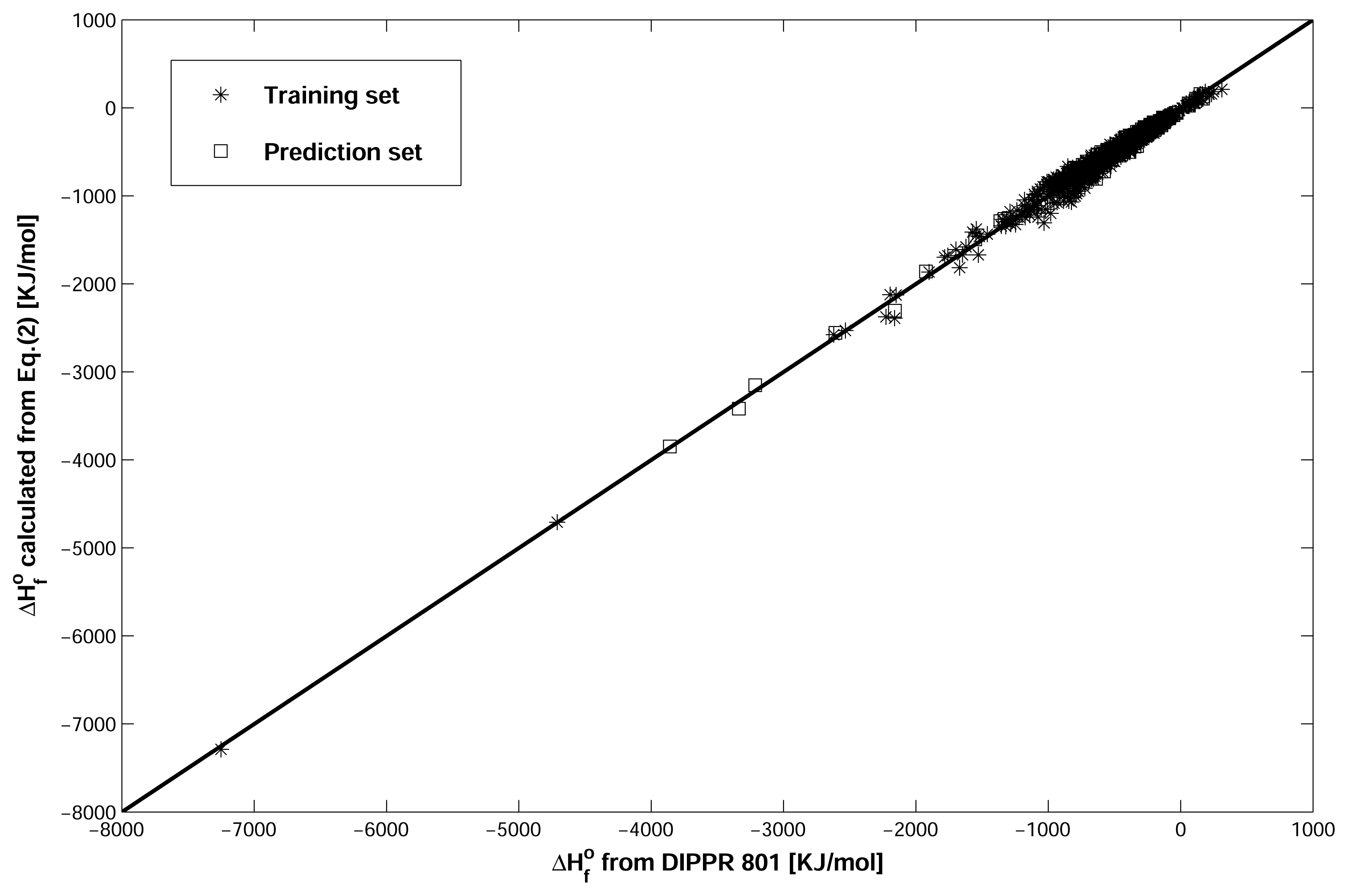
2.4. Validation of Model
3. Discussion
4. Conclusions


| Variable | Molecular descriptor meaning |
|---|---|
| nSK | Number of non-H atoms |
| SCBO | Sum of conventional bond orders (H-depleted) |
| nO | Number of Oxygen atoms |
| nF | Number of Fluorine atoms |
| nHM | Number of Heavy atoms |
| ID | Variable | Regression Coefficient | Errors Regression Coefficient | Confidence Intervals (0.95) | Standard Regression Coefficient |
|---|---|---|---|---|---|
| 0 | intercept | 50.16088267 | 4.075696 | 0 | 0 |
| 1 | nSK | −80.52012489 | 1.175295 | −1.081325919 | 3.60196 |
| 2 | SCBO | 53.64545627 | 0.9837223 | 0.858696667 | 3.593514 |
| 3 | nO | −169.2188895 | 1.424115 | −0.552855974 | 1.061814 |
| 4 | nF | −174.7547718 | 1.178939 | −0.680669749 | 1.047946 |
| 5 | nHM | −266.5765885 | 6.857063 | −0.171389892 | 1.006101 |
| ID | Name | ΔHf° (kJ/mol) | Res | |
|---|---|---|---|---|
| DIPPR 801 | Calculated from Eq. (2) | |||
| 1 | n-BUTANE | −125.79 | −110.98 | 14.81 |
| 2 | n-HEXANE | −198.66 | −164.73 | 33.93 |
| 3 | 3-METHYLPENTANE | −202.38 | −164.73 | 37.65 |
| 4 | n-HEPTANE | −224.05 | −191.61 | 32.44 |
| 5 | 3-METHYLHEXANE | −226.44 | −191.61 | 34.83 |
| 6 | 3-ETHYLPENTANE | −224.56 | −191.61 | 32.95 |
| 7 | 2,2-DIMETHYLPENTANE | −238.28 | −191.61 | 46.67 |
| 8 | 2,3-DIMETHYLPENTANE | −233.09 | −191.61 | 41.48 |
| 9 | 2,4-DIMETHYLPENTANE | −234.6 | −191.61 | 42.99 |
| 10 | 3,3-DIMETHYLPENTANE | −234.18 | −191.61 | 42.57 |
| 11 | 2,2,3-TRIMETHYLBUTANE | −236.52 | −191.61 | 44.91 |
| 12 | 2-METHYLHEPTANE | −255.01 | −218.48 | 36.53 |
| 13 | 4-METHYLHEPTANE | −251.63 | −218.48 | 33.15 |
| 14 | 3-ETHYLHEXANE | −250.41 | −218.48 | 31.93 |
| 15 | 2,2-DIMETHYLHEXANE | −261.88 | −218.48 | 43.4 |
| 16 | 2,3-DIMETHYLHEXANE | −252.59 | −218.48 | 34.11 |
| 17 | 2,4-DIMETHYLHEXANE | −257.02 | −218.48 | 38.54 |
| 18 | 3,3-DIMETHYLHEXANE | −257.53 | −218.48 | 39.05 |
| 19 | 2-METHYL-3-ETHYLPENTANE | −249.58 | −218.48 | 31.1 |
| 20 | 2,2,3-TRIMETHYLPENTANE | −256.9 | −218.48 | 38.42 |
| 21 | 2,2,4-TRIMETHYLPENTANE | −259.16 | −218.48 | 40.68 |
| 22 | 2,3,3-TRIMETHYLPENTANE | −253.51 | −218.48 | 35.03 |
| 23 | 2,3,4-TRIMETHYLPENTANE | −255.01 | −218.48 | 36.53 |
| 24 | n-NONANE | −274.68 | −245.36 | 29.32 |
| 25 | 3,3,5-TRIMETHYLHEPTANE | −304.76 | −272.23 | 32.53 |
| 26 | 2,4,4-TRIMETHYLHEXANE | −280.2 | −245.36 | 34.84 |
| 27 | 3,3-DIETHYLPENTANE | −275.39 | −245.36 | 30.03 |
| 28 | 2,2,3,3-TETRAMETHYLPENTANE | −278.28 | −245.36 | 32.92 |
| 29 | 2,2,4,4-TETRAMETHYLPENTANE | −279.99 | −245.36 | 34.63 |
| 30 | SQUALANE | −806.3 | −809.72 | −3.42 |
| 31 | n-DECANE | −300.62 | −272.23 | 28.39 |
| 32 | 2,2,5,5-TETRAMETHYLHEXANE | −323.51 | −272.23 | 51.28 |
| 33 | n-UNDECANE | −326.6 | −299.11 | 27.49 |
| 34 | n-DODECANE | −352.13 | −325.98 | 26.15 |
| 35 | n-TRIDECANE | −377.69 | −352.86 | 24.83 |
| 36 | n-TETRADECANE | −403.25 | −379.73 | 23.52 |
| 37 | n-PENTADECANE | −428.82 | −406.6 | 22.22 |
| 38 | n-HEXADECANE | −456.14 | −433.48 | 22.66 |
| 39 | n-OCTADECANE | −567.14 | −487.23 | 79.91 |
| 40 | n-NONADECANE | −596.21 | −514.1 | 82.11 |
| 41 | n-HENEICOSANE | −653.45 | −567.85 | 85.6 |
| 42 | n-DOCOSANE | −682.07 | −594.73 | 87.34 |
| 43 | n-TRICOSANE | −710.69 | −621.6 | 89.09 |
| 44 | n-PENTACOSANE | −767.93 | −675.35 | 92.58 |
| 45 | n-HEXACOSANE | −796.55 | −702.23 | 94.32 |
| 46 | n-HEPTACOSANE | −825.17 | −729.1 | 96.07 |
| 47 | n-OCTACOSANE | −853.79 | −755.98 | 97.81 |
| 48 | n-NONACOSANE | −882.41 | −782.85 | 99.56 |
| 49 | 2-METHYLNONANE | −311.9 | −272.23 | 39.67 |
| 50 | 5-METHYLNONANE | −310 | −272.23 | 37.77 |
| 51 | 2,2,4,4,6,8,8-HEPTAMETHYLNONANE | −476.87 | −433.48 | 43.39 |
| 52 | 3-METHYLOCTANE | −278.53 | −245.36 | 33.17 |
| 53 | 4-METHYLOCTANE | −279.6 | −245.36 | 34.24 |
| 54 | 3-ETHYLHEPTANE | −275.48 | −245.36 | 30.12 |
| 55 | 2,2-DIMETHYLHEPTANE | −288.2 | −245.36 | 42.84 |
| 56 | 3-METHYLUNDECANE | −355.2 | −325.98 | 29.22 |
| 57 | ETHYLCYCLOPENTANE | −163.43 | −137.96 | 25.47 |
| 58 | cis-1,2-DIMETHYLCYCLOPENTANE | −165.27 | −137.96 | 27.31 |
| 59 | trans-1,3-DIMETHYLCYCLOPENTANE | −168.07 | −137.96 | 30.11 |
| 60 | n-PROPYLCYCLOPENTANE | −189.07 | −164.84 | 24.23 |
| 61 | 1-METHYL-1-ETHYLCYCLOPENTANE | −193.8 | −164.84 | 28.96 |
| 62 | n-PROPYLCYCLOHEXANE | −237.4 | −191.71 | 45.69 |
| 63 | ISOPROPYLCYCLOHEXANE | −239.45 | −191.71 | 47.74 |
| 64 | 1,1-DIETHYLCYCLOHEXANE | −277.11 | −218.59 | 58.52 |
| 65 | n-DECYLCYCLOHEXANE | −417 | −379.83 | 37.17 |
| 66 | CYCLOHEPTANE | −156.61 | −137.96 | 18.65 |
| 67 | CYCLOOCTANE | −167.74 | −164.84 | 2.9 |
| 68 | trans-1,4-DIETHYLCYCLOHEXANE | −266.1 | −218.59 | 47.51 |
| 69 | 2,6-DIMETHYLHEPTANE | −286.12 | −245.36 | 40.76 |
| 70 | 2,2-DIMETHYL-3-ETHYLPENTANE | −272.7 | −245.36 | 27.34 |
| 71 | 2,4-DIMETHYL-3-ETHYLPENTANE | −269.7 | −245.36 | 24.34 |
| 72 | 1-TRIACONTENE | −761.6 | −756.08 | 5.52 |
| 73 | 2-METHYL-1-BUTENE | −60.96 | −84.21 | −23.25 |
| 74 | cis-2-HEXENE | −80.11 | −111.09 | −30.98 |
| 75 | trans-2-HEXENE | −85.52 | −111.09 | −25.57 |
| 76 | cis-3-HEXENE | −78.95 | −111.09 | −32.14 |
| 77 | 2-METHYL-1-PENTENE | −89.96 | −111.09 | −21.13 |
| 78 | 3-METHYL-1-PENTENE | −78.16 | −111.09 | −32.93 |
| 79 | 4-METHYL-1-PENTENE | −80.04 | −111.09 | −31.05 |
| 80 | 2-METHYL-2-PENTENE | −98.53 | −111.09 | −12.56 |
| 81 | 4-METHYL-1-HEXENE | −101.5 | −137.96 | −36.46 |
| 82 | 4-METHYL-cis-2-PENTENE | −87.03 | −111.09 | −24.06 |
| 83 | 4-METHYL-trans-2-PENTENE | −91.55 | −111.09 | −19.54 |
| 84 | 2-ETHYL-1-BUTENE | −87.11 | −111.09 | −23.98 |
| 85 | 2,3-DIMETHYL-1-BUTENE | −95.6 | −111.09 | −15.49 |
| 86 | 3,3-DIMETHYL-1-BUTENE | −88.28 | −111.09 | −22.81 |
| 87 | 2-ETHYL-1-PENTENE | −109.9 | −137.96 | −28.06 |
| 88 | 1-HEPTENE | −98.37 | −137.96 | −39.59 |
| 89 | cis-2-HEPTENE | −105.1 | −137.96 | −32.86 |
| 90 | trans-2-HEPTENE | −109.5 | −137.96 | −28.46 |
| 91 | trans-3-HEPTENE | −109.33 | −137.96 | −28.63 |
| 92 | 2-METHYL-1-HEXENE | −112.6 | −137.96 | −25.36 |
| 93 | 3-ETHYL-1-PENTENE | −98.49 | −137.96 | −39.47 |
| 94 | 3-METHYL-1-HEXENE | −101.1 | −137.96 | −36.86 |
| 95 | 3-ETHYL-1-HEXENE | −124.6 | −164.84 | −40.24 |
| 96 | 2,3,3-TRIMETHYL-1-BUTENE | −117.7 | −137.96 | −20.26 |
| 97 | cis-3-HEPTENE | −104.35 | −137.96 | −33.61 |
| 98 | 1-OCTENE | −122 | −164.84 | −42.84 |
| 99 | 2,4,4-TRIMETHYL-1-PENTENE | −146.15 | −164.84 | −18.69 |
| 100 | 2-ETHYL-1-HEXENE | −136.42 | −164.84 | −28.42 |
| 101 | 1-NONENE | −148.8 | −191.71 | −42.91 |
| 102 | 1-UNDECENE | −200.8 | −245.46 | −44.66 |
| 103 | 1-DODECENE | −226.2 | −272.34 | −46.14 |
| 104 | 1-TRIDECENE | −253.5 | −299.21 | −45.71 |
| 105 | 1-TETRADECENE | −280.3 | −326.08 | −45.78 |
| 106 | 1-HEXADECENE | −329.24 | −379.83 | −50.59 |
| 107 | 1-OCTADECENE | −374.77 | −433.58 | −58.81 |
| 108 | 6-METHYL-1-HEPTENE | −129.5 | −164.84 | −35.34 |
| 109 | CYCLOHEXENE | −38.2 | −57.44 | −19.24 |
| 110 | trans-2-EICOSENE | −446.6 | −487.33 | −40.73 |
| 111 | trans-2-PENTADECENE | −319.5 | −352.96 | −33.46 |
| 112 | cis-2-OCTENE | −129.4 | −164.84 | −35.44 |
| 113 | trans-3-OCTENE | −134.38 | −164.84 | −30.46 |
| 114 | cis-4-OCTENE | −128.49 | −164.84 | −36.35 |
| 115 | trans-4-OCTENE | −134.61 | −164.84 | −30.23 |
| 116 | cis-3-OCTENE | −129.14 | −164.84 | −35.7 |
| 117 | 1-EICOSENE | −459.21 | −487.33 | −28.12 |
| 118 | 1-METHYLCYCLOPENTENE | −36.44 | −57.44 | −21 |
| 119 | 2,3-DIMETHYL-1-HEXENE | −136 | −164.84 | −28.84 |
| 120 | 1,4-DI-tert-BUTYLBENZENE | −188.9 | −165.15 | 23.75 |
| 121 | alpha-TOCOPHEROL | −873.4 | −879.94 | −6.54 |
| 122 | 1,2,3-TRIETHYLBENZENE | −130.32 | −111.4 | 18.92 |
| 123 | n-HEPTYLBENZENE | −140.6 | −138.27 | 2.33 |
| 124 | 1,2,3,5-TETRAETHYLBENZENE | −196.36 | −165.15 | 31.21 |
| 125 | n-DECYLBENZENE | −217.5 | −218.9 | −1.4 |
| 126 | PENTAETHYLBENZENE | −258.1 | −218.9 | 39.2 |
| 127 | m-TERPHENYL | 165.58 | 156.52 | −9.06 |
| 128 | n-PENTYLBENZENE | −89.5 | −84.52 | 4.98 |
| 129 | n-HEXYLBENZENE | −115 | −111.4 | 3.6 |
| 130 | n-OCTYLBENZENE | −166.1 | −165.15 | 0.95 |
| 131 | n-NONYLBENZENE | −190.4 | −192.02 | −1.62 |
| 132 | n-UNDECYLBENZENE | −241.18 | −245.77 | −4.59 |
| 133 | n-TRIDECYLBENZENE | −288.73 | −299.52 | −10.79 |
| 134 | n-TETRADECYLBENZENE | −311.49 | −326.4 | −14.91 |
| 135 | n-DODECYLBENZENE | −264.79 | −272.65 | −7.86 |
| 136 | 2,3-DIMETHYL-2,3-DIPHENYLBUTANE | −59.68 | −58.06 | 1.62 |
| 137 | 1,1,2-TRIPHENYLETHANE | 130.2 | 102.77 | −27.43 |
| 138 | TETRAPHENYLMETHANE | 247.1 | 182.98 | −64.12 |
| 139 | 1,1,2,2-TETRAPHENYLETHANE | 216 | 156.1 | −59.9 |
| 140 | 1-(4-ETHYLPHENYL)-2-PHENYLETHANE | 12.03 | −4.32 | −16.35 |
| 141 | STYRENE | 103.47 | 49.75 | −53.72 |
| 142 | 1-n-NONYLNAPHTHALENE | −132.57 | −111.76 | 20.81 |
| 143 | 1-n-DECYLNAPHTHALENE | −156.26 | −138.64 | 17.62 |
| 144 | 1-n-HEXYL-1,2,3,4-TETRAHYDRONAPHTHALENE | −179.33 | −165.25 | 14.08 |
| 145 | 1-PHENYLINDENE | 148.61 | 129.85 | −18.76 |
| 146 | TRIPHENYLETHYLENE | 233.38 | 156.41 | −76.97 |
| 147 | TETRAPHENYLETHYLENE | 311.5 | 209.75 | −101.75 |
| 148 | trans-STILBENE | 136.9 | 103.08 | −33.82 |
| 149 | ACENAPHTHALENE | 186.6 | 183.65 | −2.95 |
| 150 | sec-BUTYLCYCLOHEXANE | −263.7 | −218.59 | 45.11 |
| 151 | PIMARIC ACID | −634.1 | −611.29 | 22.81 |
| 152 | ISOPIMARIC ACID | −670.4 | −611.29 | 59.11 |
| 153 | SULFUR DIOXIDE | −296.84 | −315.26 | −18.42 |
| 154 | SULFUR TRIOXIDE | −441.04 | −457.7 | −16.66 |
| 155 | ACETALDEHYDE | −166.4 | −199.68 | −33.28 |
| 156 | PROPANAL | −215.3 | −226.56 | −11.26 |
| 157 | 1,2,3,6-TETRAHYDROBENZALDEHYDE | −162.1 | −226.76 | −64.66 |
| 158 | BUTANAL | −239.2 | −253.43 | −14.23 |
| 159 | HEPTANAL | −311.5 | −334.06 | −22.56 |
| 160 | HEXANAL | −291.83 | −307.18 | −15.35 |
| 161 | OCTANAL | −342.7 | −360.93 | −18.23 |
| 162 | NONANAL | −367.93 | −387.8 | −19.87 |
| 163 | 2-ETHYLHEXANAL | −348.5 | −360.93 | −12.43 |
| 164 | 2-METHYLHEXANAL | −317.47 | −334.06 | −16.59 |
| 165 | 2-METHYL-2-PENTENAL | −201.8 | −253.54 | −51.74 |
| 166 | 2-ETHYL-2-HEXENAL | −244.6 | −307.28 | −62.68 |
| 167 | DECANAL | −393.84 | −414.68 | −20.84 |
| 168 | UNDECANAL | −419.06 | −441.55 | −22.49 |
| 169 | DODECANAL | −445.25 | −468.43 | −23.18 |
| 170 | 2-METHYLBUTYRALDEHYDE | −271.5 | −280.31 | −8.81 |
| 171 | 3-METHYLBUTYRALDEHYDE | −276.5 | −280.31 | −3.81 |
| 172 | cis-CROTONALDEHYDE | −137.7 | −199.79 | −62.09 |
| 173 | trans-CROTONALDEHYDE | −138.7 | −199.79 | −61.09 |
| 174 | o-TOLUALDEHYDE | −113.18 | −146.35 | −33.17 |
| 175 | p-HYDROXYBENZALDEHYDE | −310.82 | −315.57 | −4.75 |
| 176 | TEREPHTHALDEHYDE | −243.43 | −288.8 | −45.37 |
| 177 | 2-METHYL OCTANAL | −370.2 | −387.8 | −17.6 |
| 178 | METHYL ETHYL KETONE | −273.3 | −253.43 | 19.87 |
| 179 | METHYL ISOBUTYL KETONE | −328.4 | −307.18 | 21.22 |
| 180 | 3-METHYL-2-PENTANONE | −323.8 | −307.18 | 16.62 |
| 181 | 3-HEPTANONE | −348.6 | −334.06 | 14.54 |
| 182 | 4-HEPTANONE | −346.2 | −334.06 | 12.14 |
| 183 | 3-HEXANONE | −320.2 | −307.18 | 13.02 |
| 184 | 2-HEXANONE | −322.01 | −307.18 | 14.83 |
| 185 | MESITYL OXIDE | −238.14 | −253.54 | −15.4 |
| 186 | 3,3-DIMETHYL-2-BUTANONE | −328.6 | −307.18 | 21.42 |
| 187 | DIISOBUTYL KETONE | −408.5 | −387.8 | 20.7 |
| 188 | DIISOPROPYL KETONE | −352.92 | −334.06 | 18.86 |
| 189 | 2-PYRROLIDONE | −266.04 | −226.66 | 39.38 |
| 190 | N-METHYL-2-PYRROLIDONE | −262.2 | −253.54 | 8.66 |
| 191 | ETHYL ISOAMYL KETONE | −374.4 | −360.93 | 13.47 |
| 192 | 5-NONANONE | −398.24 | −387.8 | 10.44 |
| 193 | 2-NONANONE | −396.8 | −387.8 | 9 |
| 194 | ACETYLACETONE | −423.8 | −422.75 | 1.05 |
| 195 | CYCLOPENTANONE | −235.7 | −226.66 | 9.04 |
| 196 | CYCLOHEXANONE | −271.2 | −253.54 | 17.66 |
| 197 | 2-OCTANONE | −372.7 | −360.93 | 11.77 |
| 198 | BENZOPHENONE | −37.3 | −66.14 | −28.84 |
| 199 | ACETOPHENONE | −142.5 | −146.35 | −3.85 |
| 200 | beta-PROPIOLACTONE | −329.9 | −369 | −39.1 |
| 201 | 2-CYCLOHEXYL CYCLOHEXANONE | −390.98 | −361.14 | 29.84 |
| 202 | METHANOL | −239.1 | −226.45 | 12.65 |
| 203 | ETHANOL | −276.98 | −253.33 | 23.65 |
| 204 | 1-PROPANOL | −302.6 | −280.2 | 22.4 |
| 205 | ISOPROPANOL | −318.1 | −280.2 | 37.9 |
| 206 | 1-BUTANOL | −327.2 | −307.08 | 20.12 |
| 207 | 2-BUTANOL | −342.6 | −307.08 | 35.52 |
| 208 | 2-METHYL-2-PROPANOL | −365.9 | −307.08 | 58.82 |
| 209 | 1-PENTANOL | −351.6 | −333.95 | 17.65 |
| 210 | 2-PENTANOL | −365.2 | −333.95 | 31.25 |
| 211 | 2-METHYL-1-BUTANOL | −356.6 | −333.95 | 22.65 |
| 212 | 2,2-DIMETHYL-1-PROPANOL | −382.01 | −333.95 | 48.06 |
| 213 | 1-HEXANOL | −377.5 | −360.83 | 16.67 |
| 214 | 2-HEXANOL | −392 | −360.83 | 31.17 |
| 215 | 3-METHYL-1-PENTANOL | −380.9 | −360.83 | 20.07 |
| 216 | 3-PENTANOL | −370.33 | −333.95 | 36.38 |
| 217 | 2-ETHYL-1-HEXANOL | −432.8 | −414.58 | 18.22 |
| 218 | 2-METHYL-1-HEXANOL | −404.5 | −387.7 | 16.8 |
| 219 | 3-METHYL-1-BUTANOL | −356.4 | −333.95 | 22.45 |
| 220 | 1-HEPTANOL | −403.3 | −387.7 | 15.6 |
| 221 | 1-NONANOL | −453.6 | −441.45 | 12.15 |
| 222 | 1-DECANOL | −478.1 | −468.32 | 9.78 |
| 223 | 1-UNDECANOL | −504.8 | −495.2 | 9.6 |
| 224 | 8-METHYL-1-NONANOL | −483.13 | −468.32 | 14.81 |
| 225 | 1-DODECANOL | −528.5 | −522.07 | 6.43 |
| 226 | 1-TRIDECANOL | −599.4 | −548.95 | 50.45 |
| 227 | 1-TETRADECANOL | −628.18 | −575.82 | 52.36 |
| 228 | 1-PENTADECANOL | −658.2 | −602.7 | 55.5 |
| 229 | 1-HEPTADECANOL | −722.85 | −656.45 | 66.4 |
| 230 | 2-ETHYL-1-BUTANOL | −382.41 | −360.83 | 21.58 |
| 231 | 1-METHYLCYCLOHEXANOL | −388.17 | −334.06 | 54.11 |
| 232 | cis-2-METHYLCYCLOHEXANOL | −390.2 | −334.06 | 56.14 |
| 233 | cis-3-METHYLCYCLOHEXANOL | −416.1 | −334.06 | 82.04 |
| 234 | trans-3-METHYLCYCLOHEXANOL | −394.4 | −334.06 | 60.34 |
| 235 | cis-4-METHYLCYCLOHEXANOL | −413.2 | −334.06 | 79.14 |
| 236 | trans-4-METHYLCYCLOHEXANOL | −433.3 | −334.06 | 99.24 |
| 237 | AGATHADIOL | −685.7 | −718.58 | −32.88 |
| 238 | alpha-TERPINEOL | −316.7 | −361.03 | −44.33 |
| 239 | 2-BUTYL-NONAN-1-OL | −540.1 | −548.95 | −8.85 |
| 240 | TETRAHYDROFURFURYL ALCOHOL | −435.7 | −476.4 | −40.7 |
| 241 | 2-PHENYL-2-PROPANOL | −244.43 | −226.87 | 17.56 |
| 242 | 2-BUTYL-OCTAN-1-OL | −512.2 | −522.07 | −9.87 |
| 243 | 2,6-XYLENOL | −237.4 | −199.99 | 37.41 |
| 244 | BENZYL ALCOHOL | −160.71 | −173.12 | −12.41 |
| 245 | m-CRESOL | −194 | −173.12 | 20.88 |
| 246 | o-ETHYLPHENOL | −208.82 | −199.99 | 8.83 |
| 247 | p-HYDROQUINONE | −371.1 | −342.34 | 28.76 |
| 248 | p-ETHYLPHENOL | −224.39 | −199.99 | 24.4 |
| 249 | p-tert-BUTYLPHENOL | −276.66 | −253.74 | 22.92 |
| 250 | BISPHENOL A | −368.5 | −369.63 | −1.13 |
| 251 | NONYLPHENOL | −387.33 | −388.12 | −0.79 |
| 252 | ETHYLENE GLYCOL | −460 | −449.42 | 10.58 |
| 253 | DIETHYLENE GLYCOL | −628.5 | −699.26 | −70.76 |
| 254 | TETRAETHYLENE GLYCOL | −981.7 | −1198.95 | −217.25 |
| 255 | 1,2-PROPYLENE GLYCOL | −499.99 | −476.3 | 23.69 |
| 256 | 1,3-PROPYLENE GLYCOL | −480.8 | −476.3 | 4.5 |
| 257 | DIPROPYLENE GLYCOL | −718.46 | −753.01 | −34.55 |
| 258 | 2-METHYL-1,3-PROPANEDIOL | −505.9 | −503.17 | 2.73 |
| 259 | 1,2-BUTANEDIOL | −523.6 | −503.17 | 20.43 |
| 260 | 1,3-BUTANEDIOL | −501 | −503.17 | −2.17 |
| 261 | HEXYLENE GLYCOL | −602.92 | −556.92 | 46 |
| 262 | GLYCEROL | −669.6 | −672.39 | −2.79 |
| 263 | p-tert-BUTYLCATECHOL | −474 | −449.84 | 24.16 |
| 264 | 2,2,4-TRIMETHYL-1,3-PENTANEDIOL | −497.18 | −610.67 | −113.49 |
| 265 | 2-METHYL-1,3-PENTANEDIOL | −577.5 | −556.92 | 20.58 |
| 266 | 2,3-BUTANEDIOL | −541.5 | −503.17 | 38.33 |
| 267 | cis-2-BUTENE-1,4-DIOL | −372.9 | −449.52 | −76.62 |
| 268 | trans-2-BUTENE-1,4-DIOL | −401.6 | −449.52 | −47.92 |
| 269 | 1,5-PENTANEDIOL | −531.49 | −530.05 | 1.44 |
| 270 | 1,6-HEXANEDIOL | −583.86 | −556.92 | 26.94 |
| 271 | 1,2-BENZENEDIOL | −354.1 | −342.34 | 11.76 |
| 272 | 1,3-BENZENEDIOL | −368 | −342.34 | 25.66 |
| 273 | PENTAERYTHRITOL | −920.6 | −922.23 | −1.63 |
| 274 | TRIMETHYLOLPROPANE | −751.61 | −753.01 | −1.4 |
| 275 | 1,2,3-BENZENETRIOL | −551.1 | −538.43 | 12.67 |
| 276 | SORBITOL | −1354.2 | −1341.29 | 12.91 |
| 277 | FORMIC ACID | −425.5 | −368.9 | 56.6 |
| 278 | ACETIC ACID | −484.5 | −395.78 | 88.72 |
| 279 | PROPIONIC ACID | −508.5 | −422.65 | 85.85 |
| 280 | n-DECANOIC ACID | −713.7 | −610.77 | 102.93 |
| 281 | OXALIC ACID | −829.7 | −734.32 | 95.38 |
| 282 | n-BUTYRIC ACID | −533.8 | −449.52 | 84.28 |
| 283 | n-PENTANOIC ACID | −558.7 | −476.4 | 82.3 |
| 284 | n-NONANOIC ACID | −661.8 | −583.9 | 77.9 |
| 285 | ISOBUTYRIC ACID | −531 | −449.52 | 81.48 |
| 286 | ISOVALERIC ACID | −561.6 | −476.4 | 85.2 |
| 287 | n-HEXANOIC ACID | −583.8 | −503.27 | 80.53 |
| 288 | 2-METHYLHEXANOIC ACID | −613.9 | −530.15 | 83.75 |
| 289 | 1,4-CYCLOHEXANEDICARBOXYLIC ACID | −998.5 | −841.92 | 156.58 |
| 290 | n-OCTANOIC ACID | −636.8 | −557.02 | 79.78 |
| 291 | n-UNDECANOIC ACID | −735.9 | −637.65 | 98.25 |
| 292 | CYCLOPENTYLACETIC ACID | −551.73 | −476.5 | 75.23 |
| 293 | DILACTIC ACID | −1122.8 | −1037.91 | 84.89 |
| 294 | n-DODECANOIC ACID | −774.6 | −664.52 | 110.08 |
| 295 | n-HEXADECANOIC ACID | −891.5 | −772.02 | 119.48 |
| 296 | trans-CROTONIC ACID | −446.23 | −395.88 | 50.35 |
| 297 | STEARIC ACID | −948 | −825.77 | 122.23 |
| 298 | ACRYLIC ACID | −383.88 | −369 | 14.88 |
| 299 | OLEIC ACID | −802.49 | −772.12 | 30.37 |
| 300 | LINOLEIC ACID | −674.04 | −718.48 | −44.44 |
| 301 | SALICYLIC ACID | −589.9 | −511.66 | 78.24 |
| 302 | ADIPIC ACID | −994.3 | −841.82 | 152.48 |
| 303 | MALEIC ACID | −789.4 | −734.42 | 54.98 |
| 304 | TEREPHTHALIC ACID | −816.18 | −680.98 | 135.2 |
| 305 | ACETIC ANHYDRIDE | −624.4 | −591.97 | 32.43 |
| 306 | PROPIONIC ANHYDRIDE | −679.1 | −645.72 | 33.38 |
| 307 | BUTYRIC ANHYDRIDE | −719.12 | −699.47 | 19.65 |
| 308 | PALUSTRIC ACID | −852.4 | −664.94 | 187.46 |
| 309 | SUCCINIC ANHYDRIDE | −607.8 | −538.33 | 69.47 |
| 310 | GLUTARIC ANHYDRIDE | −618.5 | −565.2 | 53.3 |
| 311 | PHTHALIC ANHYDRIDE | −460.1 | −431.24 | 28.86 |
| 312 | MALEIC ANHYDRIDE | −469.8 | −484.68 | −14.88 |
| 313 | TRIMELLITIC ANHYDRIDE | −894.81 | −796.66 | 98.15 |
| 314 | METHYL FORMATE | −386.1 | −395.78 | −9.68 |
| 315 | n-PROPYL FORMATE | −445.2 | −449.52 | −4.32 |
| 316 | n-BUTYL FORMATE | −469.2 | −476.4 | −7.2 |
| 317 | ISOBUTYL FORMATE | −475.87 | −476.4 | −0.53 |
| 318 | n-PENTYL FORMATE | −493.28 | −503.27 | −9.99 |
| 319 | n-OCTYL FORMATE | −566.45 | −583.9 | −17.45 |
| 320 | n-NONYL FORMATE | −588.93 | −610.77 | −21.84 |
| 321 | n-DECYL FORMATE | −613.73 | −637.65 | −23.92 |
| 322 | VINYL FORMATE | −293.36 | −369 | −75.64 |
| 323 | ETHYL ACETATE | −478.8 | −449.52 | 29.28 |
| 324 | n-PROPYL ACETATE | −504.32 | −476.4 | 27.92 |
| 325 | n-BUTYL ACETATE | −529.2 | −503.27 | 25.93 |
| 326 | ISOBUTYL ACETATE | −536.06 | −503.27 | 32.79 |
| 327 | ISOPENTYL ACETATE | −558.69 | −530.15 | 28.54 |
| 328 | ALLYL ACETATE | −386.3 | −422.75 | −36.45 |
| 329 | ISOPROPYL ACETATE | −518.8 | −476.4 | 42.4 |
| 330 | sec-BUTYL ACETATE | −544.04 | −503.27 | 40.77 |
| 331 | VINYL ACETATE | −349.7 | −395.88 | −46.18 |
| 332 | METHYL PROPIONATE | −463.3 | −449.52 | 13.78 |
| 333 | ETHYL PROPIONATE | −502.7 | −476.4 | 26.3 |
| 334 | n-PROPYL PROPIONATE | −527.5 | −503.27 | 24.23 |
| 335 | n-BUTYL PROPIONATE | −549.9 | −530.15 | 19.75 |
| 336 | VINYL PROPIONATE | −385.46 | −422.75 | −37.29 |
| 337 | ETHYL n-BUTYRATE | −514.63 | −503.27 | 11.36 |
| 338 | n-PROPYL ISOBUTYRATE | −564.5 | −530.15 | 34.35 |
| 339 | METHYL ACRYLATE | −362.2 | −395.88 | −33.68 |
| 340 | ETHYL ACRYLATE | −379.59 | −422.75 | −43.16 |
| 341 | n-PROPYL ACRYLATE | −407.17 | −449.63 | −42.46 |
| 342 | n-BUTYL NONANOATE | −697.78 | −691.4 | 6.38 |
| 343 | n-BUTYL VALERATE | −613.3 | −583.9 | 29.4 |
| 344 | ETHYL ISOVALERATE | −570.9 | −530.15 | 40.75 |
| 345 | METHYL METHACRYLATE | −399.13 | −422.75 | −23.62 |
| 346 | ETHYL METHACRYLATE | −421.34 | −449.63 | −28.29 |
| 347 | n-PROPYL METHACRYLATE | −446.7 | −476.5 | −29.8 |
| 348 | DIOCTYL PHTHALATE | −1084.1 | −1110.98 | −26.88 |
| 349 | DIISOOCTYL PHTHALATE | −1087.3 | −1110.98 | −23.68 |
| 350 | 1,2-BENZENEDICARBOXYLIC ACID, HEPTYL, NONYL ESTER | −1085 | −1110.98 | −25.98 |
| 351 | n-PENTYL ACETATE | −553 | −530.15 | 22.85 |
| 352 | 2-ETHYLHEXYL ACETATE | −627.99 | −610.77 | 17.22 |
| 353 | BENZYL ACETATE | −368.8 | −369.32 | −0.52 |
| 354 | ISOBUTYL ISOBUTYRATE | −594.07 | −557.02 | 37.05 |
| 355 | ISOPENTYL ISOVALERATE | −644.74 | −610.77 | 33.97 |
| 356 | METHYL OLEATE | −734.5 | −799 | −64.5 |
| 357 | n-HEXYL ACETATE | −577.9 | −557.02 | 20.88 |
| 358 | n-BUTYL BENZOATE | −429.06 | −423.07 | 5.99 |
| 359 | n-HEPTYL ACETATE | −602.67 | −583.9 | 18.77 |
| 360 | n-OCTYL ACETATE | −628.25 | −610.77 | 17.48 |
| 361 | n-DECYL ACETATE | −679.25 | −664.52 | 14.73 |
| 362 | DIISODECYL PHTHALATE | −1196.9 | −1218.48 | −21.58 |
| 363 | METHYL SALICYLATE | −531.79 | −538.54 | −6.75 |
| 364 | DI-n-NONYL PHTHALATE | −1134.8 | −1164.73 | −29.93 |
| 365 | DI-n-PROPYL PHTHALATE | −811.89 | −842.23 | −30.34 |
| 366 | DIISOBUTYL PHTHALATE | −890 | −895.98 | −5.98 |
| 367 | DIMETHYL ISOPHTHALATE | −730.9 | −734.73 | −3.83 |
| 368 | DI-n-DECYL PHTHALATE | −1197 | −1218.48 | −21.48 |
| 369 | DI-n-UNDECYL PHTHALATE | −1248 | −1325.98 | −77.98 |
| 370 | DI-n-HEXYL PHTHALATE | −987.8 | −1003.48 | −15.68 |
| 371 | DIMETHYL TEREPHTHALATE | −732.6 | −734.73 | −2.13 |
| 372 | DI-n-OCTYL TEREPHTHALATE | −1181.2 | −1110.98 | 70.22 |
| 373 | n-BUTYL STEARATE | −978.16 | −933.27 | 44.89 |
| 374 | DIBUTYL SEBACATE | −1156.7 | −1164.31 | −7.61 |
| 375 | n-BUTYL n-BUTYRATE | −575.39 | −557.02 | 18.37 |
| 376 | n-BUTYL METHACRYLATE | −471.39 | −503.38 | −31.99 |
| 377 | METHYL BENZOATE | −343.5 | −342.44 | 1.06 |
| 378 | ETHYL BENZOATE | −379.91 | −369.32 | 10.59 |
| 379 | DIETHYL CARBONATE | −682.65 | −672.49 | 10.16 |
| 380 | DIETHYL OXALATE | −806.28 | −841.82 | −35.54 |
| 381 | DIETHYL MALONATE | −838.02 | −868.69 | −30.67 |
| 382 | ISOPROPYL MYRISTATE | −820.33 | −798.9 | 21.43 |
| 383 | TRI-n-HEPTYL TRIMELLITATE | −1697 | −1610.77 | 86.23 |
| 384 | 1,2-BENZENE DICARBOXYLIC ACID, HEPTYL, UNDECYL ESTER | −1137 | −1164.73 | −27.73 |
| 385 | DIMETHYL ETHER | −184.1 | −253.33 | −69.23 |
| 386 | DIETHYL ETHER | −279.4 | −307.08 | −27.68 |
| 387 | DIISOPROPYL ETHER | −351.5 | −360.83 | −9.33 |
| 388 | DI-n-BUTYL ETHER | −377.9 | −414.58 | −36.68 |
| 389 | METHYL tert-BUTYL ETHER | −313.6 | −333.95 | −20.35 |
| 390 | DI-sec-BUTYL ETHER | −401.5 | −414.58 | −13.08 |
| 391 | METHYL ETHYL ETHER | −216.4 | −280.2 | −63.8 |
| 392 | METHYL n-PROPYL ETHER | −265.89 | −307.08 | −41.19 |
| 393 | ISOPROPYL BUTYL ETHER | −365.64 | −387.7 | −22.06 |
| 394 | METHYL ISOBUTYL ETHER | −296.13 | −333.95 | −37.82 |
| 395 | DI-n-HEXYL ETHER | −481.96 | −522.07 | −40.11 |
| 396 | METHYL n-BUTYL ETHER | −290.6 | −333.95 | −43.35 |
| 397 | ETHYL PROPYL ETHER | −303.59 | −333.95 | −30.36 |
| 398 | 1,4-DIOXANE | −355.1 | −449.52 | −94.42 |
| 399 | TRIOXANE | −522.5 | −618.74 | −96.24 |
| 400 | DI-tert-BUTYL ETHER | −399.61 | −414.58 | −14.97 |
| 401 | DI-n-OCTYL ETHER | −582.75 | −629.57 | −46.82 |
| 402 | DI-n-PENTYL ETHER | −425.12 | −468.32 | −43.2 |
| 403 | METHYL sec-BUTYL ETHER | −305.24 | −333.95 | −28.71 |
| 404 | tert-BUTYL ETHYL ETHER | −346.83 | −360.83 | −14 |
| 405 | METHYL n-PENTYL ETHER | −315.1 | −360.83 | −45.73 |
| 406 | ETHYL tert-PENTYL ETHER | −369.07 | −387.7 | −18.63 |
| 407 | METHYLAL | −378.2 | −476.3 | −98.1 |
| 408 | ACETAL | −491.41 | −556.92 | −65.51 |
| 409 | ETHYL ISOBUTYL ETHER | −333.5 | −360.83 | −27.33 |
| 410 | DI-n-PROPYL ETHER | −328.82 | −360.83 | −32.01 |
| 411 | n-BUTYL ETHYL ETHER | −328.7 | −360.83 | −32.13 |
| 412 | DIETHYLENE GLYCOL DI-n-BUTYL ETHER | −723.58 | −914.26 | −190.68 |
| 413 | BENZYL ETHYL ETHER | −165.78 | −226.87 | −61.09 |
| 414 | PHENETOLE | −152.6 | −199.99 | −47.39 |
| 415 | 1-METHYL-3-(METHYLETHOXY)BENZENE | −221.6 | −253.74 | −32.14 |
| 416 | 1,1-DIMETHOXYETHANE | −420.1 | −503.17 | −83.07 |
| 417 | 2,5-DIHYDROFURAN | −141.36 | −199.79 | −58.43 |
| 418 | TETRAHYDROFURAN | −216.19 | −253.43 | −37.24 |
| 419 | 1-tert-BUTOXY-2-[2-(tert-BUTOXY)PROPOXY]PROPANE | −810.3 | −968.01 | −157.71 |
| 420 | 1,2-DIMETHOXYPROPANE | −422.3 | −530.05 | −107.75 |
| 421 | sec-BUTYL-tert-BUTYL ETHER | −417.5 | −414.58 | 2.92 |
| 422 | ISOBUTYL-tert-BUTYL ETHER | −407 | −414.58 | −7.58 |
| 423 | 1,4-DICHLORO-trans-2-BUTENE | −112.53 | −111.09 | 1.44 |
| 424 | HEXACHLOROETHANE | −202.8 | −218.48 | −15.68 |
| 425 | 1,1,1,2-TETRACHLOROETHANE | −191 | −164.73 | 26.27 |
| 426 | 1,1,2,2-TETRACHLOROETHANE | −194.6 | −164.73 | 29.87 |
| 427 | HEXACHLOROCYCLOPENTADIENE | −159.78 | −138.17 | 21.61 |
| 428 | PENTACHLOROETHANE | −187.6 | −191.61 | −4.01 |
| 429 | 3,4-DICHLORO-1-BUTENE | −106.91 | −111.09 | −4.18 |
| 430 | DICHLORODIFLUOROMETHANE | −491.62 | −487.37 | 4.25 |
| 431 | TRICHLOROFLUOROMETHANE | −288.7 | −312.61 | −23.91 |
| 432 | CHLOROTRIFLUOROMETHANE | −707.93 | −662.12 | 45.81 |
| 433 | 2-CHLORO-1,1,1-TRIFLUOROETHANE | −741.8 | −689 | 52.8 |
| 434 | 1,2-DICHLOROTETRAFLUOROETHANE | −916.3 | −917.5 | −1.2 |
| 435 | 1,2-DIBROMOTETRAFLUOROETHANE | −807.1 | −917.5 | −110.4 |
| 436 | METHYL FLUORIDE | −234.3 | −231.99 | 2.31 |
| 437 | DIFLUOROMETHANE | −452.3 | −433.62 | 18.68 |
| 438 | TRIFLUOROMETHANE | −697.05 | −635.25 | 61.8 |
| 439 | CARBON TETRAFLUORIDE | −933.15 | −836.88 | 96.27 |
| 440 | ETHYL FLUORIDE | −264.4 | −258.86 | 5.54 |
| 441 | 1,1,1-TRIFLUOROETHANE | −736.4 | −662.12 | 74.28 |
| 442 | DECAFLUOROBUTANE | −2149.7 | −2127.28 | 22.42 |
| 443 | PERFLUORO-n-DECANE | −4710 | −4708.08 | 1.92 |
| 444 | 1,1-DIFLUOROETHYLENE | −328.96 | −406.85 | −77.89 |
| 445 | TETRAFLUOROETHYLENE | −658.56 | −810.11 | −151.55 |
| 446 | BROMODIFLUOROMETHANE | −424.9 | −460.49 | −35.59 |
| 447 | 1,1-DIFLUOROETHANE | −497 | −460.49 | 36.51 |
| 448 | 1-BROMOPROPANE | −121.8 | −110.98 | 10.82 |
| 449 | 1-BROMOBUTANE | −143.8 | −137.86 | 5.94 |
| 450 | 1-BROMOHEPTANE | −218.4 | −218.48 | −0.08 |
| 451 | 1,2-DIBROMOETHANE | −79.2 | −110.98 | −31.78 |
| 452 | 1,1,1-TRICHLOROTRIFLUOROETHANE | −822 | −742.75 | 79.25 |
| 453 | ISOPROPYL IODIDE | −74.8 | −110.98 | −36.18 |
| 454 | 2,2-DICHLORO-1,1,1-TRIFLUOROETHANE | −770.3 | −715.87 | 54.43 |
| 455 | HEXAFLUOROPROPYLENE | −1079 | −1240.24 | −161.24 |
| 456 | 2-METHYL-2-AMINOBUTANE | −171.4 | −164.73 | 6.67 |
| 457 | DI-n-PROPYLAMINE | −156.11 | −191.61 | −35.5 |
| 458 | DIETHYLAMINE | −103.7 | −137.86 | −34.16 |
| 459 | n-PROPYLAMINE | −101.47 | −110.98 | −9.51 |
| 460 | n-PENTYLAMINE | −152.62 | −164.73 | −12.11 |
| 461 | ISOBUTYLAMINE | −132.6 | −137.86 | −5.26 |
| 462 | DIISOBUTYLAMINE | −218.5 | −245.36 | −26.86 |
| 463 | PYRROLE | 63.11 | 49.9 | −13.21 |
| 464 | METHYL DIETHANOLAMINE | −473.77 | −556.92 | −83.15 |
| 465 | DIETHANOLAMINE | −493.8 | −530.05 | −36.25 |
| 466 | TRIETHANOLAMINE | −667.35 | −779.89 | −112.54 |
| 467 | sec-BUTYLAMINE | −137.49 | −137.86 | −0.37 |
| 468 | tert-BUTYLAMINE | −150.6 | −137.86 | 12.74 |
| 469 | CYCLOHEXYLAMINE | −147.7 | −137.96 | 9.74 |
| 470 | HEXAMETHYLENEDIAMINE | −192.42 | −218.48 | −26.06 |
| 471 | DIISOPROPYLAMINE | −178.5 | −191.61 | −13.11 |
| 472 | DI-n-BUTYLAMINE | −206 | −245.36 | −39.36 |
| 473 | PIPERIDINE | −86.4 | −111.09 | −24.69 |
| 474 | QUINOLINE | 141.22 | 130.11 | −11.11 |
| 475 | FORMANILIDE | −151.46 | −146.35 | 5.11 |
| 476 | 1,2-PROPANEDIAMINE | −97.8 | −137.86 | −40.06 |
| 477 | N-METHYLPYRROLE | 62.38 | 23.03 | −39.35 |
| 478 | DIPHENYLAMINE | 130 | 76.31 | −53.69 |
| 479 | HYDRACRYLONITRILE | −161.2 | −199.79 | −38.59 |
| 480 | HYDROGEN CYANIDE | 108.19 | 50.06 | −58.13 |
| 481 | ACETONITRILE | 40.56 | 23.18 | −17.38 |
| 482 | METHACRYLONITRILE | 64.78 | 23.08 | −41.7 |
| 483 | VALERONITRILE | −33.1 | −57.44 | −24.34 |
| 484 | BENZONITRILE | 163.18 | 103.39 | −59.79 |
| 485 | PYRIDINE | 100.2 | 49.85 | −50.35 |
| 486 | HEXAMETHYLENEIMINE | −103.82 | −137.96 | −34.14 |
| 487 | 2-METHYLPYRIDINE | 56.7 | 22.97 | −33.73 |
| 488 | tert-BUTYL MERCAPTAN | −140.5 | −137.86 | 2.64 |
| 489 | ISOBUTYL MERCAPTAN | −132 | −137.86 | −5.86 |
| 490 | sec-BUTYL MERCAPTAN | −131 | −137.86 | −6.86 |
| 491 | n-HEXYL MERCAPTAN | −175.7 | −191.61 | −15.91 |
| 492 | n-NONYL MERCAPTAN | −248.66 | −272.23 | −23.57 |
| 493 | n-OCTYL MERCAPTAN | −224.47 | −245.36 | −20.89 |
| 494 | CYCLOHEXYL MERCAPTAN | −140.7 | −137.96 | 2.74 |
| 495 | METHYL ETHYL SULFIDE | −91.6 | −110.98 | −19.38 |
| 496 | METHYL n-PROPYL SULFIDE | −118.5 | −137.86 | −19.36 |
| 497 | METHYL t-BUTYL SULFIDE | −157.1 | −164.73 | −7.63 |
| 498 | DI-n-PROPYL SULFIDE | −169.9 | −191.61 | −21.71 |
| 499 | ETHYL n-OCTYL SULFIDE | −273.3 | −299.11 | −25.81 |
| 500 | DIMETHYL SULFIDE | −65.4 | −84.11 | −18.71 |
| 501 | THIOPHENE | 80.2 | 49.9 | −30.3 |
| 502 | DIETHYL DISULFIDE | −120.1 | −164.73 | −44.63 |
| 503 | UNDECYL MERCAPTAN | −302.87 | −325.98 | −23.11 |
| 504 | n-DECYL MERCAPTAN | −276.5 | −299.11 | −22.61 |
| 505 | n-PENTYL MERCAPTAN | −149.69 | −164.73 | −15.04 |
| 506 | DICYCLOHEXYL SULFIDE | −241.8 | −245.56 | −3.76 |
| 507 | THIAINDAN | 59.26 | 22.87 | −36.39 |
| 508 | n-DODECYL MERCAPTAN | −327.18 | −352.86 | −25.68 |
| 509 | tert-OCTYL MERCAPTAN | −245.23 | −245.36 | −0.13 |
| 510 | n-HEPTYL MERCAPTAN | −200.5 | −218.48 | −17.98 |
| 511 | n-BUTYL MERCAPTAN | −124.7 | −137.86 | −13.16 |
| 512 | TETRAHYDROTHIOPHENE | −72.9 | −84.21 | −11.31 |
| 513 | DIMETHYL SULFOXIDE | −204.2 | −226.56 | −22.36 |
| 514 | 3-METHYL SULFOLANE | −488 | −395.98 | 92.02 |
| 515 | DI-n-BUTYL SULFONE | −609.86 | −530.25 | 79.61 |
| 516 | ACETYL CHLORIDE | −272.8 | −226.56 | 46.24 |
| 517 | CHLOROACETIC ACID | −510.5 | −422.65 | 87.85 |
| 518 | CHLOROACETYL CHLORIDE | −283.7 | −253.43 | 30.27 |
| 519 | TRICHLOROACETYL CHLORIDE | −280.8 | −307.18 | −26.38 |
| 520 | BENZOYL CHLORIDE | −158 | −146.35 | 11.65 |
| 521 | p-CHLOROBENZOTRIFLUORIDE | −663.63 | −608.79 | 54.84 |
| 522 | 2,4-DICHLOROBENZOTRIFLUORIDE | −702.75 | −635.66 | 67.09 |
| 523 | FLUOROBENZENE | −150.6 | −151.78 | −1.18 |
| 524 | 3-CHLORO-1,2-PROPANEDIOL | −525.3 | −503.17 | 22.13 |
| 525 | 1,3-DICHLORO-2-PROPANOL | −385.3 | −333.95 | 51.35 |
| 526 | 2,3-DICHLORO-1-PROPANOL | −381.5 | −333.95 | 47.55 |
| 527 | DI(2-CHLOROETHYL)ETHER | −356.2 | −360.83 | −4.63 |
| 528 | 3-(METHYLMERCAPTO)PROPANAL | −211.1 | −280.31 | −69.21 |
| 529 | TRIFLUOROACETIC ACID | −1069.9 | −1000.66 | 69.24 |
| 530 | GLYCINE | −528.1 | −422.65 | 105.45 |
| 531 | 4-METHOXYPHENYLACETIC ACID | −578.4 | −565.41 | 12.99 |
| 532 | N,N-DIMETHYLFORMAMIDE | −239.2 | −253.43 | −14.23 |
| 533 | 2-METHACRYLAMIDE | −269.68 | −226.66 | 43.02 |
| 534 | ACRYLAMIDE | −212.08 | −199.79 | 12.29 |
| 535 | epsilon-CAPROLACTAM | −328.5 | −280.41 | 48.09 |
| 536 | HEXAMETHYL PHOSPHORAMIDE | −533.9 | −414.68 | 119.22 |
| 537 | ACETALDOL | −433.62 | −449.52 | −15.9 |
| 538 | FURFURAL | −201.6 | −288.64 | −87.04 |
| 539 | CARBONYL SULFIDE | −142 | −146.04 | −4.04 |
| 540 | PHOSGENE | −218.9 | −226.56 | −7.66 |
| 541 | ACETOMETHOXANE | −873.7 | −895.57 | −21.87 |
| 542 | ETHYLENE GLYCOL DIACRYLATE | −662.81 | −788.27 | −125.46 |
| 543 | PROPYLENE GLYCOL MONOMETHYL ETHER ACETATE | −663.23 | −699.37 | −36.14 |
| 544 | DIPROPYLENE GLYCOL MONOMETHYL ETHER ACETATE | −878.99 | −976.09 | −97.1 |
| 545 | SULFURIC ACID | −813.99 | −707.44 | 106.55 |
| 546 | SULFUR HEXAFLUORIDE | −1220.5 | −1240.14 | −19.64 |
| 547 | SULFURYL CHLORIDE | −394.1 | −369 | 25.1 |
| 548 | THIONYL CHLORIDE | −245.6 | −226.56 | 19.04 |
| 549 | HEXAMETHYLCYCLOTRISILOXANE | −1622 | −1579.72 | 42.28 |
| 550 | DODECAMETHYLPENTASILOXANE | −2621 | −2577.61 | 43.39 |
| 551 | METHYL VINYL DICHLOROSILANE | −380.8 | −377.66 | 3.14 |
| 552 | [3-(MERCAPTO)PROPYL]TRIETHOXYSILANE | −1054 | −1153.96 | −99.96 |
| 553 | 3-(TRIMETHOXYSILYL)-1-PROPANETHIOL | −933.1 | −1073.34 | −140.24 |
| 554 | OCTAMETHYLCYCLOTETRASILOXANE | −2195 | −2123.02 | 71.98 |
| 555 | GLUTARALDEHYDE | −365.87 | −422.75 | −56.88 |
| 556 | n-TRIACONTANE | −911.03 | −809.72 | 101.31 |
| 557 | n-DOTRIACONTANE | −969.93 | −863.47 | 106.46 |
| 558 | 3-OCTANONE | −371.8 | −360.93 | 10.87 |
| 559 | 4-OCTANONE | −373.1 | −360.93 | 12.17 |
| 560 | n-HEXATRIACONTANE | −1082.8 | −970.97 | 111.83 |
| 561 | 2-CYCLOHEXENE-1-ONE | −170.9 | −199.89 | −28.99 |
| 562 | 2,3-DIMETHYLOCTANE | −304.31 | −272.23 | 32.08 |
| 563 | 2,4-DIMETHYLOCTANE | −307.95 | −272.23 | 35.72 |
| 564 | 2,5-DIMETHYLOCTANE | −308.42 | −272.23 | 36.19 |
| 565 | 2,6-DIMETHYLOCTANE | −307.95 | −272.23 | 35.72 |
| 566 | m-ETHYLPHENOL | −214.3 | −199.99 | 14.31 |
| 567 | 2-PHENYLETHANOL | −181.61 | −199.99 | −18.38 |
| 568 | 2,6-DIMETHYL-4-HEPTANOL | −469.54 | −441.45 | 28.09 |
| 569 | 1-PHENYL-1-PROPANOL | −219.78 | −226.87 | −7.09 |
| 570 | 3-PHENYL-1-PROPANOL | −217.9 | −226.87 | −8.97 |
| 571 | beta-CHOLESTEROL | −726.92 | −656.97 | 69.95 |
| 572 | alpha-METHYLBENZYL ALCOHOL | −197.43 | −199.99 | −2.56 |
| 573 | o-TOLUALCOHOL | −206.7 | −199.99 | 6.71 |
| 574 | m-TOLUALCOHOL | −197.3 | −199.99 | −2.69 |
| 575 | p-tert-OCTYLPHENOL | −392.44 | −361.24 | 31.2 |
| 576 | p-tert-AMYLPHENOL | −300.85 | −280.62 | 20.23 |
| 577 | p-CUMYLPHENOL | −172.25 | −173.53 | −1.28 |
| 578 | 2,4-PENTANEDIOL | −556.35 | −530.05 | 26.3 |
| 579 | 3-METHYL-trans-2-PENTENE | −94.56 | −111.09 | −16.53 |
| 580 | 5-METHYL-1-HEXENE | −100 | −137.96 | −37.96 |
| 581 | DECAN-1,10-DIOL | −699.71 | −664.42 | 35.29 |
| 582 | 1,4-CYCLOHEXANEDIMETHANOL | −584.6 | −557.02 | 27.58 |
| 583 | 2-METHYL-1-OCTENE | −165.1 | −191.71 | −26.61 |
| 584 | 2-METHYL-1-HEPTENE | −134.18 | −164.84 | −30.66 |
| 585 | TRIMELLITIC ACID | −1179.2 | −1046.4 | 132.8 |
| 586 | TRILACTIC ACID | −1547 | −1457.08 | 89.92 |
| 587 | LINOLENIC ACID | −526.43 | −664.83 | −138.4 |
| 588 | AZELAIC ACID | −1059.3 | −922.44 | 136.86 |
| 589 | NEOPENTANOIC ACID | −564 | −476.4 | 87.6 |
| 590 | PENTADECANOIC ACID | −861.7 | −745.15 | 116.55 |
| 591 | 2-ETHYL HEXANOIC ACID | −635.1 | −557.02 | 78.08 |
| 592 | n-HEPTANOIC ACID | −611.4 | −530.15 | 81.25 |
| 593 | NEOHEXANOIC ACID | −595 | −503.27 | 91.73 |
| 594 | NEOHEPTANOIC ACID | −613.53 | −530.15 | 83.38 |
| 595 | n-HEPTADECANOIC ACID | −924.4 | −798.9 | 125.5 |
| 596 | NONADECANOIC ACID | −984 | −852.64 | 131.36 |
| 597 | n-EICOSANIC ACID | −1011.9 | −879.52 | 132.38 |
| 598 | FUMARIC ACID | −812.2 | −734.42 | 77.78 |
| 599 | PIMELIC ACID | −1009.8 | −868.69 | 141.11 |
| 600 | SUBERIC ACID | −1038 | −895.57 | 142.43 |
| 601 | CINNAMIC ACID | −336.9 | −315.67 | 21.23 |
| 602 | ACETOXYACETIC ACID | −879.7 | −788.07 | 91.63 |
| 603 | SEBACIC ACID | −1082.6 | −949.31 | 133.29 |
| 604 | ITACONIC ACID | −841.1 | −761.3 | 79.8 |
| 605 | SUCCINIC ACID | −940.4 | −788.07 | 152.33 |
| 606 | GLUTARIC ACID | −959.9 | −814.94 | 144.96 |
| 607 | PYROMELLITIC ACID | −1570.8 | −1411.82 | 158.98 |
| 608 | IBUPROFEN | −559.53 | −476.82 | 82.71 |
| 609 | METHYL MALEIC ANHYDRIDE | −504.55 | −511.56 | −7.01 |
| 610 | sec-BUTYL FORMATE | −482.76 | −476.4 | 6.36 |
| 611 | tert-BUTYL FORMATE | −499.65 | −476.4 | 23.25 |
| 612 | n-HEXYL FORMATE | −518.49 | −530.15 | −11.66 |
| 613 | n-HEPTYL FORMATE | −542.98 | −557.02 | −14.04 |
| 614 | CYCLOHEXYL FORMATE | −495.52 | −476.5 | 19.02 |
| 615 | tert-BUTYL ACETATE | −561.02 | −503.27 | 57.75 |
| 616 | METHYL ISOBUTYRATE | −501.76 | −476.4 | 25.36 |
| 617 | ETHYL ISOBUTYRATE | −538.74 | −503.27 | 35.47 |
| 618 | ISOPROPYL ACRYLATE | −419.4 | −449.63 | −30.23 |
| 619 | BENZYL FORMATE | −305.13 | −342.44 | −37.31 |
| 620 | CETYL METHACRYLATE | −742.81 | −825.87 | −83.06 |
| 621 | DIMETHYL-2,6-NAPHTHALENEDICARBOXYLATE | −709.5 | −654.47 | 55.03 |
| 622 | CYCLOHEXYL ACETATE | −553.48 | −503.38 | 50.1 |
| 623 | n-NONYL n-UNDECYL PHTHALATE | −1140 | −1218.48 | −78.48 |
| 624 | DIISONONYL PHTHALATE | −1237 | −1164.73 | 72.27 |
| 625 | DIETHYL PHTHALATE | −776.6 | −788.48 | −11.88 |
| 626 | DIMETHYL PHTHALATE | −677.81 | −734.73 | −56.92 |
| 627 | DIETHYL SUCCINATE | −913.07 | −895.57 | 17.5 |
| 628 | DIHEXYL ADIPATE | −1161.6 | −1164.31 | −2.71 |
| 629 | ETHYLIDENE DIACETATE | −865.97 | −841.82 | 24.15 |
| 630 | DIBUTYL MALEATE | −772.2 | −949.42 | −177.22 |
| 631 | METHYL DODECANOATE | −693 | −691.4 | 1.6 |
| 632 | DIETHYL MALEATE | −798.18 | −841.92 | −43.74 |
| 633 | DIMETHYL MALEATE | −680.85 | −788.17 | −107.32 |
| 634 | DIPROPYL MALEATE | −785.11 | −895.67 | −110.56 |
| 635 | sec-BUTYL ACRYLATE | −436.8 | −476.5 | −39.7 |
| 636 | VINYL PIVALATE | −429.1 | −476.5 | −47.4 |
| 637 | DIMETHYL CARBONATE | −607.27 | −618.74 | −11.47 |
| 638 | n-PROPYL BENZOATE | −397.7 | −396.19 | 1.51 |
| 639 | ETHYL ISOPROPYL ETHER | −315.8 | −333.95 | −18.15 |
| 640 | ETHYL n-HEXYL ETHER | −381.01 | −414.58 | −33.57 |
| 641 | 1,3-DIOXANE | −377.5 | −449.52 | −72.02 |
| 642 | 1,2-DIETHOXYETHANE | −451.43 | −556.92 | −105.49 |
| 643 | 2,3-DICHLOROPROPENE | −73.3 | −84.21 | −10.91 |
| 644 | n-PENTADECYLBENZENE | −335.24 | −353.27 | −18.03 |
| 645 | n-HEXADECYLBENZENE | −414.67 | −380.15 | 34.52 |
| 646 | n-HEPTADECYLBENZENE | −442.5 | −407.02 | 35.48 |
| 647 | n-OCTADECYLBENZENE | −469.9 | −433.89 | 36.01 |
| 648 | 1,3-DICHLOROHEXAFLUOROPROPANE | −1321.8 | −1347.63 | −25.83 |
| 649 | 1,2-DICHLOROHEXAFLUOROCYCLOBUTANE | −1282.7 | −1320.86 | −38.16 |
| 650 | 3,3,3-TRIFLUOROPROPENE | −614.2 | −635.35 | −21.15 |
| 651 | 1,1,2-TRIFLUOROETHANE | −675.9 | −662.12 | 13.78 |
| 652 | PERFLUORO-n-HEXADECANE | −7251 | −7288.88 | −37.88 |
| 653 | PERFLUOROMETHYLCYCLOPENTANE | −2533 | −2530.64 | 2.36 |
| 654 | 1,1,1,2,2-PENTAFLUOROPROPANE | −1111 | −1092.26 | 18.74 |
| 655 | 1,1,1,2,3,3-HEXAFLUOROPROPANE | −1333 | −1293.89 | 39.11 |
| 656 | BENZOTRIFLUORIDE | −636.7 | −581.91 | 54.79 |
| 657 | 2-BROMOBUTANE | −155.1 | −137.86 | 17.24 |
| 658 | BROMOCHLOROMETHANE | −76.01 | −84.11 | −8.1 |
| 659 | HALOTHANE | −720 | −715.87 | 4.13 |
| 660 | 1,2-DIFLUOROETHANE | −447.7 | −460.49 | −12.79 |
| 661 | PENTACHLOROFLUOROETHANE | −382 | −393.24 | −11.24 |
| 662 | 1,2-DICHLORO-1,1,2-TRIFLUOROETHANE | −735.55 | −715.87 | 19.68 |
| 663 | 2-CHLORO-1,1,1,2-TETRAFLUOROETHANE | −924.7 | −890.63 | 34.07 |
| 664 | 1,1-DICHLORO-1-FLUOROETHANE | −366.4 | −312.61 | 53.79 |
| 665 | 1,1,1,2-TETRAFLUOROETHANE | −895.79 | −863.75 | 32.04 |
| 666 | HEXAFLUOROACETONE | −1460 | −1436.33 | 23.67 |
| 667 | OCTAFLUOROPROPANE | −1783.2 | −1697.14 | 86.06 |
| 668 | OCTAFLUORO-2-BUTENE | −1648 | −1670.37 | −22.37 |
| 669 | OCTAFLUOROCYCLOBUTANE | −1528 | −1670.37 | −142.37 |
| 670 | 1,1,1-TRICHLOROFLUOROETHANE | −337.1 | −339.49 | −2.39 |
| 671 | 1,1,2,2-TETRAFLUOROETHANE | −892.4 | −863.75 | 28.65 |
| 672 | p-BROMOTOLUENE | 17.14 | −3.9 | −21.04 |
| 673 | n-HEXYL IODIDE | −146.4 | −191.61 | −45.21 |
| 674 | BROMOTRIFLUOROMETHANE | −648.98 | −662.12 | −13.14 |
| 675 | DIBROMODIFLUOROMETHANE | −386.6 | −487.37 | −100.77 |
| 676 | CHLOROTRIFLUOROETHYLENE | −555.3 | −635.35 | −80.05 |
| 677 | HEXAFLUOROETHANE | −1343.9 | −1267.01 | 76.89 |
| 678 | 1-CHLORO-1,1-DIFLUOROETHANE | −529.7 | −487.37 | 42.33 |
| 679 | n-HEXYLAMINE | −177.12 | −191.61 | −14.49 |
| 680 | n-HEPTYLAMINE | −201.33 | −218.48 | −17.15 |
| 681 | n-OCTYLAMINE | −226.02 | −245.36 | −19.34 |
| 682 | n-NONYLAMINE | −250.44 | −272.23 | −21.79 |
| 683 | n-DECYLAMINE | −275.19 | −299.11 | −23.92 |
| 684 | n-DODECYLAMINE | −368.18 | −352.86 | 15.32 |
| 685 | CYCLOHEXYL ISOCYANATE | −200.64 | −253.64 | −53 |
| 686 | N,N′-DI-tert-BUTYLETHYLENEDIAMINE | −264.9 | −325.98 | −61.08 |
| 687 | DICYCLOHEXYLAMINE | −246.4 | −245.56 | 0.84 |
| 688 | N-METHYLCYCLOHEXYLAMINE | −149.52 | −164.84 | −15.32 |
| 689 | N-AMINOETHYL ETHANOLAMINE | −280.19 | −360.83 | −80.64 |
| 690 | PHENYL ISOCYANATE | −61.08 | −92.7 | −31.62 |
| 691 | ISOQUINOLINE | 134.2 | 130.11 | −4.09 |
| 692 | p-AMINODIPHENYL | 81 | 76.31 | −4.69 |
| 693 | 2,6-DIETHYLANILINE | −84.23 | −84.52 | −0.29 |
| 694 | 3-METHYLPYRIDINE | 61.9 | 22.97 | −38.93 |
| 695 | 4-METHYLPYRIDINE | 59.2 | 22.97 | −36.23 |
| 696 | ETHYL t-BUTYL SULFIDE | −187.3 | −191.61 | −4.31 |
| 697 | tert-NONYL MERCAPTAN | −266.22 | −272.23 | −6.01 |
| 698 | 2-METHYLTHIOPHENE | 44.6 | 23.03 | −21.57 |
| 699 | 3-METHYLTHIOPHENE | 43.1 | 23.03 | −20.07 |
| 700 | CAMPHOR | −319.4 | −307.39 | 12.01 |
| 701 | N-METHYLFORMAMIDE | −241.48 | −226.56 | 14.92 |
| 702 | DIACETONE ALCOHOL | −592.79 | −503.27 | 89.52 |
| 703 | FURFURYL ALCOHOL | −276.2 | −342.29 | −66.09 |
| 704 | N,N-DIMETHYLACETAMIDE | −278.3 | −280.31 | −2.01 |
| 705 | ACETAMINOPHEN | −396.04 | −369.32 | 26.72 |
| 706 | p-METHOXYPHENOL | −335.51 | −369.21 | −33.7 |
| 707 | 2-METHOXYETHANOL | −416.32 | −476.3 | −59.98 |
| 708 | 2-ETHOXYETHANOL | −448.22 | −503.17 | −54.95 |
| 709 | 2-BUTOXYETHANOL | −497.4 | −556.92 | −59.52 |
| 710 | 2-(2-METHOXYETHOXY)ETHANOL | −589.99 | −726.14 | −136.15 |
| 711 | 2-(2-ETHOXYETHOXY)ETHANOL | −626.28 | −753.01 | −126.73 |
| 712 | 2-AMINOETHOXYETHANOL | −438.01 | −530.05 | −92.04 |
| 713 | ETHYLCHLOROACETATE | −509.3 | −476.4 | 32.9 |
| 714 | 2-(2-(2-METHOXYETHOXY)ETHOXY)ETHANOL | −786.4 | −975.98 | −189.58 |
| 715 | SUCCINIMIDE | −460.25 | −369.11 | 91.14 |
| 716 | 4-CARBOXYBENZALDEHYDE | −544.91 | −484.89 | 60.02 |
| 717 | THIOGLYCOLIC ACID | −454.56 | −422.65 | 31.91 |
| 718 | 2-HYDROXYETHYL METHACRYLATE | −576.15 | −645.72 | −69.57 |
| 719 | METHYL LACTATE | −643.1 | −645.62 | −2.52 |
| 720 | 2-METHOXY PROPANOL-1 | −449.47 | −503.17 | −53.7 |
| 721 | alpha-METHYLBENZYL ALCOHOL FORMATE | −347.1 | −369.32 | −22.22 |
| 722 | 2-FORMYL BENZOIC ACID | −531.54 | −484.89 | 46.65 |
| 723 | 2-HYDROXYACETOPHENONE | −342.2 | −342.44 | −0.24 |
| 724 | 4-HYDROXYACETOPHENONE | −364.3 | −342.44 | 21.86 |
| 725 | 4-HYDROXYSTYRENE | −109.67 | −146.35 | −36.68 |
| 726 | ACETYLSALICYLIC ACID | −815.6 | −707.86 | 107.74 |
| 727 | p-PHENETIDINE | −172.6 | −226.87 | −54.27 |
| 728 | ACETOL | −414.15 | −422.65 | −8.5 |
| 729 | o-CHLOROPHENOL | −172.35 | −173.12 | −0.77 |
| 730 | 1-ISOPROPOXY-2-PROPANOL | −529.6 | −556.92 | −27.32 |
| 731 | ISOPHTHALOYL CHLORIDE | −367.5 | −342.55 | 24.95 |
| 732 | 4-FORMYLMORPHOLINE | −369.9 | −449.63 | −79.73 |
| 733 | FLUOSULFONIC ACID | −795.78 | −712.98 | 82.8 |
| 734 | CHLOROSULFONIC ACID | −651.14 | −538.22 | 112.92 |
| 735 | FERRIC OXIDE | −825.5 | −1071.38 | −245.88 |
| 736 | ZINC SULFATE | −980.14 | −947.25 | 32.89 |
| 737 | 3-ETHYL HEPTANAL | −369.5 | −387.8 | −18.3 |
| 738 | DIAMYL KETONE | −446.5 | −441.55 | 4.95 |
| 739 | 2-BUTYL-1-DECANOL | −567.6 | −575.82 | −8.22 |
| 740 | 2-METHYL-1-TRIDECANOL | −566.9 | −575.82 | −8.92 |
| 741 | 2-METHYL-DODECAN-1-OL | −552.6 | −548.95 | 3.65 |
| 742 | 4-METHYL-1-OCTANOL | −462.6 | −441.45 | 21.15 |
| 743 | 3-ETHYL-1-HEPTANOL | −440.7 | −441.45 | −0.75 |
| 744 | THYMOL | −277.9 | −253.74 | 24.16 |
| 745 | 1-METHYL-3-HYDROXY-5-ISOPROPYL BENZENE | −300 | −253.74 | 46.26 |
| 746 | 1-METHYL-3-HYDROXY-6-ISOPROPYL BENZENE | −295 | −253.74 | 41.26 |
| 747 | trans-1,8-TERPIN | −706.9 | −610.77 | 96.13 |
| 748 | 7-METHYL-1-OCTENE | −154.5 | −191.71 | −37.21 |
| 749 | 2-METHYL-1-NONENE | −188.7 | −218.59 | −29.89 |
| 750 | 8-METHYL-1-NONENE | −180.2 | −218.59 | −38.39 |
| 751 | trans-2-DECENE | −187.1 | −218.59 | −31.49 |
| 752 | cis-2-DODECENE | −233.7 | −272.34 | −38.64 |
| 753 | trans-2-DODECENE | −239 | −272.34 | −33.34 |
| 754 | CYCLOPROPANE CARBOXYLIC ACID | −396.5 | −395.88 | 0.62 |
| 755 | MALONIC ACID | −891 | −761.19 | 129.81 |
| 756 | n-CROTYL ACETATE | −410.1 | −449.63 | −39.53 |
| 757 | sec-BUTENYL ACETATE | −409 | −449.63 | −40.63 |
| 758 | VINYLETHYLENE CARBONATE | −555.4 | −565.2 | −9.8 |
| 759 | DIOCTYL ADIPATE | −1266 | −1271.81 | −5.81 |
| 760 | DI(2-ETHYLHEXYL)ADIPATE | −1265.3 | −1271.81 | −6.51 |
| 761 | DODECYL BROMIDE | −344.7 | −352.86 | −8.16 |
| 762 | 1,2-DIBROMODODECANE | −367.8 | −379.73 | −11.93 |
| 763 | TRIFLUOROIODOMETHANE | −589.1 | −662.12 | −73.02 |
| 764 | DIFLUOROMETHYL TRIFLUOROMETHYL ETHER | −1316 | −1261.47 | 54.53 |
| 765 | CYCLOPROPANECARBOXAMIDE | −190.5 | −226.66 | −36.16 |
| 766 | 6-AMINOHEXANAMIDE | −400.7 | −360.93 | 39.77 |
| 767 | HEXANAMIDE | −423.1 | −334.06 | 89.04 |
| 768 | TRI-n-OCTYLAMINE | −585.01 | −675.35 | −90.34 |
| 769 | DIAMYLAMINE | −262.21 | −299.11 | −36.9 |
| 770 | TRIAMYLAMINE | −366.82 | −433.48 | −66.66 |
| 771 | UNDECYLAMINE | −299.52 | −325.98 | −26.46 |
| 772 | NIACIN | −344.9 | −315.57 | 29.33 |
| 773 | L-PHENYLALANINE | −466.9 | −396.19 | 70.71 |
| 774 | DI-2-ETHYLHEXYLAMINE | −415.9 | −460.35 | −44.45 |
| 775 | BENZIDINE | 70.7 | 49.43 | −21.27 |
| 776 | DICYANDIAMIDE | 24.9 | −3.8 | −28.7 |
| 777 | DI-tert-BUTYL DISULFIDE | −253 | −272.23 | −19.23 |
| 778 | DI-tert-BUTYL SULFIDE | −232.3 | −245.36 | −13.06 |
| 779 | 2-METHYLTHIACYCLOPENTANE | −105 | −111.09 | −6.09 |
| 780 | METHYL ISOPROPYL SULFIDE | −123.5 | −137.86 | −14.36 |
| 781 | 2-ETHYLTHIOPHENE | 16.61 | −3.85 | −20.46 |
| 782 | 2-n-PROPYLTHIOPHENE | −8.96 | −30.72 | −21.76 |
| 783 | ETHYL PROPYL DISULFIDE | −146.2 | −191.61 | −45.41 |
| 784 | DIISOPENTYLSULFIDE | −282 | −299.11 | −17.11 |
| 785 | ETHYLENE GLYCOL 2-ETHYLHEXYL ETHER | −597.87 | −637.54 | −39.67 |
| 786 | PROPYLENE GLYCOL ETHYL ETHER ACETATE | −608.2 | −726.24 | −118.04 |
| 787 | DIPROPYLENE GLYCOL t-BUTYL ETHER | −801.39 | −860.51 | −59.12 |
| 788 | DICHLOROACETIC ACID | −496.3 | −449.52 | 46.78 |
| 789 | PROPYLENE GLYCOL MONOMETHYL ETHER | −447.74 | −503.17 | −55.43 |
| 790 | DIPROPYLENE GLYCOL MONOMETHYL ETHER | −660.85 | −779.89 | −119.04 |
| 791 | PROPYLENE GLYCOL 1-tert-BUTYL ETHER | −610.36 | −583.79 | 26.57 |
| 792 | TRIPROPYLENE GLYCOL MONOMETHYL ETHER | −884.09 | −1056.61 | −172.52 |
| 793 | DIETHYLENE GLYCOL MONOPROPYL ETHER | −647.93 | −779.89 | −131.96 |
| 794 | 2-(2-(2-BUTOXYETHOXY)ETHOXY)ETHANOL | −844.47 | −1056.61 | −212.14 |
| 795 | 2-(2-(2-ETHOXYETHOXY)ETHOXY)ETHANOL | −796.01 | −1002.86 | −206.85 |
| 796 | 2-HEXOXYETHANOL | −560.3 | −610.67 | −50.37 |
| 797 | MONOOLEIN | −1175 | −1244.94 | −69.94 |
| 798 | PROPYLENE GLYCOL n-PROPYL ETHER | −506 | −556.92 | −50.92 |
| 799 | DIETHYLENE GLYCOL MONOBUTYL ETHER ACETATE | −883.71 | −1002.96 | −119.25 |
| 800 | 3-HYDROXY-2-METHYL PROPIONALDEHYDE | −427.87 | −476.4 | −48.53 |
| 801 | HYDROXYACETONITRILE | −141.77 | −172.91 | −31.14 |
| 802 | DIOLEIN | −1670 | −1817.48 | −147.48 |
| 803 | TRIOLEIN | −2161 | −2390.03 | −229.03 |
| 804 | sec-BUTENYL GLYCOL ETHER | −385.3 | −503.27 | −117.97 |
| 805 | SUCROSE | −2226.1 | −2375.72 | −149.62 |
| 806 | PENTAFLUOROETHYL TRIFLUOROVINYL ETHER | −1900 | −1866.47 | 33.53 |
| 807 | TRIFLUOROMETHYL TRIFLUOROVINYL ETHER | −1521 | −1463.1 | 57.9 |
| 808 | DIPROPYLENE GLYCOL MONOETHYL ETHER | −721.6 | −806.76 | −85.16 |
| 809 | TRIPROPYLENE GLYCOL MONOETHYL ETHER | −957.4 | −1083.48 | −126.08 |
| 810 | 1-ETHOXY-2-PROPANOL | −492.7 | −530.05 | −37.35 |
| 811 | 1-tert-BUTOXY-2-[2-(HYDROXY)PROPOXY]PROPANE | −774.9 | −860.51 | −85.61 |
| 812 | METHYL GLYCOLATE | −609.4 | −618.74 | −9.34 |
| 813 | tert-BUTYL METHACRYLATE | −498.2 | −557.02 | −58.82 |
| 814 | gamma-AMINOPROPYLTRIETHOXYSILANE | −1022 | −1153.96 | −131.96 |
| 815 | (3-METHYLACRYLOXYPROPYL)TRICHLOROSILANE | −921 | −850.58 | 70.42 |
| 816 | METHYL DICHLOROSILANE | −435.55 | −377.56 | 57.99 |
| 817 | FERROUS CHLORIDE | −341.83 | −350.69 | −8.86 |
| 818 | FERRIC CHLORIDE | −399.41 | −377.56 | 21.85 |
| 819 | DIMETHYLCHLOROSILANE | −326.35 | −377.56 | −51.21 |
| 820 | TRIMETHYLCHLOROSILANE | −382.61 | −404.43 | −21.82 |
| 821 | DIMETHYLDICHLOROSILANE | −480.4 | −404.43 | 75.97 |
| 822 | DIPHENYLDICHLOROSILANE | −238 | −244.02 | −6.02 |
| 823 | DICHLORODIETHYLSILANE | −530.7 | −458.18 | 72.52 |
| 824 | ACETOVANILLONE | −529.56 | −565.41 | −35.85 |
| 825 | VANILLIN | −453.4 | −538.54 | −85.14 |
| 826 | DIGLYCOLIC ACID | −1080.4 | −984.16 | 96.24 |
| 827 | LEVULINIC ACID | −697.05 | −618.85 | 78.2 |
| 828 | MALIC ACID | −1105.4 | −984.16 | 121.24 |
| 829 | GUAIACOL | −325.78 | −369.21 | −43.43 |
| 830 | ETHYLENE GLYCOL MONOPROPYL ETHER | −473.09 | −530.05 | −56.96 |
| 831 | 2-(2-BUTOXYETHOXY)ETHANOL | −674.4 | −806.76 | −132.36 |
| 832 | ETHYLENEDIAMINETETRAACETIC ACID | −1759.5 | −1680.15 | 79.35 |
| 833 | TRICHLOROACETALDEHYDE | −234.5 | −280.31 | −45.81 |
| 834 | TRICHLOROACETIC ACID | −503.3 | −476.4 | 26.9 |
| 835 | CHLOROACETALDEHYDE | −252.69 | −226.56 | 26.13 |
| 836 | DICHLOROACETALDEHYDE | −218.07 | −253.43 | −35.36 |
| 837 | ETHYL CHLOROFORMATE | −505.2 | −449.52 | 55.68 |
| 838 | METHOXYACETIC ACID | −627.04 | −618.74 | 8.3 |
| 839 | METHYL CHLOROFORMATE | −460.74 | −422.65 | 38.09 |
| 840 | DEXTROSE | −1273.3 | −1287.65 | −14.35 |
| 841 | VINYLTRIMETHOXYSILANE | −835.9 | −965.94 | −130.04 |
| 842 | TRIMETHOXYSILANE | −833 | −965.84 | −132.84 |
| 843 | TRIMETHYL SILANOL | −545.2 | −573.65 | −28.45 |
| 844 | ETHYL ALUMINUM SESQUICHLORIDE | −970.6 | −832.26 | 138.34 |
| 845 | SULFAMIC ACID | −674.88 | −538.22 | 136.66 |
| 846 | BIS(CHLOROMETHYL)ETHER | −280.58 | −307.08 | −26.5 |
| 847 | 3-AMINO-1-PROPANOL | −291.34 | −307.08 | −15.74 |
| 848 | 1-AMINO-2-PROPANOL | −294.1 | −307.08 | −12.98 |
| 849 | ETHYL THIOLACETATE | −231.1 | −280.31 | −49.21 |
| 850 | ACETOACETANILIDE | −403.33 | −369.42 | 33.91 |
| 851 | LYSINE | −678.69 | −557.02 | 121.67 |
| 852 | DIMETHYL SULFATE | −735.5 | −761.19 | −25.69 |
| 853 | DIETHYL SULFATE | −813.2 | −814.94 | −1.74 |
| 854 | L-GLUTAMIC ACID | −1009.7 | −841.82 | 167.88 |
| 855 | ASCORBIC ACID | −1164.6 | −1180.36 | −15.76 |
| 856 | 6-HYDROXYHEXANOIC ACID | −779.32 | −699.37 | 79.95 |
| 857 | CITRIC ACID | −1543.8 | −1376.45 | 167.35 |
| 858 | LACTIC ACID | −682.96 | −618.74 | 64.22 |
| 859 | TARTARIC ACID | −1289.5 | −1180.25 | 109.25 |
| 860 | HYDROXYCAPROIC ACID | −794.19 | −699.37 | 94.82 |
| 861 | ETHYL LACTATE | −695.08 | −672.49 | 22.59 |
| 862 | 2-ETHOXYETHYL ACETATE | −663 | −699.37 | −36.37 |
| 863 | DIETHYLENE GLYCOL ETHYL ETHER ACETATE | −833.64 | −949.21 | −115.57 |
| 864 | METHYL ACETOACETATE | −642.4 | −618.85 | 23.55 |
| 865 | ETHYL ACETOACETATE | −612.24 | −645.72 | −33.48 |
| 866 | METHYL CYANOACETATE | −298.3 | −369.11 | −70.81 |
| 867 | ETHYL CYANOACETATE | −386.49 | −395.98 | −9.49 |
| 868 | ETHYL HYDROGEN SULFATE | −887.3 | −761.19 | 126.11 |
| 869 | ACRYLOXY PROPIONIC ACID | −786.6 | −788.17 | −1.57 |
| 870 | THIODIGLYCOL | −477.92 | −530.05 | −52.13 |
| 871 | 2-MERCAPTOETHANOL | −248.94 | −280.2 | −31.26 |
| 872 | ETHYLTHIOETHANOL | −290.46 | −333.95 | −43.49 |
| 873 | DIETHYLETHANOLAMINE | −309.5 | −387.7 | −78.2 |
| 874 | DIMETHYLETHANOLAMINE | −256.97 | −333.95 | −76.98 |
| 875 | DIISOPROPANOLAMINE | −572.82 | −583.79 | −10.97 |
| 876 | 3-METHOXYISOPROPYLAMINE | −256.2 | −333.95 | −77.75 |
| 877 | ETHYLENE GLYCOL MONOBUTYL ETHER ACETATE | −710.3 | −753.12 | −42.82 |
| 878 | ETHYL VANILLIN | −532.3 | −565.41 | −33.11 |
| 879 | 2-HYDROXYETHYL ACRYLATE | −559.87 | −618.85 | −58.98 |
| 880 | ETHYL-3-ETHOXYPROPIONATE | −684.7 | −726.24 | −41.54 |
| 881 | BIS-(2-HYDROXYETHYL) TEREPHTHALATE | −1200 | −1180.67 | 19.33 |
| 882 | DI-(2-CHLOROETHOXY)METHANE | −536.2 | −583.79 | −47.59 |
| 883 | 1-METHYLVINYL ACETATE | −390.1 | −422.75 | −32.65 |
| 884 | 2-PENTOXYETHANOL | −528.2 | −610.67 | −82.47 |
| 885 | 1-CHLORO-3-PROPANOL | −343.7 | −307.08 | 36.62 |
| 886 | TRIFLUOROACETAMIDE | −935.3 | −831.45 | 103.85 |
| 887 | DILACTIDE (dl) | −792.1 | −788.17 | 3.93 |
| 888 | 2-(2-PENTOXYETHOXY)ETHANOL | −725.7 | −833.64 | −107.94 |
| 889 | METHYL-4-FORMYLBENZOATE | −476.1 | −511.76 | −35.66 |
| 890 | HYDROXYPIVALYL HYDROXYPIVALATE | −1003 | −1002.96 | 0.04 |
| 891 | TETRAETHYLENE GLYCOL MONOBUTYL ETHER | −1032 | −1306.45 | −274.45 |
| 892 | METHYL para-TOLUATE | −390.7 | −369.32 | 21.38 |
| ID | Name | ΔHf° (kJ/mol) | Res | |
|---|---|---|---|---|
| DIPPR 801 | Calculated from Eq. (2) | |||
| 1 | 2-METHYLPENTANE | −204.64 | −164.73 | 39.91 |
| 2 | 2-METHYLHEXANE | −229.49 | −191.61 | 37.88 |
| 3 | n-OCTANE | −249.78 | −218.48 | 31.3 |
| 4 | 3-METHYLHEPTANE | −252.34 | −218.48 | 33.86 |
| 5 | 2,5-DIMETHYLHEXANE | −260.37 | −218.48 | 41.89 |
| 6 | 3,4-DIMETHYLHEXANE | −251.83 | −218.48 | 33.35 |
| 7 | 2,2,3,3-TETRAMETHYLBUTANE | −268.61 | −218.48 | 50.13 |
| 8 | 2,2,5-TRIMETHYLHEXANE | −293.3 | −245.36 | 47.94 |
| 9 | 2,2,3,4-TETRAMETHYLPENTANE | −277.7 | −245.36 | 32.34 |
| 10 | 2,3,3,4-TETRAMETHYLPENTANE | −277.9 | −245.36 | 32.54 |
| 11 | 2,2,3,3-TETRAMETHYLHEXANE | −303.47 | −272.23 | 31.24 |
| 12 | n-HEPTADECANE | −479.86 | −460.35 | 19.51 |
| 13 | 2,2-DIMETHYLOCTANE | −313.12 | −272.23 | 40.89 |
| 14 | n-EICOSANE | −623.61 | −540.98 | 82.63 |
| 15 | n-TETRACOSANE | −739.31 | −648.48 | 90.83 |
| 16 | 3-METHYLNONANE | −303.59 | −272.23 | 31.36 |
| 17 | 4-METHYLNONANE | −304.1 | −272.23 | 31.87 |
| 18 | 2-METHYLOCTANE | −280.6 | −245.36 | 35.24 |
| 19 | ISOPROPYLCYCLOPENTANE | −190.09 | −164.84 | 25.25 |
| 20 | n-BUTYLCYCLOPENTANE | −214.2 | −191.71 | 22.49 |
| 21 | n-BUTYLCYCLOHEXANE | −263.09 | −218.59 | 44.5 |
| 22 | BICYCLOHEXYL | −273.7 | −218.69 | 55.01 |
| 23 | cis-2-PENTENE | −53.49 | −84.21 | −30.72 |
| 24 | trans-2-PENTENE | −57.98 | −84.21 | −26.23 |
| 25 | 2-METHYL-2-BUTENE | −68.07 | −84.21 | −16.14 |
| 26 | trans-3-HEXENE | −86.06 | −111.09 | −25.03 |
| 27 | 3-METHYL-cis-2-PENTENE | −94.47 | −111.09 | −16.62 |
| 28 | 2,3-DIMETHYL-2-BUTENE | −102.42 | −111.09 | −8.67 |
| 29 | 4-METHYL-1-HEPTENE | −126.1 | −164.84 | −38.74 |
| 30 | trans-2-OCTENE | −135 | −164.84 | −29.84 |
| 31 | 2,4,4-TRIMETHYL-2-PENTENE | −142.42 | −164.84 | −22.42 |
| 32 | 1-DECENE | −172.3 | −218.59 | −46.29 |
| 33 | 1-PENTADECENE | −301.12 | −352.96 | −51.84 |
| 34 | 1-HEPTADECENE | −349.83 | −406.71 | −56.88 |
| 35 | 1-NONADECENE | −399.59 | −460.46 | −60.87 |
| 36 | p-tert-BUTYL ETHYLBENZENE | −131.46 | −111.4 | 20.06 |
| 37 | m-DIISOPROPYLBENZENE | −132.4 | −111.4 | 21 |
| 38 | 1,2,4-TRIETHYLBENZENE | −134.05 | −111.4 | 22.65 |
| 39 | HEXAETHYLBENZENE | −329.6 | −272.65 | 56.95 |
| 40 | p-TERPHENYL | 150.25 | 156.52 | 6.27 |
| 41 | TRIPHENYLMETHANE | 171.2 | 129.64 | −41.56 |
| 42 | 2-METHYLINDENE | 60.78 | 49.64 | −11.14 |
| 43 | INDENE | 110.42 | 76.52 | −33.9 |
| 44 | PENTANAL | −267.3 | −280.31 | −13.01 |
| 45 | 3-METHYLHEXANAL | −315.39 | −334.06 | −18.67 |
| 46 | TRIDECANAL | −470.62 | −495.3 | −24.68 |
| 47 | GLYCOL ALDEHYDE | −404.2 | −395.78 | 8.42 |
| 48 | METHACROLEIN | −145.04 | −199.79 | −54.75 |
| 49 | p-TOLUALDEHYDE | −120.56 | −146.35 | −25.79 |
| 50 | BENZALDEHYDE | −86.82 | −119.47 | −32.65 |
| 51 | SALICYLALDEHYDE | −265.7 | −315.57 | −49.87 |
| 52 | m-TOLUALDEHYDE | −123.4 | −146.35 | −22.95 |
| 53 | PARALDEHYDE | −673.2 | −699.37 | −26.17 |
| 54 | ACETONE | −248.1 | −226.56 | 21.54 |
| 55 | 3-PENTANONE | −296.51 | −280.31 | 16.2 |
| 56 | 5-HEXEN-2-ONE | −197.4 | −253.54 | −56.14 |
| 57 | 2-PENTANONE | −297.29 | −280.31 | 16.98 |
| 58 | METHYL ISOPROPYL KETONE | −299.5 | −280.31 | 19.19 |
| 59 | 2-HEPTANONE | −348.2 | −334.06 | 14.14 |
| 60 | 5-METHYL-2-HEXANONE | −350.93 | −334.06 | 16.87 |
| 61 | ISOPHORONE | −301.4 | −280.51 | 20.89 |
| 62 | gamma-BUTYROLACTONE | −420.9 | −395.88 | 25.02 |
| 63 | epsilon-CAPROLACTONE | −477.36 | −449.63 | 27.73 |
| 64 | gamma-VALEROLACTONE | −461.3 | −422.75 | 38.55 |
| 65 | ETHYL ISOPROPYL KETONE | −325.9 | −307.18 | 18.72 |
| 66 | METHYL ISOPROPENYL KETONE | −216.79 | −226.66 | −9.87 |
| 67 | 2-METHYL-1-PROPANOL | −334.7 | −307.08 | 27.62 |
| 68 | 2-METHYL-2-BUTANOL | −379.5 | −333.95 | 45.55 |
| 69 | 2-METHYL-1-PENTANOL | −383.8 | −360.83 | 22.97 |
| 70 | 3-METHYL-3-PENTANOL | −404.93 | −360.83 | 44.1 |
| 71 | 3-METHYL-2-BUTANOL | −366.64 | −333.95 | 32.69 |
| 72 | 2-HEPTANOL | −410.72 | −387.7 | 23.02 |
| 73 | 5-METHYL-1-HEXANOL | −404.31 | −387.7 | 16.61 |
| 74 | 4-METHYL-2-PENTANOL | −394.7 | −360.83 | 33.87 |
| 75 | 1-OCTANOL | −426.5 | −414.58 | 11.92 |
| 76 | 2-OCTANOL | −442.92 | −414.58 | 28.34 |
| 77 | 2-NONANOL | −467.91 | −441.45 | 26.46 |
| 78 | 1-HEXADECANOL | −686.3 | −629.57 | 56.73 |
| 79 | 1-OCTADECANOL | −750 | −683.32 | 66.68 |
| 80 | 1-EICOSANOL | −827 | −737.07 | 89.93 |
| 81 | 1-NONADECANOL | −785.33 | −710.2 | 75.13 |
| 82 | CYCLOHEXANOL | −348.6 | −307.18 | 41.42 |
| 83 | trans-2-METHYLCYCLOHEXANOL | −416.1 | −334.06 | 82.04 |
| 84 | L-MENTHOL | −479.43 | −414.68 | 64.75 |
| 85 | beta-TERPINEOL | −369.2 | −361.03 | 8.17 |
| 86 | 2-METHYL-1-UNDECANOL | −514.5 | −522.07 | −7.57 |
| 87 | ALLYL ALCOHOL | −171.1 | −226.56 | −55.46 |
| 88 | 2,4-XYLENOL | −228.78 | −199.99 | 28.79 |
| 89 | p-CRESOL | −199.28 | −173.12 | 26.16 |
| 90 | TRIETHYLENE GLYCOL | −804.2 | −949.11 | −144.91 |
| 91 | NEOPENTYL GLYCOL | −551.2 | −530.05 | 21.15 |
| 92 | TRIPROPYLENE GLYCOL | −921.41 | −1029.73 | −108.32 |
| 93 | 1,2,3-BUTANETRIOL | −764.1 | −699.26 | 64.84 |
| 94 | 1,2,4-BUTANETRIOL | −745.1 | −699.26 | 45.84 |
| 95 | 1,4-BUTANEDIOL | −503.3 | −503.17 | 0.13 |
| 96 | INOSITOL | −1362.1 | −1287.65 | 74.45 |
| 97 | 2-METHYLBUTYRIC ACID | −554.5 | −476.4 | 78.1 |
| 98 | n-TRIDECANOIC ACID | −806.6 | −691.4 | 115.2 |
| 99 | n-TETRADECANOIC ACID | −833.5 | −718.27 | 115.23 |
| 100 | cis-CROTONIC ACID | −347.27 | −395.88 | −48.61 |
| 101 | 2-METHYLOCTANOIC ACID | −661.6 | −583.9 | 77.7 |
| 102 | METHACRYLIC ACID | −408.09 | −395.88 | 12.21 |
| 103 | BENZOIC ACID | −385.2 | −315.57 | 69.63 |
| 104 | o-TOLUIC ACID | −416.5 | −342.44 | 74.06 |
| 105 | PHTHALIC ACID | −782.07 | −680.98 | 101.09 |
| 106 | ISOPHTHALIC ACID | −803 | −680.98 | 122.02 |
| 107 | ETHYL FORMATE | −420.5 | −422.65 | −2.15 |
| 108 | METHYL ACETATE | −445.8 | −422.65 | 23.15 |
| 109 | n-PROPYL n-BUTYRATE | −554.1 | −530.15 | 23.95 |
| 110 | METHYL n-BUTYRATE | −490 | −476.4 | 13.6 |
| 111 | n-BUTYL ACRYLATE | −433.45 | −476.5 | −43.05 |
| 112 | BENZYL BENZOATE | −273.1 | −289.11 | −16.01 |
| 113 | ETHYLENE CARBONATE | −586.3 | −565.1 | 21.2 |
| 114 | n-NONYL ACETATE | −654.12 | −637.65 | 16.47 |
| 115 | 2-ETHYLHEXYL ACRYLATE | −526.06 | −584 | −57.94 |
| 116 | ETHYLENE GLYCOL DIACETATE | −865.43 | −841.82 | 23.61 |
| 117 | ISOBUTYL METHACRYLATE | −465.16 | −503.38 | −38.22 |
| 118 | METHYL DECANOATE | −640.5 | −637.65 | 2.85 |
| 119 | DIMETHYL-1,4-CYCLOHEXANEDICARBOXYLATE | −948.9 | −895.67 | 53.23 |
| 120 | METHYL ISOPROPYL ETHER | −278.7 | −307.08 | −28.38 |
| 121 | METHYL tert-PENTYL ETHER | −339.86 | −360.83 | −20.97 |
| 122 | ISOPROPYL ISOBUTYL ETHER | −370.63 | −387.7 | −17.07 |
| 123 | DIETHYLENE GLYCOL DIETHYL ETHER | −638.4 | −806.76 | −168.36 |
| 124 | 2,3,4,5,2′,3′,4′,5′-OCTAHYDRO-BIFURYL-(3,3′) | −390.5 | −503.38 | −112.88 |
| 125 | CARBON TETRACHLORIDE | −128.41 | −137.86 | −9.45 |
| 126 | 3-CHLOROPROPENE | −30.8 | −57.34 | −26.54 |
| 127 | 1,4-DICHLORO-cis-2-BUTENE | −105.65 | −111.09 | −5.44 |
| 128 | m-CHLOROBENZOYL CHLORIDE | −189.7 | −173.22 | 16.48 |
| 129 | 1,3-DICHLORO-trans-2-BUTENE | −122.25 | −111.09 | 11.16 |
| 130 | CHLOROFLUOROMETHANE | −264 | −258.86 | 5.14 |
| 131 | CHLORODIFLUOROMETHANE | −481.6 | −460.49 | 21.11 |
| 132 | 2-CHLORO-1,1-DIFLUOROETHYLENE | −329 | −433.72 | −104.72 |
| 133 | PERFLUORO-n-OCTANE | −3860 | −3847.81 | 12.19 |
| 134 | METHYL BROMIDE | −37.7 | −57.23 | −19.53 |
| 135 | PENTAFLUOROETHANE | −1100.4 | −1065.38 | 35.02 |
| 136 | BROMOBENZENE | 60.7 | 22.97 | −37.73 |
| 137 | 1,1-DICHLOROTETRAFLUOROETHANE | −926.8 | −917.5 | 9.3 |
| 138 | DICHLOROFLUOROMETHANE | −283.3 | −285.74 | −2.44 |
| 139 | 1-BROMONAPHTHALENE | 116.39 | 103.23 | −13.16 |
| 140 | n-BUTYLAMINE | −127.7 | −137.86 | −10.16 |
| 141 | ISOPROPYLAMINE | −112.3 | −110.98 | 1.32 |
| 142 | n-TETRADECYLAMINE | −424.7 | −406.6 | 18.1 |
| 143 | MONOETHANOLAMINE | −274.47 | −280.2 | −5.73 |
| 144 | HEXANENITRILE | −57.29 | −84.32 | −27.03 |
| 145 | ETHYL MERCAPTAN | −73.6 | −84.11 | −10.51 |
| 146 | n-PROPYL MERCAPTAN | −99.9 | −110.98 | −11.08 |
| 147 | ISOPROPYL MERCAPTAN | −105.9 | −110.98 | −5.08 |
| 148 | METHYL t-PENTYL SULFIDE | −179.99 | −191.61 | −11.62 |
| 149 | DIETHYL SULFIDE | −119.4 | −137.86 | −18.46 |
| 150 | DI-n-PROPYL DISULFIDE | −171.5 | −218.48 | −46.98 |
| 151 | PHENYL MERCAPTAN | 63.7 | 22.97 | −40.73 |
| 152 | SULFOLANE | −441.64 | −369.11 | 72.53 |
| 153 | CARBONYL FLUORIDE | −638.9 | −576.07 | 62.83 |
| 154 | DICHLOROACETYL CHLORIDE | −280.4 | −280.31 | 0.09 |
| 155 | CHLOROMETHYL METHYL ETHER | −236 | −280.2 | −44.2 |
| 156 | 6-AMINOHEXANOL | −400 | −387.7 | 12.3 |
| 157 | 3-MERCAPTOPROPIONIC ACID | −468.36 | −449.52 | 18.84 |
| 158 | o-CHLOROBENZOIC ACID | −404.83 | −342.44 | 62.39 |
| 159 | ACETONE CYANOHYDRIN | −196.28 | −226.66 | −30.38 |
| 160 | DICHLOROSILANE | −320.49 | −350.69 | −30.2 |
| 161 | BIS[3-(TRIETHOXYSILYL)PROPYL]DISULFIDE | −2158 | −2304.44 | −146.44 |
| 162 | 3-NONANONE | −397.4 | −387.8 | 9.6 |
| 163 | 4-NONANONE | −398.3 | −387.8 | 10.5 |
| 164 | 2,6,8-TRIMETHYL-4-NONANONE | −490.9 | −468.43 | 22.47 |
| 165 | 2,7-DIMETHYLOCTANE | −311.3 | −272.23 | 39.07 |
| 166 | 1-PHENYL-2-PROPANOL | −220.17 | −226.87 | −6.7 |
| 167 | 2-PHENYL-1-PROPANOL | −223 | −226.87 | −3.87 |
| 168 | p-TOLUALCOHOL | −209.27 | −199.99 | 9.28 |
| 169 | DINONYLPHENOL | −682.28 | −629.99 | 52.29 |
| 170 | CITRACONIC ACID | −824.46 | −761.3 | 63.16 |
| 171 | 2-ETHYL BUTYRIC ACID | −599.99 | −503.27 | 96.72 |
| 172 | PROPYLENE CARBONATE | −613.2 | −591.97 | 21.23 |
| 173 | GLYCERYL TRIACETATE | −1330.8 | −1260.98 | 69.82 |
| 174 | DI-n-BUTYL PHTHALATE | −842.6 | −895.98 | −53.38 |
| 175 | ISOBUTYL ACRYLATE | −438.95 | −476.5 | −37.55 |
| 176 | DIISOBUTYL ETHER | −387.92 | −414.58 | −26.66 |
| 177 | ETHYLAL | −450.41 | −530.05 | −79.64 |
| 178 | PERFLUORO-n-PENTANE | −2608 | −2557.41 | 50.59 |
| 179 | PERFLUORO-n-HEPTANE | −3338 | −3417.68 | −79.68 |
| 180 | 1,1,1,2,3,3,3-HEPTAFLUOROPROPANE | −1552 | −1495.51 | 56.49 |
| 181 | 2,2-DICHLORO-1,1,2-TRIFLUOROETHANE | −728.38 | −715.87 | 12.51 |
| 182 | 1,1,2-TRICHLOROTRIFLUOROETHANE | −805.8 | −742.75 | 63.05 |
| 183 | BROMOCHLORODIFLUOROMETHANE | −431.37 | −487.37 | −56 |
| 184 | CHLOROPENTAFLUOROETHANE | −1123 | −1092.26 | 30.74 |
| 185 | CYCLOPENTYLAMINE | −95.14 | −111.09 | −15.95 |
| 186 | N,N′-DIPHENYL-p-PHENYLENEDIAMINE | 169.08 | 102.77 | −66.31 |
| 187 | ISOPHORONE DIISOCYANATE | −429 | −503.69 | −74.69 |
| 188 | METHYL n-BUTYL SULFIDE | −142.9 | −164.73 | −21.83 |
| 189 | tert-DODECYL MERCAPTAN | −338.83 | −352.86 | −14.03 |
| 190 | TRIACETONE ALCOHOL | −690.06 | −779.99 | −89.93 |
| 191 | 4-HYDROXYBUTYRALDEHYDE | −417.22 | −449.52 | −32.3 |
| 192 | 2,2,4-TRIMETHYL-1,3-PENTANEDIOL MONOISOBUTYRATE | −903 | −860.62 | 42.38 |
| 193 | p-CHLOROPHENOL | −197.7 | −173.12 | 24.58 |
| 194 | 2-CHLOROETHANOL | −307.85 | −280.2 | 27.65 |
| 195 | CHROMIUM TRIOXIDE | −578.23 | −724.28 | −146.05 |
| 196 | FERROUS SULFATE | −928.85 | −947.25 | −18.4 |
| 197 | ZINC OXIDE | −347.82 | −439.38 | −91.56 |
| 198 | 6-METHYL-1-OCTANOL | −463.5 | −441.45 | 22.05 |
| 199 | cis-1,8-TERPIN | −709.6 | −610.77 | 98.83 |
| 200 | cis-2-DECENE | −182.9 | −218.59 | −35.69 |
| 201 | 2,2,4-TRIMETHYL-1,3-PENTANEDIOL DIISOBUTYRATE | −1118 | −1110.56 | 7.44 |
| 202 | DIMETHYL SUCCINATE | −845.1 | −841.82 | 3.28 |
| 203 | BENZENE-1,2,4-TRICARBOXYLIC ACID TRIMETHYL ESTER | −1055 | −1127.02 | −72.02 |
| 204 | DIMETHYLMALONATE | −784.8 | −814.94 | −30.14 |
| 205 | DIFLUOROMETHYL METHYL ETHER | −642.8 | −656.59 | −13.79 |
| 206 | DI-n-OCTYLAMINE | −407.3 | −460.35 | −53.05 |
| 207 | 2-PENTANETHIOL | −151.6 | −164.73 | −13.13 |
| 208 | DI-n-BUTYL SULFIDE | −220.5 | −245.36 | −24.86 |
| 209 | PROPYLENE GLYCOL 2-tert-BUTYL ETHER | −573.91 | −583.79 | −9.88 |
| 210 | 2-(2-HEXOXYETHOXY)ETHANOL | −742.7 | −860.51 | −117.81 |
| 211 | DIPROPYLENE GLYCOL n-PROPYL ETHER | −737.7 | −833.64 | −95.94 |
| 212 | CROTYL GLYCOL ETHER | −386.6 | −503.27 | −116.67 |
| 213 | DIETHYLSULFITE | −600.43 | −672.49 | −72.06 |
| 214 | DIMETHYLDIMETHOXYSILANE | −715.46 | −796.62 | −81.16 |
| 215 | PYRUVIC ACID | −581.41 | −565.1 | 16.31 |
| 216 | METHYL CHLOROACETATE | −495.6 | −449.52 | 46.08 |
| 217 | PERFLUOROBUTANOIC ACID | −1924 | −1860.93 | 63.07 |
| 218 | TRIDECAFLUOROHEPTANOIC ACID | −3215 | −3151.33 | 63.67 |
| 219 | tert-BUTYLFORMAMIDE | −340.98 | −307.18 | 33.8 |
| 220 | METHYLETHANOLAMINE | −254.59 | −307.08 | −52.49 |
| 221 | 2-HYDROXYPROPYL METHACRYLATE | −629.34 | −530.15 | 99.19 |
| 222 | 2-HYDROXYPROPYL ACRYLATE | −582.5 | −645.72 | −63.22 |
| 223 | METHOXYACETONE | −383.4 | −449.52 | −66.12 |
Acknowledgment
References
- Benson, S.W. Thermochemical Kinetics; Wiley: New York, 1968. [Google Scholar]
- Joback, K.G.; Reid, R.C. Estimation of pure-component properties from group contributions. Chem. Eng. Comm 1987, 57, 233. [Google Scholar]
- Constantinou, L.; Gani, R. New group contribution method for estimating properties of pure compound. AIChE J 1994, 40, 1697. [Google Scholar]
- Katritzky, A.R.; Fara, D.C. How chemical structure determines physical, chemical, and technological properties: an overview illustrating the potential of quantitative structure-property relationships for fuels science. Energy & Fuels 2005, 19, 922. [Google Scholar]
- Taskinen, J.; Yliruusi, J. Prediction of physicochemical properties based on neural network modeling. Adv. Drug Delivery Rev 2003, 55, 1163. [Google Scholar]
- Design Institute for Physical Properties Research (DIPPR), American Institute of Chemical Engineers, Project 801, 2006.
- Hyperchem Release 7.5 for Windows, Molecular Modeling System, Hypercube, Inc., 2002.
- Talete srl, Dragon for Widows (Software for Molecular Descriptor Calculation). Version 5.4-2006- http://www.talete.mi.it/.
- Leardi, R.; Boggia, R.; Terrile, M. Genetic algorithms as strategy for feature selection. J. Chemometrics 1992, 6, 267. [Google Scholar]
- Gharagheizi, F. QSPR analysis for intrinsic viscosity of polymer solutions by means of GA-MLR and RBFNN. Comput. Mater. Sci. [CrossRef]
- Gharagheizi, F. QSPR studies for solubility parameter by means of genetic algorithm-based multivariate linear regression and generalized regression neural network. QSAR Comb. Sci. In Press. [CrossRef]
- Gharagheizi, F.; Mehrpooya, M.; Vatani, A. Prediction of standad chemical exergy by a three-descriptors QSPR model. Energ. Convers. Manage. [CrossRef]
- Todeschini, R.; Consonni, V. Manhold, R., Kubinyi, H., Temmerman, H., Eds.; Series editors; Handbook of molecular descriptors, Weinheim; New York; Wiley-VCH, 2000. [Google Scholar]
© 2007 by MDPI Reproduction is permitted for noncommercial purposes.
Share and Cite
Vatani, A.; Mehrpooya, M.; Gharagheizi, F. Prediction of Standard Enthalpy of Formation by a QSPR Model. Int. J. Mol. Sci. 2007, 8, 407-432. https://doi.org/10.3390/i8050407
Vatani A, Mehrpooya M, Gharagheizi F. Prediction of Standard Enthalpy of Formation by a QSPR Model. International Journal of Molecular Sciences. 2007; 8(5):407-432. https://doi.org/10.3390/i8050407
Chicago/Turabian StyleVatani, Ali, Mehdi Mehrpooya, and Farhad Gharagheizi. 2007. "Prediction of Standard Enthalpy of Formation by a QSPR Model" International Journal of Molecular Sciences 8, no. 5: 407-432. https://doi.org/10.3390/i8050407
APA StyleVatani, A., Mehrpooya, M., & Gharagheizi, F. (2007). Prediction of Standard Enthalpy of Formation by a QSPR Model. International Journal of Molecular Sciences, 8(5), 407-432. https://doi.org/10.3390/i8050407