Article

Comparative Analysis of Chloroplast Genome Between Widely Distributed and Locally Distributed Lysionotus (Gesneriaceae) Related Members

1
Key Laboratory of Molecular and Cytogenetics, College of Life Science and Technology, Harbin Normal University, Harbin 150025, China
2
Guangxi Key Laboratory of Plant Conservation and Restoration Ecology in Karst Terrain, Guangxi Institute of Botany, Guangxi Zhuang Autonomous Region and Chinese Academy of Sciences, Guilin 541006, China
*
Authors to whom correspondence should be addressed.
Int. J. Mol. Sci. 2025, 26(15), 7031; https://doi.org/10.3390/ijms26157031
Submission received: 4 May 2025 / Revised: 12 July 2025 / Accepted: 15 July 2025 / Published: 22 July 2025
(This article belongs to the Section Molecular Plant Sciences)

Abstract

The genus Lysionotus belongs to the family Gesneriaceae and includes plants with both ornamental and medicinal value. However, genomic-level data on the genus remains scarce. Previous investigations of Lysionotus have predominantly centered on morphological classification, with only limited exploration of molecular phylogenetics. Comparative analysis of chloroplast genomes within the genus would provide valuable insights into the genetic variations and evolutionary patterns of Lysionotus plants. In this study, we present the analysis of 24 newly sequenced chloroplast genomes from Lysionotus-related members, including widely distributed and locally distributed species. The results showed that the 11 plastome sizes of widely distributed species ranged from 152,928 to 153,987 bp, with GC content of 37.43–37.49%; the 13 plastome sizes of locally distributed species ranged from 153,436 to 153,916 bp, with GC content of 37.43–37.48%. A total of 24 chloroplast genomes owned typical quadripartite structures, and the number of tRNA (36 tRNAs) and rRNA (4 rRNAs) were observed for all 24 genomes. However, the number of their protein-coding sequences (CDs) varied at individual levels. No contraction and expansion of IR borders, gene rearrangements, or inversions were detected. mVISTA and Pi showed inverted repeats (IR) region was more conserved than the single copy region, coding region was more conserved than the non-coding region. Additionally, the repeat sequences and codon usage bias of Lysionotus plastomes were also conserved. Our results offer a comprehensive understanding of the genetic differences among these species and shed light on their phylogenetic systematics.

1. Introduction

Most cultivated varieties come from wild plant resources [1,2,3,4,5]. Scientific understanding and identification of wild plant resources are of great significance for domestication, cultivation, and protection of crops with important agronomic and horticultural traits [2]. Gesneriaceae plants have high ornamental value, and their wild plant resources are abundant in China [6]. These plants are mainly distributed in karst areas of southern and southwestern China, with obvious corolla tubes, gorgeous flowers, and rich colors [7]. However, only limited species are cultivated in southern China [8,9]. The Gesneriaceae family includes highly differentiated and evolved taxa, and their wild populations are very small. In particular, the endemic genera in China have the characteristic of narrow distribution [10,11]. However, some species with strong adaptability to the environment and large populations with wide distribution could also be suitable for cultivation [4,12,13,14]. The geographical distribution differences of wild resources lead to genetic variation or differentiation [15,16,17,18]. Genetic information at the genome level can be used to reveal the genetic differences of wild resources and speculate on the laws of genetic differentiation and adaptation potential of wild resources [19]. Therefore, more efforts should be invested in introducing, domesticating and commercializing the widely distributed species with strong adaptability [4,20,21]. Moreover, protecting species adapted to unique habitats from extinction is an important basis for the protection of wild resources and ecological balance [20].
Chloroplasts are usually non-recombinant and uniparentally inherited organelles that convert light energy into chemical energy in plants [22,23]. Since the discovery of the chloroplast genome, it has been widely used in the study of plant systematics, identification and protection of plant germplasm resources, regulation mechanism of photosynthesis, evaluation of plant genetic diversity, detection of interspecific hybridization of plants, and research on plant genetic engineering [24,25]. With the development of gene sequencing technology, a large number of plant chloroplast genome sequences have been published. However, species with high economic, medicinal, and edible values have not been widely sequenced yet [26,27]. Chloroplast DNA (cpDNA) has been increasingly employed for resolving the deep phylogeny of plants because of their low rates of nucleotide substitutions and decelerated structural variation compared with nuclear genomic sequences [28,29,30]. Based on this, comparing chloroplast genomes of wild plants distributed in different regions could predict the genetic variation basis of wild germplasm adaptation to different habitats, helping in understanding the genetic adaptation mechanism.
Lysionotus is a typical dominant genus of Gesneriaceae in China [31], with about 37 species. Most species are shrubs or subshrubs, distributed in northern India and Nepal, eastward through Bhutan, Laos, Myanmar, Thailand, northern Vietnam, and southern China to southern Japan [32,33]. The only two centers of diversity in this genus are the Guangxi–Guizhu–Yunnan karst region and Yunnan–southwest Tibet and northeast India [34]. With two diversity centers, China harbors the highest diversity of the genus, with at least 25 species and six varieties [35,36]. Based on the phylogenetic relationships obtained from previous studies and the experience of field scientific investigation, this genus has two genetically related evolutionary clades with opposite geographic distribution patterns [37]. The first clade includes Lysionotus pauciflorus, Lysionotus pauciflorus var. ikedae, Lysionotus aeschynanthoides, Lysionotus pterocaulis, Lysionotus wilsonii, Lysionotus microphyllus var. omeiensis, Lysionotus kwangsiensis, Lysionotus heterophyllus, and heterophyllus var. mollis. These species generally possess strong adaptability to habitats and wide distribution. The second clade contains Lysionotus pubescens, Lysionotus atropurpureus, Lysionotus sessilifolius, Lysionotus forrestii, Lysionotus levipes, Lysionotus chatungii, Lysionotus petelotii, Lysionotus sulphureoides, Lysionotus serratus, Lysionotus metuoensis and Lysionotus gamosepalus, which mainly grow in the unique geographical environment of Yunnan and Tibet, and are mostly epiphytic. Therefore, Lysionotus species are excellent materials for studying adaptive differentiation among related species. Comparative analysis of chloroplast genomes between the widely distributed clade and the locally distributed clade could reveal genetic differences between these two major evolutionary lineages. Moreover, based on chloroplast genomes, a more comprehensive phylogenetic framework can be constructed, providing insights and examples for molecular systematics, genetic diversity, conservation, and even speciation processes in related plant groups.
A previous study sequenced and characterized the chloroplast genome of L. pauciflorus, providing initial insights into its structure, gene content, and organization [38], and highlighting the potential of chloroplast genomic data for conservation genetics in Gesneriaceae. However, as this work focused on a single species, comprehensive comparative data across Lysionotus—especially among species with varied geographic distributions and ecological adaptations—remain lacking.
To date, no systematic comparative analysis of chloroplast genomes among multiple Lysionotus species has been performed. Such studies are essential to elucidate genetic mechanisms of adaptation, evolutionary divergence, and phylogenetic relationships within the genus, as well as to identify hypervariable regions and repeats useful for developing molecular markers for breeding and conservation.
In this study, we extend the work of Ren et al. by sequencing and analyzing the chloroplast genomes of 24 representative Lysionotus species from two genetically distinct clades with contrasting distribution patterns. Through comparative genomics and phylogenetic analyses, we aim to uncover genetic differentiation between widely and locally distributed species, elucidate evolutionary mechanisms, and provide molecular resources to support biodiversity conservation and breeding programs in this genus. With the exception of L. pauciflorus, the chloroplast genomes of the other species are reported here for the first time. Our main contributions are as follows: (1) we obtained and assembled the chloroplast genomes for all 24 samples; (2) we compared the structural characteristics and sequence divergence of the chloroplast genomes within the two Lysionotus clades; (3) we identified hypervariable regions between the widely distributed and locally distributed Lysionotus species; (4) we counted and compared simple sequence repeats (SSRs) and large repeat sequences (LRSs) in the widely distributed and locally distributed clades; and (5) we inferred the phylogenetic relationships of the two clades based on common single-copy coding sequences from the chloroplast genomes.

2. Results

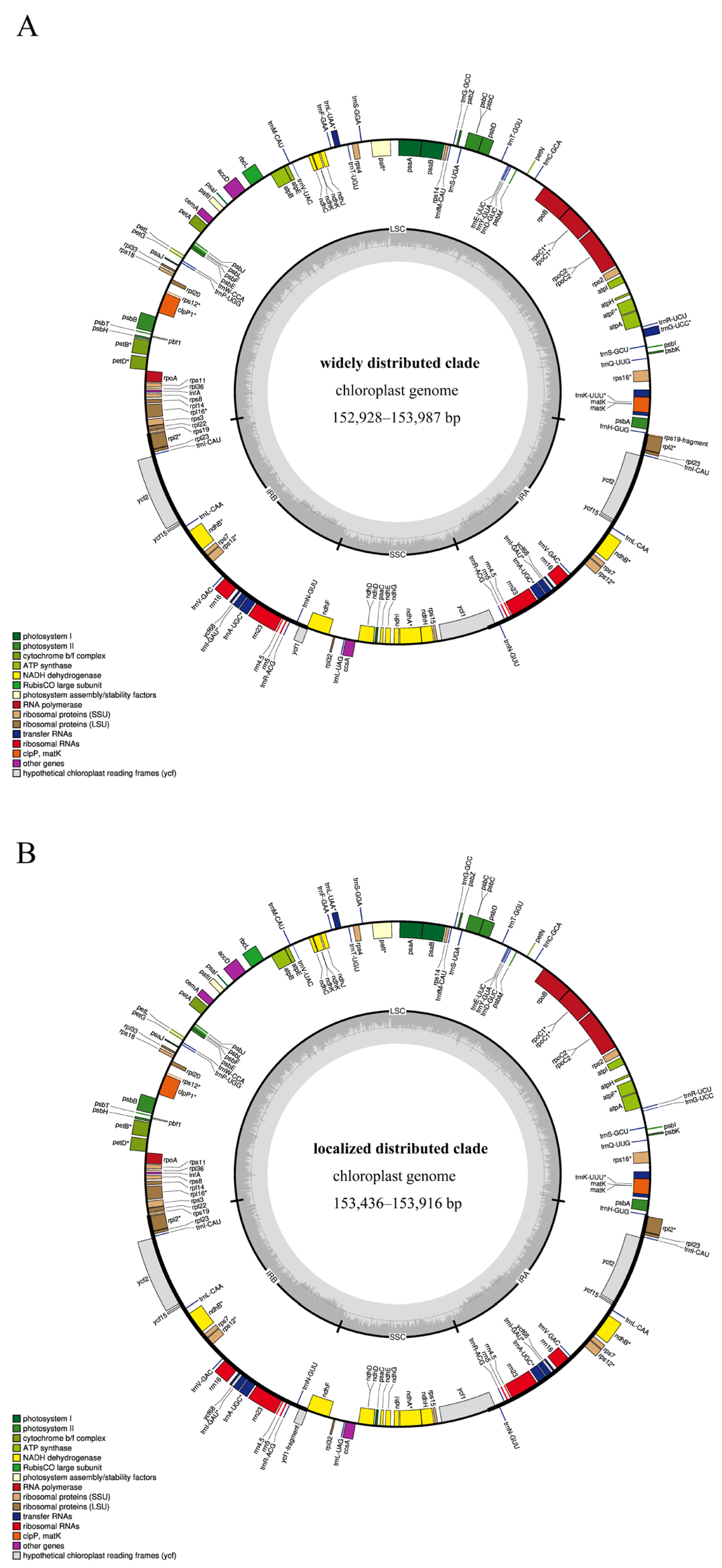
2.1. Features of the Plastome Genome

A total of 24 chloroplast genomes were studied, which belong to two genetically similar evolutionary clades. The large single copy (LSC) region had the greatest variation in length, mainly causing length variation of the chloroplast genome. No large fragment deletions were detected in the inverted repeats (IR) region, and the lengths of two IR regions were consistent in all chloroplast genomes. The GC content of each species was highly similar throughout the entire chloroplast genome, and the same was true for the same regions (LSC, IR, and small single copy, i.e., SSC), though the GC content in IR regions was higher than in other regions.
There were 11 datasets in a widely distributed clade, including L. pauciflorus from Fujian (L. pauciflorus FJ) and Yunnan (L. pauciflorus YN), L. pauciflorus var. ikedae, L. aeschynanthoides, L. pterocaulis, L. heterophyllus from Guizhou (L. heterophyllus GZ) and Guangxi (L. heterophyllus GX), L. wilsonii, L. microphyllus var. omeiensis, L. kwangsiensis and L. heterophyllus var. mollis (Table 1). Chloroplast genome sizes in this clade ranged from 152,928 to 153,987 bp (L. pauciflorus). GC content ranged from 37.43% (L. heterophyllus var. mollis) to 37.49% (L. microphyllus var. omeiensis). LSC length ranged between 84,077 and 85,131 bp, where the smallest was L. pterocaulis and the longest was L. pauciflorus YN. SSC length ranged from 17,746 to 17,922 bp; the smallest was L. kwangsiensis and the longest was L. heterophyllus GX. IR length was in the range of 25,461–25,485 bp. The smallest IR was recorded for L. pauciflorus var. ikedae, while L. pauciflorus YN depicted the longest IR.
There were 13 datasets in the locally distributed clade. Species in this clade included L. gamosepalus, L. pubescens, L. atropurpureus, L. sessilifolius, L. forrestii, L. levipes, L. chatungii, L. guiliangii, L. sp., L. petelotii, L. sulphureoides, L. serratus, and L. metuoensis. Chloroplast genome sizes in this clade ranged from 153,436 to 153,916 bp, with L. atropurpureus having the shortest genome and L. forrestii possessing the longest. GC content ranged from 37.43% to 37.48%, with L. guiliangii possessing the shortest GC content and L. sp. having the longest. LSC length varied from 84,592 to 85,069 bp. L. atropurpureus showed the shortest LSC and the longest was observed in L. forrestii. SSC length ranged from 17,780 to 17,896 bp, the shortest was L. guiliangii, and the longest was L. atropurpureus. IR length was observed within the range of 25,473 to 25,488 bp. L. pubescens had the shortest IR and the longest was observed in L. gamosepalus (Table 2).

2.2. Genome Annotation

All chloroplast genomes owned typical quadripartite structures (Figure 1). A constant number of transfer RNA (36 tRNAs) and ribosomal RNA (4 rRNAs) were observed for all 24 genomes. However, the number of their protein coding sequences (CDs) varied at individual levels, but were similar between the two clades (Table S1).
The widely distributed clade, except for L. heterophyllus GX possessing 79 CDs, exhibited the most prominent variation compared to the others, with the remaining 10 chloroplast genomes all containing 80 CDs. In the locally distributed clade, L. sulphureoides showed 79 CDs, while the remaining 12 chloroplast genomes possessed 80 CDs (Table 2).

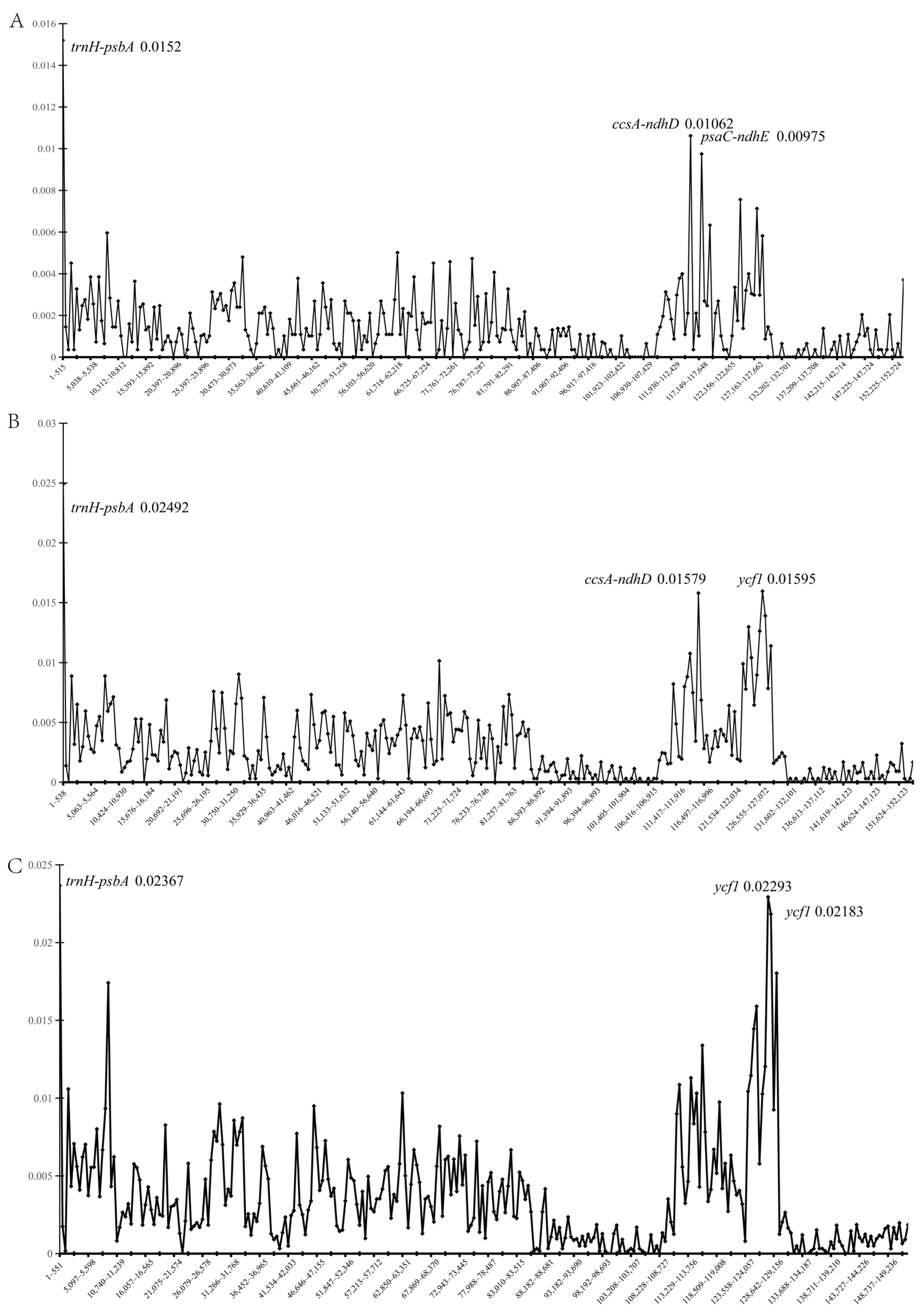
2.3. Genomic Divergence

The IR region displayed a significantly higher degree of sequence conservation in comparison to the single copy region (Figure S1). In contrast, the coding regions exhibited more pronounced evolutionary conservatism compared with the non-coding regions. The distribution of cyan was primarily observed in two reversed repeats within the chloroplast genome. The trends remained consistent across the two regions. The curve exhibited a high peak, and it was positioned closely to the horizontal axis, indicating a diminished level of genetic diversity, consistent similarity, and uniform genetic structure between two reverse repeat regions of 24 chloroplast genomes. The main variation regions included intergenic region spacer (IGS) and CDs, IGS (rps16-trnQ-UUG), IGS (rpoB-trnC-GCA-petN-psbM-trnD-GUC-trnY-GUA-trnE-UUC-trnT-GGU-psbD), IGS (ycf3-trnS-GGA-rps4-trnT-UGU-trnL-UAA-trnF-GAA-ndhJ), IGS (ycf4-cemA), IGS (rpl16), IGS (rps12-rpl32-trnL-UAG-ccsA-ndhD-psaC-ndhE-trnR-UCU-ndhG-ndhI) and CDs (ycf1).
Nucleotide diversity index Pi was used to quantify genetic diversity (Figure 2). The region with the highest average Pi in the widely distributed clade (11 chloroplast genomes) was trnH-psbA (Pi = 0.0152), followed by ccsA-ndhD (Pi = 0.01062) and psaC-ndhE (Pi = 0.00975). In the localized distributed clade (13 chloroplast genomes), trnH-psbA (Pi = 0.02492), ycf1 (Pi = 0.01595) and ccsA-ndhD (Pi = 0.01579) had high Pi. The highly variable regions of both clades contained trnH-psbA and ccsA-ndhD. However, the localized clade exhibited higher genetic diversity and greater sequence differences. The Pi revealed troughs primarily occurring between 82,291–111,930 and 127,662–147,225 in the widely distributed clade, exhibiting low genetic diversity (Figure 2A). The region with low genetic diversity of the localized distributed clade was in the range of 86,393–106,915 and 131,602–147,123 (Figure 2B). The low variation for all 24 chloroplast genomes ranged between 88,681–108,727 and 129,156–149,236 (Figure 2C). These regions were generally inverted repeat regions, consistent with mVISTA results. The Pi of all samples put together was also calculated, with no significant change in the high variable region. In summary, coding regions (except ycf1) were more conservative, with lower Pi values. Non-coding regions usually had higher variation, with higher Pi values.

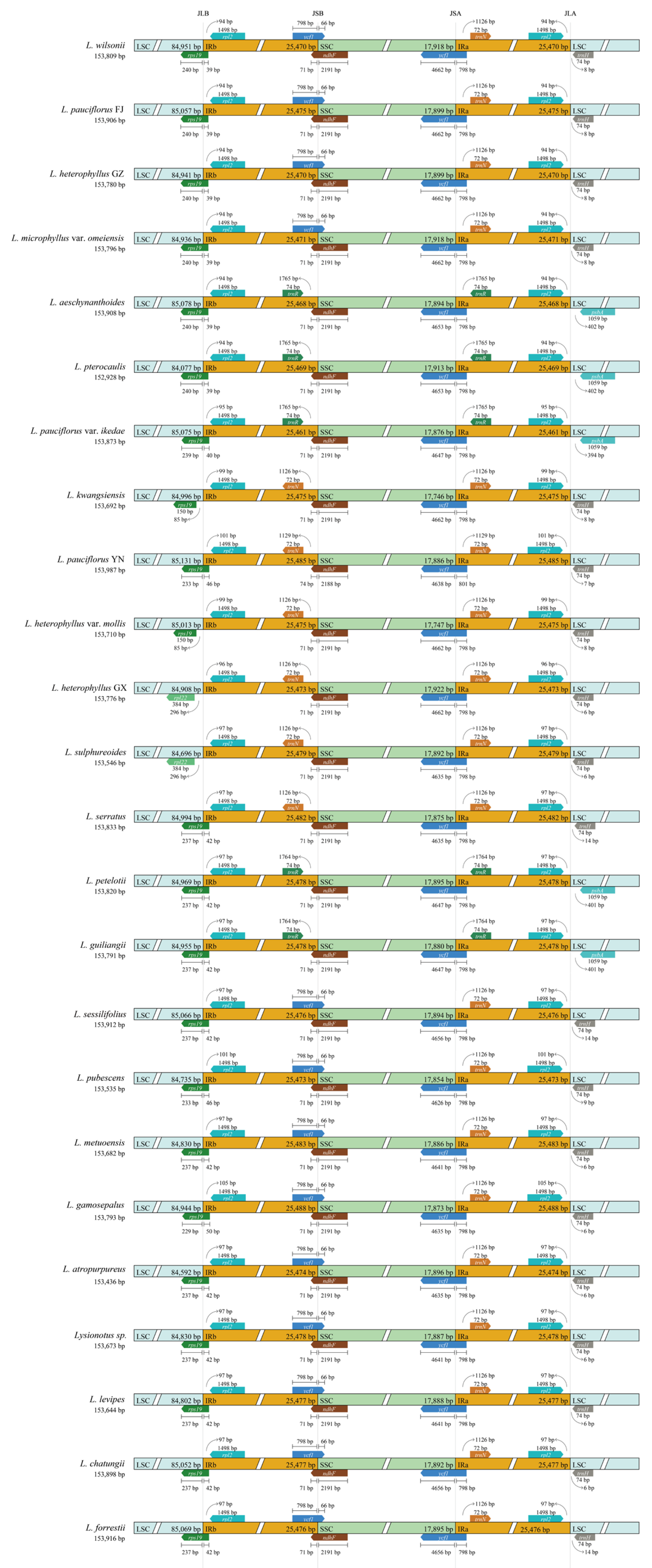
2.4. Contraction and Expansion Analysis of IR Region

The typical quadripartite structure of chloroplast genome results in four boundaries: LSC/IRb (JLB line), IRb/SSC (JSB line), SSC/IRa (JSA line), and IRa/LSC (JLA line). The contraction/expansion of IR region caused evolution and variations in chloroplast GC content and genome size of plant. IR region variation was related to species’ relationship, geographical distribution and ecological adaptation. To better understand the impact of gene transfer or indel events, both within and outside the IR region, we examined the chloroplast genome features of 24 samples and evaluated the phenomenon of IR contraction and expansion.
According to CPJSdraw, arrows depict the distance between the start and end of a gene from the junction site. The scale bar on the upper or lower parts of the genes extending from one region to another illustrates the number of base pairs to which genes are connected in that specific region. The rps19, ndhF, ycf1, and trnH genes were located at LSC/IRb, IRb/SSC, SSC/IRa, and IRa/LSC regions, respectively (Figure 3) in most of the chloroplast genomes. The rps19 gene was detected in 22 chloroplast genomes, and L. kwangsiensis and L. heterophyllus var. mollis were completely located in the LSC region. L. heterophyllus GX in the widely distributed clade, and L. sulphureoides in the locally distributed clade, missed the rps19 gene, which was replaced by the rpl22 gene located in the LSC region with 296 bp apart from JLB line.
Excluding L. heterophyllus GX, L. kwangsiensis and L. heterophyllus var. mollis in the widely distributed clade, the rps19 gene in another 8 chloroplast genomes spanned between the LSC and IRb regions, and the distances between rps19 and JLB line ranged from 233 to 240 bp. The ndhF gene was located in the SSC region, with a distance of 2188–2191 bp from the JSB line (boundary between IRb and SSC). In addition, L. wilsonii, L. pauciflorus FJ, L. heterophyllus GZ, and L. microphyllus var. omeiensis had ycf1 pseudogenes in IRb and also contained 72 bp trnN gene in IRa region. L. aeschynanthoides, L. aeschynanthoides and L. pauciflorus var. ikedae each conained 74 bp trnR gene in IRb and IRa regions. L. kwangsiensis, L. pauciflorus YN, L. heterophyllus var. mollis and L. heterophyllus GX each exhibited 72 bp trnN gene in IRb and IRa regions.
Except for L. sulphureoides in the locally distributed clade, the rps19 gene in 12 chloroplast genomes was located on LSC and IRb regions, and the distances between rps19 and JLB line ranged from 229–237 bp. The distance of ndhF in the SSC region to JSB line was 2191 bp for 13 chloroplast genomes, which were more conserved compared with the widely distributed clade. Most of the species in the localized clade, such as L. sessilifolius, L. pubescens, L. metuoensis, L. gamosepalus, L. atropurpureus, L. sp., L. levipes, L. chatungii and L. forrestii, had ycf1 pseudogene in IRb region and 72 bp trnN gene in IRa region at the same time. L. petelotii and L guiliangii had 74 bp trnR gene in IRb and IRa regions. L. sulphureoides and L. serratus had 72 bp trnN gene in IRb and IRa regions. The length of trnR and trnN genes was highly conserved both the clades.
TrnH served as the boundary between the IRa and SSC regions, which was consistent with previous studies. L. aeschynanthoides, L. pterocaulis and L. pauciflorus var. ikedae in the widely distributed clade lost trnH gene (these three species had 74 bpd trnR gene in IRb and IRa regions, respectively). Similarly, trnH genes were also lost in L. petelotii and L. guiliangii in the locally distributed clade, while trnH in other samples were located in LSC region with 74 bp distance away from the JLA line. In summary, chloroplast genome evolution in the widely distributed clade and the locally distributed clade was relatively conservative. The ndhF was a relatively stable boundary gene with a broader distance range from JSB line in the widely distributed clade (2188–2191 bp). Samples in the localized distributed clade had a similar structure because the ndhF had the same distance from JSB (2191 bp). The variation range of boundary gene length in the widely distributed clade and the diversity of genes on two sides of the boundary provided more possibilities for IR boundary expansion/contraction.

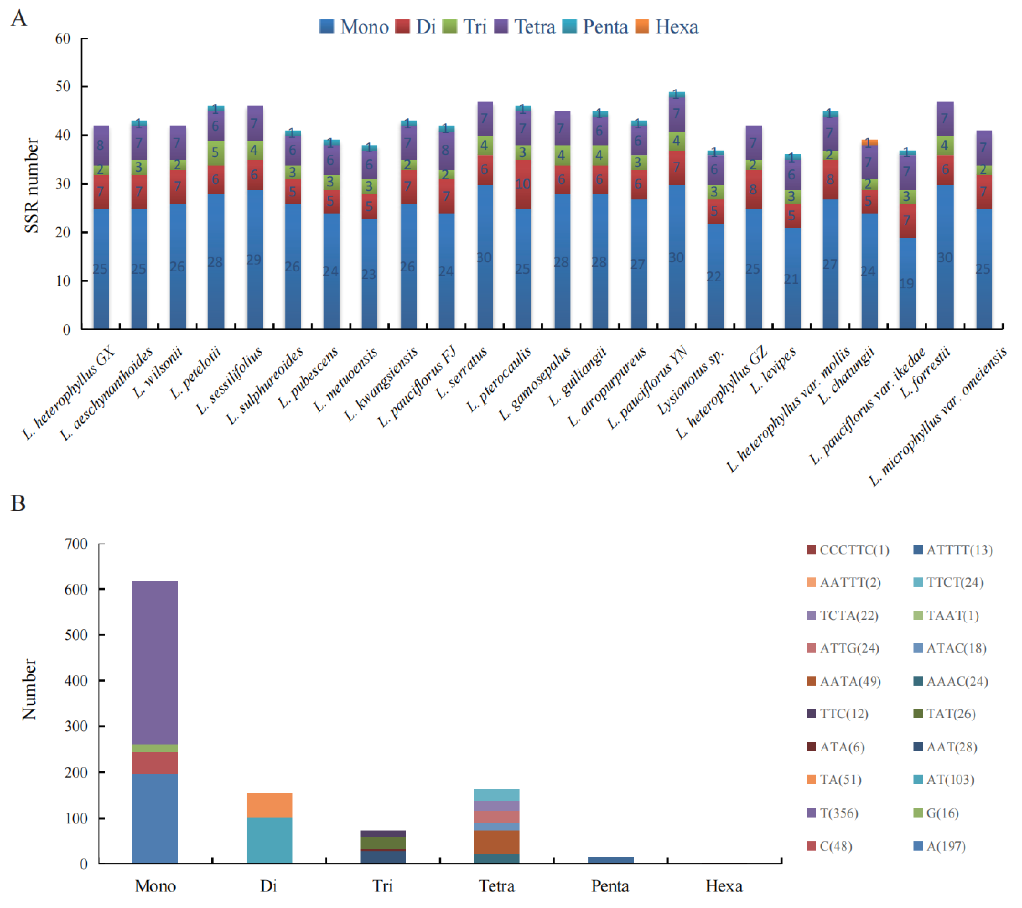
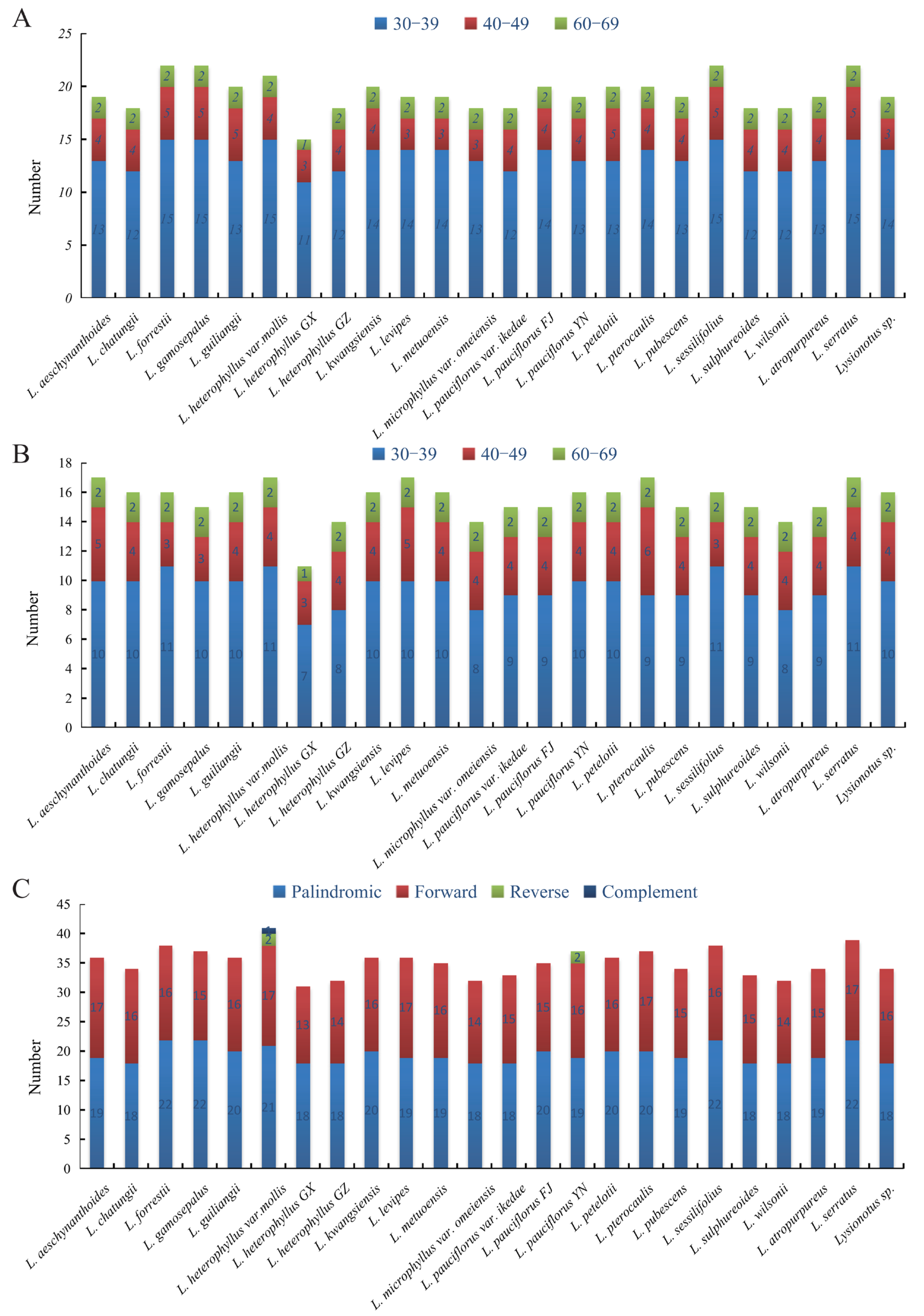
2.5. Repeat Analysis

We compared the SSRs of 24 chloroplast genomes to understand overall distribution, types, and the number of highly similar repeats in widely and locally distributed clades (Table S2). The number of SSRs identified in the 24 chloroplast genomes ranged from 36 to 49 (Figure 4A). Mononucleotides, dinucleotides, trinucleotides and tetranucleotides were prevalent in 24 chloroplast genomes. A total of four types of mononucleotides were detected, with a large difference in number. The most abundant mononucleotides were T (356 polythymine), followed by A (197 polyadenine), C (48 polycytosine), and G (16 polyguanine). A total of two types of dinucleotides were detected, including 103 ATs and 51 TAs. A total of four types of trinucleotides were detected, including AAT, ATA, TAT and TTC, with 28, 6, 26 and 12 repeat numbers, respectively. Seven types of tetranucleotides included AATA, AAAC, ATAC, ATTG, TAAT, TCTA and TTCT, with repeat numbers of 49, 24, 18, 24, 1, 22 and 24, respectively. Pentanucleotides were present in L. aeschynanthoides, L. petelotii, L. sulphureoides, L. pubescens, L. metuoensis, L. kwangsiensis, L. pauciflorus FJ, L. pterocaulis, L. guiliangii, L. atropurpureus, L. pauciflorus YN, L. sp. MT, L. levipes, L. heterophyllus var. Mollis and L. pauciflorus var. ikedae. ATTTT and AATTT were two different types of pentanucleotides, with repeat numbers of 13 and 2, respectively. Only one hexanucleotide repeat CCCTTC was detected, and it existed in L. chatungii (Figure 4B).
We detected 32–41 pairs of LRSs, greater than 30 bp, consisting of forward repeats (F), reverse repeats (R), complementary repeats (C), and palindromic repeats (P) in 24 Lysionotus chloroplast genomes (Table S3). The LRSs number of the widely distributed clade ranged from 32 to 41 bp, whereas the number of the localized distributed clade ranged from 33 to 39 bp. Among these LRSs, the number of forward and palindrome repeats were considerably higher than reverse and complement repeats. Except for L. heterophyllus var. mollis (four LRSs, P, F, R, and C) and L. pauciflorus YN (three LRSs, P, F, and R), the other 22 chloroplast genomes only contained two LRSs, i.e., P and F. The number of forward repeat lengths per interval (30–39 bp, 40–49 bp and 60–69 bp) were shown in Figure 5A.
The number of palindromic repeats in 24 chloroplast genomes was higher than forward repeats, and the length was mainly 30–39 bp. Figure 5B shows the number of palindromic repeats in each chloroplast genome, with sizes being set in three intervals: 30–39 bp, 40–49 bp and 60–69 bp. The palindromic repeats number of 24 chloroplast genomes among 30–39 bp ranged from 11–15 bp. The number of palindromic repeats for the widely distributed clade ranged from 11 to 15 bp, while it was 12–15 bp for the localized distributed clade. The number of forward repeats of each chloroplast genome in 30–39 bp interval was at least 7 F and 11 F at most (Figure 5C). The number in the widely distributed clade was in the range of 7–11 bp, and the number in locally distributed clade ranged from 9 to 11. In summary, the widely distributed clade dominated a broader range of palindromic repeat numbers (11–15) and forward repeat numbers (7–11) in the 30–39 bp interval (versus the localized distributed clade: 12–15 P, 9–11 F). Furthermore, L. pauciflorus YN and L. heterophyllus var. mollis also belonged to the widely distributed clade and possessed more abundant types of LRSs, suggesting that the widely distributed clade may possess more special structures or functions, such as potential adaptability.

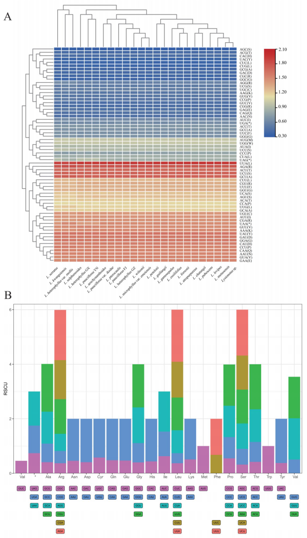
2.6. Codon Usage Bias Pattern

The number of codons encoding the same amino acid was more conserved across Lysionotus species. L. atropurpureus in the locally distributed clade exhibited a higher frequency compared to codons in other species. However, the number of codons encoding different amino acids varied greatly. Among 64 codons in 24 chloroplast genomes, there were 30 more preferred codons (relative synonymous codon usage, ie., RSCU > 1), two equally preferred codons (RSCU = 1) (UGG and AUG), and 32 less preferred codons (RSCU < 1) (Figure 6A). In the widely distributed clade, AUA encoding isoleucine (Ile) was the most abundant (1095 in L. kwangsiensis), while the UGU encoding cysteine (Cys) was the least (80 in both L. aeschynanthoides and L. pterocaulis). Additionally, there were 135,446 codons ended with A/U and 140,586 codons ended with G/C. In the locally distributed clade, UAU encoding tyrosine (Tyr) was the most abundant (2092 in L. atropurpureus), and GCA encoding alanine (Ala) showed the least abundance (78 in L. petelotii, L. sulphureoides and L. guiliangii). Additionally, there were 172,087 codons ended with A/U and 178,439 codons ended with G/C (Table S4). Based on RSCU and observed frequency, the codon usage was biased for G/C endings in two different clades.
The RSCU of 64 codons (including UAA, UAG and UGA stop codons) encoding amino acids are shown in Figure 6B, where each column represents an amino acid. Leucine (Leu), arginine (Arg) and serine (Ser) featured the highest total RSCU (RSCU = 6), these amino acids were biased to use UUG, UUA and CUU for leucine (Leu); CGU, CGA and AGA for arginine (Arg); and UCU, UCA and AGU for serine (Ser). Followed by alanine (Ala), glycine (Gly), proline (Pro), threonine (Thr) and valine (Val), these amino acids featured a total RSCU of 4. Alanine (Ala) was biased to use GCU and GCA, glycine (Gly) was biased to use GGU and GGA, and proline (Pro) was biased to use CCU and CCA. Threonine (Thr) was biased to use ACU and ACA, and valine (Val) was biased to use GUU and GUA. Moreover, asparagine (Asn) exhibited a preference for the AAU codon, the GAU codon was inclined towards aspartate (Asp), cysteine (Cys) was biased to use UGU, glutamine (Gln) showed tendency towards CAA, glutamic acid (Glu) was biased to use GAA, histidine (His) was inclined towards CAU, lysine (Lys) preferred to use AAA, UUU was employed by phenylalanine (Phe) and tyrosine (Tyr) was biased to use UAU. Isoleucine (Ile) was encoded by three different codons, but only AUU was greater than 1 (RSCU = 1.47). Methionine (Met) and tryptophan (Trp) were encoded by AUG and UGG, and these two codons were equally preferred codons (RSCU = 1).

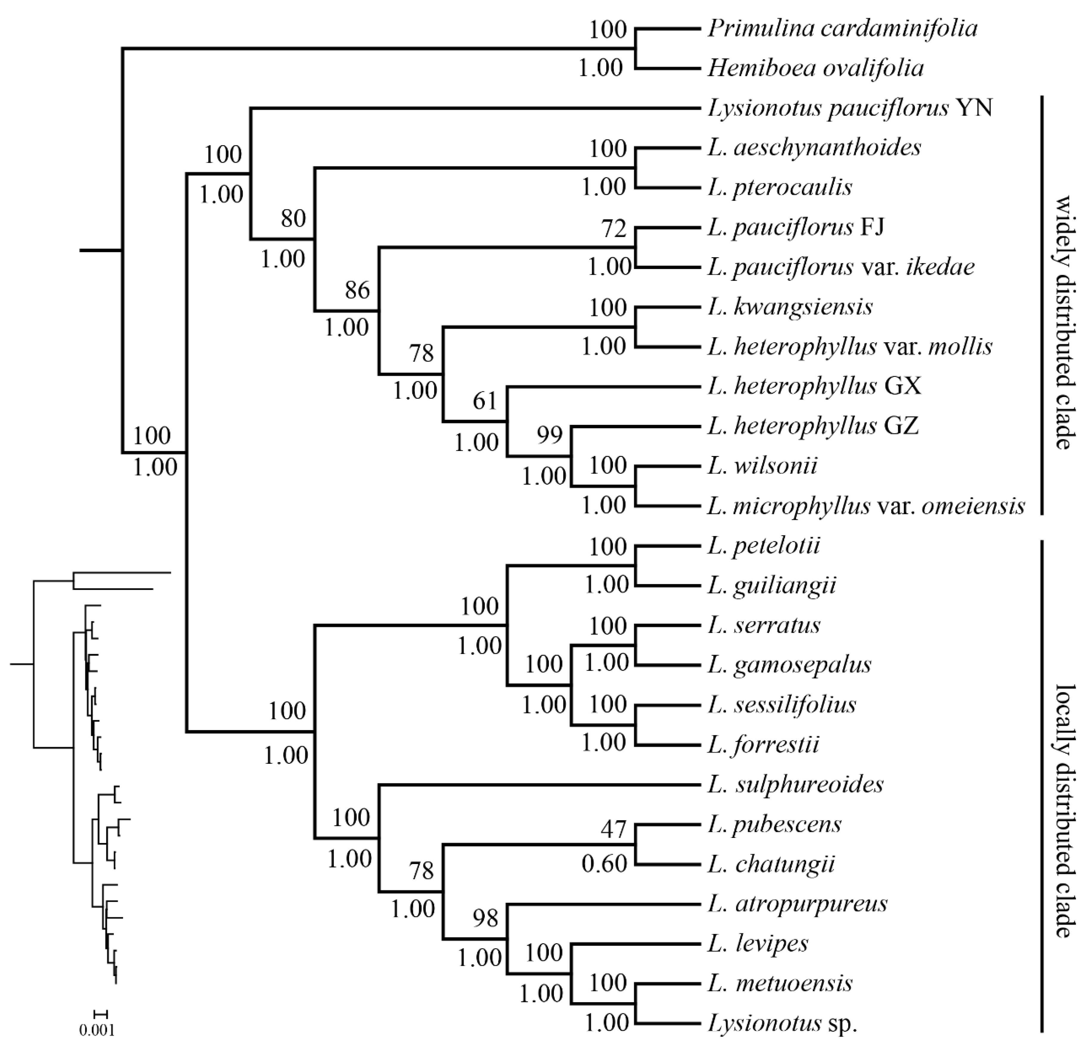
2.7. Phylogenetic Relationships

Choosing Hemiboea ovalifolia and Primulina cardaminifolia as outgroups, 24 samples in this study formed two clades; the phylogenetic relationship is shown in Figure 7. The support rates of ML and posterior probabilities of BI trees were marked above and below the branches in joint support tree. The morphological characteristics of some representative species are shown in Figure 8, where panels A–F depict species in the widely distributed clade (e.g., L. pauciflorus and L. heterophyllus), and panels G–P illustrate species in the locally distributed clade (e.g., L. atropurpureus and L. sessilifolius). In the first widely distributed clade, L. pauciflorus from Yunnan separated earliest, followed by L. aeschynanthoides and L. pterocaulis, which further clustered together. The L. pauciflorus from Fujian and L. pauciflorus var. ikedae further clustered together. L. kwangsiensis and L. heterophyllus var. mollis, both from Guangxi, diverged at a relatively intermediate stage and exhibited a closer phylogenetic relationship within their clade. In contrast, L. heterophyllus from Guizhou and Guangxi, L. wilsonii from Sichuan, and L. microphyllus var. omeiensis from Chongqing, diverged most recently, as shown by their terminal positions in the phylogenetic tree.
Species in the second locally distributed clade could further form two groups, the first group including six species: L. petelotii, L. guiliangii, L. serratus, L. gamosepalus from, L. sessilifolius and L. forrestii. The second group includes seven species: L. sulphureoides and L. pubescens, L. sulphureoides, L. atropurpureus, L. levipes and L. sp. Despite the geographical proximity of Sichuan and Tibet, the phylogenetic relationship of species from the two regions was relatively distant, and they evolved relatively independently in different clades. Moreover, although species L. gamosepalus, L. atropurpureus, L. metuoensis and Lysionotus sp. were both from Motuo, L. gamosepalus was more closely related to L. serratus from Guangxi, while L. atropurpureus possibly experienced a more complex evolution, and underwent adaptive evolution in the Tibet.
The species in the second local clade can be divided into two groups. The first group consists of six species: L. petelotii, L. guiliangii, L. serratus, L. gamosepalus, L. sessilifolius, and L. forrestii. The second group includes seven species: L. sulphureoides, L. pubescens, L. atropurpureus, L. levipes, and an unidentified species of L. sp. Despite the geographical proximity of Sichuan and Tibet, the phylogenetic relationships among species from these two regions are relatively distant, indicating that they have evolved independently in different clades. Furthermore, although L. gamosepalus, L. atropurpureus, L. metuoensis, and L. sp. all originate from Motuo, L. gamosepalus is more closely related to L. serratus from Guangxi. In contrast, L. atropurpureus appears to have undergone a more complex evolutionary process, possibly undergoing adaptive evolution in Tibet. This analysis suggests that, despite their proximity, the species from different regions may exhibit significant phylogenetic divergence due to differences in their environments, ecologies, and evolutionary histories.

2.8. Positive Selection Based on Chloroplast

Among the 78 single-copy CDS genes initially considered for positive selection analysis (Table S1), 69 genes were ultimately selected (Table 3). Among all the genes, only the rbcL gene was detected to be under significant positive selection (p = 8.77 × 10⁻⁴). No significant positive selection was detected in other genes (p-value > 0.05). This may indicate that the rbcL gene has experienced special selective pressure during the evolutionary process of the species. This may be because the biological functions in which it is involved, such as those related to photosynthesis, play an important role in the species’ adaptability to the current environment. As a result, it has been favored by natural selection, and its gene frequency may have changed significantly in the population to adapt to the environment.
However, in the Bayesian Empirical Bayes (BEB) test, codon sites in 10 genes were found to have high posterior probabilities (atpA, cemA, clpP, ndhA, ndhB, ndhC, ndhE, ndhH, rps8, and ycf1) (Table 3). Previous studies have shown that codon sites with high posterior probabilities should be considered as positively selected sites [39], implying that these 10 genes might also be under positive selection pressure [38]. They have undergone adaptive changes during the differentiation of the widely distributed clade and the locally distributed clade in Lysionotus, although such changes did not reach statistical significance in traditional positive selection tests based on p-values.

3. Discussion

3.1. Chloroplast Genome Structure and Evolutionary Conservation

This study presents the first comprehensive comparative analysis of chloroplast genomes across 24 Lysionotus species, revealing that all genomes possess the canonical quadripartite structure, consistent with the single-species analysis of L. pauciflorus reported by Ren et al. [40]. Notably, the variation in genome length between the widely distributed and locally distributed clades is primarily attributed to differences in the large single-copy (LSC) region, rather than expansions or contractions of the inverted repeat (IR) regions. This pattern contrasts with that observed in many angiosperms, where IR variation typically drives genome size changes [29]. The remarkable conservation of IR regions is likely linked to their inclusion of rRNA gene clusters, which are essential for ribosomal function, as further supported by their elevated GC content (43.14–43.19%). Furthermore, the absence of gene rearrangements or large fragment deletions underscores the exceptional structural stability of Lysionotus chloroplast genomes, contrasting sharply with the more dynamic plastomes observed in other Gesneriaceae genera such as Henckelia [32,41].

3.2. Hypervariable Regions and Ecological Adaptation

Through mVISTA alignment and nucleotide diversity analyses, we identified trnH-psbA and ccsA-ndhD as shared hypervariable regions across both clades, while the ycf1 gene exhibited notably higher divergence within the locally distributed species. These findings reinforce the utility of ycf1 as an effective species-discriminating marker, as previously suggested by Shaw et al. [28]. The elevated genetic diversity observed in locally distributed clades, exemplified by L. atropurpureus, likely reflects adaptation to the heterogeneous microhabitats of the Himalayan region. In contrast, the relatively low variation in widely distributed species such as L. pauciflorus suggests a more generalized environmental adaptation. Interestingly, non-coding regions exhibited greater variability than coding regions, consistent with relaxed selective constraints on intergenic spacers. The trnH-psbA region, involved in photosystem II assembly, may underpin adaptive differentiation in light-harvesting efficiency, whereas the potential role of ccsA-ndhD (implicated in cytochrome c biosynthesis) variations in high-altitude adaptation warrants further functional validation [19].

3.3. Phylogenetic Insights: Comparison with Previous Studies

Previous phylogenetic trees of Lysionotus based on nuclear ITS and chloroplast trnL-F sequences resolved two major clades but showed limited resolution within clades [37]. In contrast, our chloroplast genome-based phylogenetic analysis (Figure 7) provides higher resolution, and exhibits overall topological congruence with the phylogeny constructed using 649 orthologous genes [42]. Only a few species show discordant phylogenetic relationships. For example, L. atropurpureus clusters with L. levipes in the chloroplast tree, whereas it diverges earliest as a basal lineage in the nuclear gene tree, being closely related to L. serratus and L. gamosepalus. This discrepancy may be attributed to incomplete lineage sorting or historical hybridization events.
In this study, the early divergence of L. pauciflorus from Yunnan and the close clustering of Fujian populations with L. pauciflorus var. ikedae likely resulted from geographic isolation driven by enhanced East Asian monsoons during the Miocene. The Yunnan population evolved independently due to the topographic barrier of the Hengduan Mountains, while Fujian populations dispersed to Japan via land bridges during the Pleistocene, forming the variety. Notably, L. gamosepalus from Medog, Tibet, clusters with L. serratus from Guangxi rather than sympatric L. atropurpureus, implying long-distance dispersal during the Himalayan orogeny or ecological niche conservatism in karst habitats. This pattern challenges the hypothesis of strict geographic structuring proposed by Monro et al. [33]. Thus, chloroplast genome phylogeny reveals complex evolutionary histories masked by previous analyses using limited molecular markers.

3.4. Research Limitations and Future Directions

This study has several limitations. First, sampling covers approximately 70% of Lysionotus species, lacking representation of Southeast Asian endemics (e.g., Vietnamese taxa), which may constrain genus-wide evolutionary inferences. Second, the functional associations between identified hypervariable regions and adaptive traits such as epiphytism remain unexplored. Third, potential conflicts between nuclear and plastid phylogenies, influenced by processes like polyploidy and hybridization, were not addressed, although these phenomena could bias chloroplast-based phylogenies. Future research should aim to (1) sequence the remaining species to complete genus-wide plastome diversity, (2) integrate transcriptomic data to elucidate functional links between hypervariable regions and environmental adaptation, and (3) incorporate nuclear genomic data to resolve reticulate evolution, particularly in locally distributed clades with complex biogeographic histories.

3.5. Novel Contributions and Conservation Implications

This work represents a pioneering large-scale comparative plastome analysis within Lysionotus, revealing distinct patterns of genomic stability and variation between the two major clades. The identification of hypervariable regions such as trnH-psbA provides valuable molecular markers for species identification and germplasm screening. Moreover, our phylogenetic findings offer a molecular framework to guide conservation prioritization, exemplified by the recognition of independent evolutionary lineages in the Himalayan biodiversity hotspot (e.g., L. atropurpureus and L. metuoensis). By linking genomic variation to ecological distribution patterns, this study provides methodological insights for adaptive evolution research in Gesneriaceae and lays a theoretical foundation for the sustainable utilization of this ornamental and medicinally important genus.

4. Materials and Methods

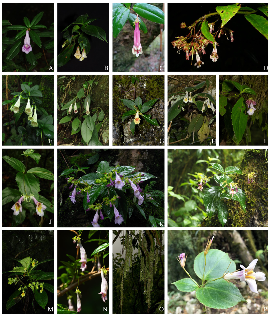
4.1. Plant Materials

In this study, a total of 11 samples from a widely distributed clade and 13 samples from a locally distributed clade were compared, representing a total of 24 chloroplast genomes from the Lysionotus species. The sampling strategy was mainly based on the phylogenetic relationship obtained by Huang [43] based on nuclear ITS and chloroplast trnl-F, further combined with the actual situation of scientific investigation. The widely distributed clade contained L. heterophyllus GX, L. aeschynanthoides, L. wilsonii, L. kwangsiensis, L. pauciflorus FJ, L. pterocaulis, L. pauciflorus YN, L. heterophyllus GZ, L. heterophyllus var. mollis, L. pauciflorus var. ikedae, L. microphyllus var. omeiensis, both samples for L. heterophyllus and L. pauciflorus. The locally distributed clade contained L. pubescens, L. atropurpureus, L. sessilifolius, L. forrestii, L. levipes, L. chatungii, L. guiliangii, L. petelotii, L. sulphureoides, L. serratus, L. metuoensis, L. gamosepalus, also including one Lysionotus sp. from Motuo China. Table 1 indicates detailed information for newly sequenced plants. Voucher specimens of each collected species were deposited at Herbarium of Guangxi Institute of Botany (IBK) Guangxi Institute of Chinese Academy of Science. They were identified by Professor Weibin Xu.

4.2. DNA Extraction and Sequencing

Fresh samples were collected from natural habitat sites and planted in the germplasm garden of Guangxi Institute of Botany. Our collection of plant materials complied with institutional, national and international guidelines. The tissues were immediately preserved in discolored silicone and total DNA was extracted with the NuClean Plant Genomic DNA Kit from CWBIO. The quantity was evaluated by 1.0% (w/v) agarose gel electrophoresis SYBR Green I and Nanodrop2000 (Thermo Fisher Scientific, Waltham, MA, USA) to assess the concentration and purity of the DNA samples. Then, the DNA library was constructed at 250 to 300 bp, with DNA fragments converted into Illumina high-throughput sequencer-compatible forms. The high-throughput sequencing was performed on the Illumina Nova6000 Platform (Illumina, San Diego, CA, USA) and produced a total of 6 Gb of raw data each sample.

4.3. Plastome Genome Assembly and Annotation

The raw data were assembled under Linux using GetOrganellev1.7.5 [44], the parameters were set to get_organelle_from_reads. py-1 G_R1_001.fastq.gz-2 G_R2_001.fastq.gz -o G_output -R 45 -k 21,33,45,55,65,73,85,105,125 -f embplant_pt -t 10. The starting point of the chloroplast genomes was adjusted using seqkit [45] (version 0.12.1), and the depth of coverage was detected using bwa [46] (version 0.7.17) and samtools [47] (version 1.17) software. Sequence mapping analysis and Bandage_Windows [48] (version 0.8.1) was employed to judge the assembly quality. All 24 chloroplast genomes were assembled to obtain complete chloroplast rings. Then, the appropriate assembly fasta files were selected using Gepard [49] (version 1.40). The CPGAVAS2 [50] (version 2.1.0) and Geseq [51] (version 2.0.0) were combined to annotate the chloroplast genome, and the annotated results were manually adjusted to refer to NC_082151.1. Finally, the chloroplast genome was mapped by OGDRAW [52] (version 1.3.1).

4.4. Genome Comparison

Use CPJSdraw [53] (version 1.0.0) to visualize the junction boundary of quadripartite regions of the chloroplast genome, and compare the structure of the chloroplast genome.
To compare genome structures and sequence similarities among the 24 complete Gesneriaceae plastomes, sequences were aligned by Shuffle-LAGAN64 [54,55,56,57] (version 2.0.0), which could detect rearrangement, and analyze using mVISTA “http://genome.lbl.gov/vista/mvista/submit.shtml (accessed on 20 September 2023)”.
To quantify genetic diversity concretely, sequence polymorphism analysis of the 24 chloroplast genomes was performed on Dna SP [58] (version 6.15.03). A sliding window was performed every 500 bp, and one Pi was calculated every 500 bp. That is, 500 bp window length and 500 bp step size were set as the sliding window.

4.5. Repeats Analysis

MISA “https://webblast.ipk-gatersleben.de/misa/ (accessed on 20 September 2023)” was used to detect the chloroplast SSRs in 24 Lysionotus chloroplast genome sequences. The minimum numbers of repeats for mononucleotide, dinucleotides, trinucleotides, tetranucleotides, pentanucleotide, and hexanucleotides were 10, 5, 4, 3, 3, and 3, respectively [59,60,61].
REPuter “https://bibiserv.cebitec.uni-bielefeld.de/reputer/ (accessed on 20 September 2023)” was performed to identify large repeat sequences, reaching the following four repeat categories: forward, reverse, complement and palindromic repeats. The parameters were as follows: (1) setting Hamming distance as 3, (2) maximum computed repeats as 5000, and (3) minimal repeat size as 30.

4.6. Phylogenetic Analysis

In order to deeply understand the evolutionary relationship between the widely distributed clade and the locally distributed clade, 72 common single-copy CDs in 24 complete chloroplast genomes were extracted in PhyloSuite [62] (version 1.2.2) and performed for phylogenetic analysis. Each extracted gene was aligned with MAFFT [63] (version 7.526) and ModelFinder [64] (version 1.6.8) software was used to identify the best-fit nucleotide substitution model for the matrix based on Akaike information criterion (AIC). Maximum likelihood phylogenetices were inferred using IQ-TREE [65] (version 2.3.0) under GTR+F+I model for 1000 ultrafast bootstraps. Bayesian inference phylogenetices were inferred using MrBayes [66] (version 3.2.6), assuming different probabilities of substitution between each pair of nucleotides and accounting for rate heterogeneity among sites, i.e., the substitution rates of all sites were not equal or did not follow the same distribution. Setting Statefreqpr to Fixed (Empirical), and the Markov Chain Monte Carlo (MCMC) algorithm was employed to generate posterior probability distribution and the phylogenetic tree. The iterations number of the MCMC chain algorithm was 200,000, the output information was printed every 1000 iterations, and one sample was extracted from the MCMC chain every 1002 iterations. Two parallel sets were run in MCMC chains for Bayesian analysis, with checkpoints being saved every 5000 iterations. There were four MCMC chains in each run: one was a hot chain and the other three were cold chains, each chain starting from a different initial point, and samples were exchanged to avoid falling into local optimality, improving MCMC sampling efficiency and convergence. We summarized the MCMC sampling results using relative burn-in, discarding 27% samples, and resampling trees and parameters after the log probability stabilized, to avoid influence of the initial state on the posterior probability distribution. We evaluated all parameters in the model based on convergence diagnostics provided by the ‘sump’ and ‘sumt’ commands. Finally, we assessed the consistency and stability between different runs using the estimated effective sample size (ESS) and the potential scale reduction factor (PSRF).

4.7. Positive Selected Analysis

For the 24 species, single-copy CDS sequences were aligned by projecting onto corresponding amino acid alignments generated using MUSCLE [67] (version 3.8.425). The alignments were systematically evaluated for gap frequencies to assess data quality. Corresponding DNA codon alignments were subsequently refined using TRIMAL [68] (version 1.4.0) to generate high-quality, reliable alignments suitable for downstream positive selection analyses. To detect positive selection acting on individual codons along the specified lineages of U. rockii and U. henryi, the optimized branch-site model in the CODEML program of PAML [69] (version 4.10.7) was employed. Selective pressure was quantified by the nonsynonymous (dN)/synonymous (dS) substitution rate ratio (ω), where ω > 1 indicates positive selection, ω = 1 denotes neutral evolution, and ω < 1 suggests purifying selection [70]. Log-likelihood values were calculated under an alternative branch-site model (Model = 2; NSsites = 2; Fix = 0), allowing ω to vary among codons along target branches, and a null model (Model = 2; NSsites = 2; Fix = 1; Fixω = 1), enforcing neutral evolution (ω = 1) at all sites. Likelihood ratio tests (LRTs) were performed by comparing these models, with statistical significance assessed via a one-degree-of-freedom right-tailed chi-square test. p-values were adjusted for multiple comparisons [71]. Genes with adjusted p-values < 0.05 and identified positively selected sites were designated as positively selected genes (PSGs). The Bayesian Empirical Bayes (BEB) approach was applied to estimate posterior probabilities of site classes for pinpointing specific codon sites under positive selection. Codon sites with high posterior probabilities were identified as positively selected sites [38].

5. Conclusions

This is the first report comparing the complete chloroplast genome between 11 widely distributed and 13 locally distributed Lysionotus species. In this study, all 24 chloroplast genomes had typical quadripartite structure, and the number of CDs, rRNA and tRNA varied at the individual level, but were similar between the two clades. Species in the widely distributed clade had a broader length variation range in genome, LSC, SSC and IR boundary gene, while it was poorer in repeat sequence type and genetic diversity, indicating they had simple genetic variation were even more vulnerable to adverse factors. Species in the locally distributed clade owned richer repeat sequence types and higher genetic diversity. Phylogenetic analysis showed species in the locally distributed clade could form two further groups.

Supplementary Materials

The following supporting information can be downloaded at https://www.mdpi.com/article/10.3390/ijms26157031/s1.

Author Contributions

Conceptualization, investigation, resources, and data curation, W.-B.X.; software, formal analyses, visualization, writing—original draft preparation, J.-H.L.; writing—review and editing, C.-H.G., J.-H.L. and W.-B.X.; supervision, C.-H.G.; funding acquisition, W.-B.X. All authors have read and agreed to the published version of the manuscript.

Funding

This work was supported by the National Natural Science Foundation of China (No. 31860043).

Institutional Review Board Statement

Not applicable.

Informed Consent Statement

Not applicable.

Data Availability Statement

The data generated in this study are available at Genbank (accession numbers: PQ468967-PQ468996 and PQ433130).

Acknowledgments

We sincerely thank Jie Huang for her valuable assistance in improving our paper. We also express our gratitude to Meng-Qi Han, Xin-Xin Zhu, Lei Cai, Fang Wen, and Wen-Guang Wang for kindly providing some photos of Lysionotus.

Conflicts of Interest

The authors declare no conflicts of interest.

References

  1. Harlan, J.R. Agricultural Origins: Centers and Noncenters. Science 1971, 174, 468–474. [Google Scholar] [CrossRef] [PubMed]
  2. Tanksley, S.D.; McCouch, S.R. Seed Banks and Molecular Maps: Unlocking Genetic Potential from the Wild. Science 1997, 277, 1063–1066. [Google Scholar] [CrossRef] [PubMed]
  3. Zeder, M.A.; Emshwiller, E.; Smith, B.D.; Bradley, D.G. Documenting domestication: The intersection of genetics and archaeology. Trends Genet. 2006, 22, 139–155. [Google Scholar] [CrossRef] [PubMed]
  4. Meyer, R.S.; Purugganan, M.D. Evolution of crop species: Genetics of domestication and diversification. Nat. Rev. Genet. 2013, 14, 840–852. [Google Scholar] [CrossRef]
  5. Ford-Lloyd, B.V.; Schmidt, M.; Armstrong, S.J.; Barazani, O.Z.; Engels, J.; Hadas, R.; Hammer, K.; Kell, S.P.; Kang, D.; Khoshbakht, K.; et al. Crop Wild Relatives—Undervalued, Underutilized and under Threat? BioScience 2011, 61, 559–565. [Google Scholar] [CrossRef]
  6. Ma, J.; Li, Z.-Y.; Wang, Y.-Z.; Wang, W.-T.; Pan, K.-Y. Plants of Gesneriaceae in China. Taxon 2005, 54, 574. (In Chinese) [Google Scholar] [CrossRef]
  7. Wang, K.; Zhang, C.; Chen, H.; Yue, Y.; Zhang, W.; Zhang, M.; Qi, X.; Fu, Z. Karst landscapes of China: Patterns, ecosystem processes and services. Landsc. Ecol. 2019, 34, 2743–2763. [Google Scholar] [CrossRef]
  8. Liu, C.; Huang, Y.; Wu, F.; Liu, W.; Ning, Y.; Huang, Z.; Tang, S.; Liang, Y. Plant adaptability in karst regions. J. Plant Res. 2021, 134, 889–906. [Google Scholar] [CrossRef]
  9. Yan, W.; Zhou, Q.; Peng, D.; Wei, X.; Tang, X.; Yuan, E.; Wang, Y.; Shi, C. Soil moisture responses under different vegetation types to winter rainfall events in a humid karst region. Environ. Sci. Pollut. Res. 2021, 28, 56984–56995. [Google Scholar] [CrossRef]
  10. Möller, M.; Chen, W.; Shui, Y.; Atkins, H.; Middleton, D.J. A new genus of Gesneriaceae in China and the transfer of Briggsia species to other genera. Gard. Bull. 2014, 66, 195–205. [Google Scholar]
  11. Hu, R.C.; Hu, Q.M.; Qin, Y.; Xu, W.B.; Huang, Y.F. Oreocharis tianlinensis, a new species of Gesneriaceae from the limestone area in northwestern Guangxi, China. Taiwania 2022, 67, 479–483. [Google Scholar]
  12. Meyer, R.S.; DuVal, A.E.; Jensen, H.R. Patterns and processes in crop domestication: An historical review and quantitative analysis of 203 global food crops. New Phytol. 2012, 196, 29–48. [Google Scholar] [CrossRef] [PubMed]
  13. Zhao, L.Y.; Liu, Y.L.; Shen, Y.; Zhang, Q.Y.; Liu, S.; Ren, Q.R.; Qin, L.P.; Sun, Y.Q. Phylogeography of cultivated and wild ophiopogon japonicus based on chloroplast DNA: Exploration of the origin and sustainable cultivation. BMC Plant Biol. 2023, 23, 242. [Google Scholar] [CrossRef]
  14. Riaz, S.; De Lorenzis, G.; Velasco, D.; Koehmstedt, A.; Maghradze, D.; Bobokashvili, Z.; Musayev, M.; Zdunic, G.; Laucou, V.; Andrew Walker, M.; et al. Genetic diversity analysis of cultivated and wild grapevine (Vitis vinifera L.) accessions around the Mediterranean basin and Central Asia. BMC Plant Biol. 2018, 18, 137. [Google Scholar] [CrossRef]
  15. Wright, S. Isolation by distance. Genetics 1943, 28, 114. [Google Scholar] [CrossRef]
  16. Petit, R.; Abdelhamid, E.M.; Pons, O. Identifying populations for conservation on the basis of genetic markers. Conserv. Biol. 2008, 12, 844–855. [Google Scholar] [CrossRef]
  17. Wu, Q.; Dong, S.; Zhao, Y.; Yang, L.; Qi, X.; Ren, Z.; Dong, S.; Cheng, J. Genetic diversity, population genetic structure and gene flow in the rare and endangered wild plant Cypripedium macranthos revealed by genotyping-by-sequencing. BMC Plant Biol. 2023, 23, 254. [Google Scholar] [CrossRef]
  18. Takeshima, R.; Yabe, S.; Matsui, K. Genetic basis of maturity time is independent from that of flowering time and contributes to ecotype differentiation in common buckwheat (Fagopyrum esculentum Moench). BMC Plant Biol. 2022, 22, 353. [Google Scholar] [CrossRef]
  19. Gao, L.-Z.; Innan, H. Very low gene duplication rate in the yeast genome. Science 2004, 306, 1367–1370. [Google Scholar] [CrossRef]
  20. Tilman, D.; Clark, M. Global diets link environmental sustainability and human health. Nature 2014, 515, 518–522. [Google Scholar] [CrossRef]
  21. Kang, L.; Qian, L.; Zheng, M.; Chen, L.; Chen, H.; Yang, L.; You, L.; Yang, B.; Yan, M.; Gu, Y.; et al. Genomic insights into the origin, domestication and diversification of Brassica juncea. Nat. Genet. 2021, 53, 1392–1402. [Google Scholar] [CrossRef]
  22. Raven, J.A.; Allen, J.F. Genomics and chloroplast evolution: What did cyanobacteria do for plants? Genome Biol. 2003, 4, 209. [Google Scholar] [CrossRef]
  23. Nelson, N.; Yocum, C.F. Structure and function of photosystems I and II. Annu. Rev. Plant Biol. 2006, 57, 521–565. [Google Scholar] [CrossRef]
  24. Darracq, A.; Varré, J.S.; Maréchal-Drouard, L.; Courseaux, A.; Castric, V.; Saumitou-Laprade, P.; Oztas, S.; Lenoble, P.; Vacherie, B.; Barbe, V.; et al. Structural and content diversity of mitochondrial genome in beet: A comparative genomic analysis. Genome Biol. Evol. 2011, 3, 723–736. [Google Scholar] [CrossRef]
  25. Straub, S.C.; Parks, M.; Weitemier, K.; Fishbein, M.; Cronn, R.C.; Liston, A. Navigating the tip of the genomic iceberg: Next-generation sequencing for plant systematics. Am. J. Bot. 2012, 99, 349–364. [Google Scholar] [CrossRef]
  26. Varshney, R.K.; Terauchi, R.; McCouch, S.R. Harvesting the promising fruits of genomics: Applying genome sequencing technologies to crop breeding. PLoS Biol. 2014, 12, e1001883. [Google Scholar] [CrossRef] [PubMed]
  27. Van Dijk, E.L.; Jaszczyszyn, Y.; Naquin, D.; Thermes, C. The third revolution in sequencing technology. Trends Genet. 2018, 34, 666–681. [Google Scholar] [CrossRef] [PubMed]
  28. Shaw, J.; Lickey, E.B.; Beck, J.T.; Farmer, S.B.; Liu, W.; Miller, J.; Siripun, K.C.; Winder, C.T.; Schilling, E.E.; Small, R.L. The tortoise and the hare II: Relative utility of 21 noncoding chloroplast DNA sequences for phylogenetic analysis. Am. J. Bot. 2005, 92, 142–166. [Google Scholar] [CrossRef]
  29. Wicke, S.; Schneeweiss, G.M.; Depamphilis, C.W.; Müller, K.F.; Quandt, D. The evolution of the plastid chromosome in land plants: Gene content, gene order, gene function. Plant Mol. Biol. 2011, 76, 273–297. [Google Scholar] [CrossRef] [PubMed]
  30. Ruhfel, B.R.; Gitzendanner, M.A.; Soltis, P.S.; Soltis, D.E.; Burleigh, J.G. From algae to angiosperms–inferring the phylogeny of green plants (Viridiplantae) from 360 plastid genomes. BMC Evol. Biol. 2014, 14, 23. [Google Scholar] [CrossRef]
  31. Xu, W.B.; Guo, J.; Pan, B.; Zhang, Q.; Liu, Y. Diversity and distribution of Gesneriaceae in China. Guihaia 2017, 37, 1219–1226. [Google Scholar] [CrossRef]
  32. Yang, L.-H.; Shi, X.-Z.; Wen, F.; Kang, M. Phylogenomics reveals widespread hybridization and polyploidization in Henckelia (Gesneriaceae). Ann. Bot. 2023, 131, 953–966. [Google Scholar] [CrossRef]
  33. Monro, A.K.; Bystriakova, N.; Fu, L.; Wen, F.; Wei, Y. Discovery of a diverse cave flora in China. PLoS ONE 2018, 13, e0190801. [Google Scholar] [CrossRef] [PubMed]
  34. Hilliard, O.; Burtt, B. Old World Gesneriaceae. IV. Notes on Didymocarpus and Lysionotus. Edinb. J. Bot. 1995, 52, 215–224. [Google Scholar] [CrossRef]
  35. Cai, L.; Huang, Z.-J.; Wen, F.; Dao, Z.-L. Two new species of Oreocharis (Gesneriaceae) from karst regions in Yunnan and notes on O. tetraptera and O. brachypoda from China. PhytoKeys 2020, 162, 1. [Google Scholar] [CrossRef] [PubMed]
  36. Tian, J.; Zhang, C.F.; Peng, S.; Wang, J.J.; Wang, Y.; Hu, G.W.; Wang, Q.F. Lysionotus coccinus (Gesneriaceae), a new species from southwestern Yunnan, China. Nord. J. Bot. 2020, 38, e02912. [Google Scholar] [CrossRef]
  37. Kokubugata, G.; Hirayama, Y.; Peng, C.-I.; Yokota, M.; Möller, M. Phytogeographic aspects of Lysionotus pauciflorus sensu lato (Gesneriaceae) in the China, Japan and Taiwan regions: Phylogenetic and morphological relationships and taxonomic consequences. Plant Syst. Evol. 2011, 292, 177–188. [Google Scholar] [CrossRef]
  38. Yang, Z.; Wong, W.S.; Nielsen, R. Bayes empirical bayes inference of amino acid sites under positive selection. Mol. Biol. Evol. 2005, 22, 1107–1118. [Google Scholar] [CrossRef]
  39. Lan, Y.; Sun, J.; Tian, R.; Bartlett, D.H.; Li, R.; Wong, Y.H.; Zhang, W.; Qiu, J.W.; Xu, T.; He, L.S.; et al. Molecular adaptation in the world’s deepest-living animal: Insights from transcriptome sequencing of the hadal amphipod Hirondellea gigas. Mol. Ecol. 2017, 26, 3732–3743. [Google Scholar] [CrossRef]
  40. Ren, T.; Zheng, W.; Han, K.; Zeng, S.; Zhao, J.; Liu, Z.-L. Characterization of the complete chloroplast genome sequence of Lysionotus pauciflorus (Gesneriaceae). Conserv. Genet. Resour. 2017, 9, 185–187. [Google Scholar] [CrossRef]
  41. Pakrashi, A.; Kumar, V.; Stanford-Beale, D.A.C.; Cameron, S.L.; Tyagi, K. Gene arrangement, phylogeny and divergence time estimation of mitogenomes in Thrips. Mol. Biol. Rep. 2022, 49, 6269–6283. [Google Scholar] [CrossRef]
  42. Huang, J.; Condamine, F.L.; Han, M.Q.; Cai, L.; Nguyen, K.S.; Zou, C.Y.; Xu, W.B. Miocene climatic fluctuations likely explain the species diversification of Lysionotus (Gesneriaceae) in Pan-Himalaya. J. Syst. Evol. 2025, 63, 134–147. [Google Scholar] [CrossRef]
  43. Huang, Z.P.; Lu, Z.C.; Zou, C.Y.; Han, M.Q.; Zhang, Q.; Xu, W.B. Confirmation of the taxonomic status of Lysionotus pterocaulis (Gesneriaceae) supported by morphological and molecular evidence. Taiwania 2022, 67, 455–460. [Google Scholar]
  44. Jin, J.J.; Yu, W.B.; Yang, J.B.; Song, Y.; DePamphilis, C.W.; Yi, T.S.; Li, D.Z. GetOrganelle: A fast and versatile toolkit for accurate de novo assembly of organelle genomes. Genome Biol. 2020, 21, 241. [Google Scholar] [CrossRef] [PubMed]
  45. Shen, W.; Le, S.; Li, Y.; Hu, F. SeqKit: A cross-platform and ultrafast toolkit for FASTA/Q file manipulation. PLoS ONE 2016, 11, e0163962. [Google Scholar] [CrossRef] [PubMed]
  46. Li, H. Aligning sequence reads, clone sequences and assembly contigs with BWA-MEM. arXiv 2013, arXiv:1303.3997. [Google Scholar] [CrossRef]
  47. Li, H.; Handsaker, B.; Wysoker, A.; Fennell, T.; Ruan, J.; Homer, N.; Marth, G.; Abecasis, G.; Durbin, R. The sequence alignment/map format and SAMtools. Bioinformatics 2009, 25, 2078–2079. [Google Scholar] [CrossRef]
  48. Wick, R.R.; Schultz, M.B.; Zobel, J.; Holt, K.E. Bandage: Interactive visualization of de novo genome assemblies. Bioinformatics 2015, 31, 3350–3352. [Google Scholar] [CrossRef]
  49. Krumsiek, J.; Arnold, R.; Rattei, T. Gepard: A rapid and sensitive tool for creating dotplots on genome scale. Bioinformatics 2007, 23, 1026–1028. [Google Scholar] [CrossRef]
  50. Shi, L.; Chen, H.; Jiang, M.; Wang, L.; Wu, X.; Huang, L.; Liu, C. CPGAVAS2, an integrated plastome sequence annotator and analyzer. Nucleic Acids Res. 2019, 47, W65–W73. [Google Scholar] [CrossRef]
  51. Tillich, M.; Lehwark, P.; Pellizzer, T.; Ulbricht-Jones, E.S.; Fischer, A.; Bock, R.; Greiner, S. GeSeq–versatile and accurate annotation of organelle genomes. Nucleic Acids Res. 2017, 45, W6–W11. [Google Scholar] [CrossRef]
  52. Lohse, M.; Drechsel, O.; Bock, R. OrganellarGenomeDRAW (OGDRAW): A tool for the easy generation of high-quality custom graphical maps of plastid and mitochondrial genomes. Curr. Genet. 2007, 52, 267–274. [Google Scholar] [CrossRef]
  53. Li, H.; Guo, Q.; Xu, L.; Gao, H.; Liu, L.; Zhou, X. CPJSdraw: Analysis and visualization of junction sites of chloroplast genomes. PeerJ 2023, 11, e15326. [Google Scholar] [CrossRef] [PubMed]
  54. Liu, S.; Wang, Z.; Su, Y.; Wang, T. Comparative genomic analysis of Polypodiaceae chloroplasts reveals fine structural features and dynamic insertion sequences. BMC Plant Biol. 2021, 21, 31. [Google Scholar] [CrossRef] [PubMed]
  55. Fan, X.; Wang, W.; Wagutu, G.K.; Li, W.; Li, X.; Chen, Y. Fifteen complete chloroplast genomes of Trapa species (Trapaceae): Insight into genome structure, comparative analysis and phylogenetic relationships. BMC Plant Biol. 2022, 22, 75. [Google Scholar] [CrossRef] [PubMed]
  56. Moghaddam, M.; Ohta, A.; Shimizu, M.; Terauchi, R.; Kazempour-Osaloo, S. The complete chloroplast genome of Onobrychis gaubae (Fabaceae-Papilionoideae): Comparative analysis with related IR-lacking clade species. BMC Plant Biol. 2022, 22, 75. [Google Scholar] [CrossRef]
  57. Jiang, H.; Tian, J.; Yang, J.; Dong, X.; Zhong, Z.; Mwachala, G.; Zhang, C.; Hu, G.; Wang, Q. Comparative and phylogenetic analyses of six Kenya Polystachya (Orchidaceae) species based on the complete chloroplast genome sequences. BMC Plant Biol. 2022, 22, 177. [Google Scholar] [CrossRef]
  58. Rozas, J.; Ferrer-Mata, A.; Sánchez-DelBarrio, J.C.; Guirao-Rico, S.; Librado, P.; Ramos-Onsins, S.E.; Sánchez-Gracia, A. DnaSP 6: DNA sequence polymorphism analysis of large data sets. Mol. Biol. Evol. 2017, 34, 3299–3302. [Google Scholar] [CrossRef]
  59. Li, J.; Tang, J.; Zeng, S.; Han, F.; Yuan, J.; Yu, J. Comparative plastid genomics of four Pilea (Urticaceae) species: Insight into interspecific plastid genome diversity in Pilea. BMC Plant Biol. 2021, 21, 25. [Google Scholar] [CrossRef]
  60. Wen, F.; Wu, X.; Li, T.; Jia, M.; Liu, X.; Liao, L. The complete chloroplast genome of Stauntonia chinensis and compared analysis revealed adaptive evolution of subfamily Lardizabaloideae species in China. BMC Genom. 2021, 22, 161. [Google Scholar] [CrossRef]
  61. Duan, N.; Deng, L.; Zhang, Y.; Shi, Y.; Liu, B. Comparative and phylogenetic analysis based on chloroplast genome of Heteroplexis (Compositae), a protected rare genus. BMC Plant Biol. 2022, 22, 605. [Google Scholar] [CrossRef]
  62. Zhang, D.; Gao, F.; Jakovlić, I.; Zou, H.; Zhang, J.; Li, W.X.; Wang, G.T. PhyloSuite: An integrated and scalable desktop platform for streamlined molecular sequence data management and evolutionary phylogenetics studies. Mol. Ecol. Resour. 2020, 20, 348–355. [Google Scholar] [CrossRef]
  63. Katoh, K.; Misawa, K.; Kuma Ki Miyata, T. MAFFT: A novel method for rapid multiple sequence alignment based on fast Fourier transform. Nucleic Acids Res. 2002, 30, 3059–3066. [Google Scholar] [CrossRef] [PubMed]
  64. Kalyaanamoorthy, S.; Minh, B.Q.; Wong, T.K.; Von Haeseler, A.; Jermiin, L.S. ModelFinder: Fast model selection for accurate phylogenetic estimates. Nat. Methods 2017, 14, 587–589. [Google Scholar] [CrossRef] [PubMed]
  65. Nguyen, L.-T.; Schmidt, H.A.; Von Haeseler, A.; Minh, B.Q. IQ-TREE: A fast and effective stochastic algorithm for estimating maximum-likelihood phylogenies. Mol. Biol. Evol. 2015, 32, 268–274. [Google Scholar] [CrossRef] [PubMed]
  66. Ronquist, F.; Teslenko, M.; Van Der Mark, P.; Ayres, D.L.; Darling, A.; Höhna, S.; Larget, B.; Liu, L.; Suchard, M.A.; Huelsenbeck, J.P. MrBayes 3.2: Efficient Bayesian phylogenetic inference and model choice across a large model space. Syst. Biol. 2012, 61, 539–542. [Google Scholar] [CrossRef]
  67. Edgar, R.C. MUSCLE: Multiple sequence alignment with high accuracy and high throughput. Nucleic Acids Res. 2004, 32, 1792–1797. [Google Scholar] [CrossRef]
  68. Capella-Gutiérrez, S.; Silla-Martínez, J.M.; Gabaldón, T. trimAl: A tool for automated alignment trimming in large-scale phylogenetic analyses. Bioinformatics 2009, 25, 1972–1973. [Google Scholar] [CrossRef]
  69. Yang, Z. PAML 4: Phylogenetic analysis by maximum likelihood. Mol. Biol. Evol. 2007, 24, 1586–1591. [Google Scholar] [CrossRef]
  70. Yang, Z.; Nielsen, R. Codon-substitution models for detecting molecular adaptation at individual sites along specific lineages. Mol. Biol. Evol. 2002, 19, 908–917. [Google Scholar] [CrossRef]
  71. Benjamini, Y.; Hochberg, Y. Controlling the False Discovery Rate—A Practical and Powerful Approach to Multiple Testing. J. R. Stat. Soc. Ser. B 1995, 57, 289–300. [Google Scholar] [CrossRef]
Figure 1. Structure of assembled and annotated chloroplast genomes. The genes outside the circle were transcribed counterclockwise, whereas those inside the circle were transcribed clockwise. The gene content and organization were similar for all species. (A) represents the widely distributed clade species, while (B) represents locally distributed clade species; * indicates that the gene contains an intron.
Ijms 26 07031 g001
Figure 2. Nucleotide diversity (Pi) is based on sliding window analysis in aligned complete chloroplast genomes. (A) the chloroplast genome Pi of 11 widely distributed species, (B) the chloroplast genome Pi of 13 locally distributed species, (C) the Pi of 24 chloroplast genomes.
Ijms 26 07031 g002
Figure 3. Details of the contraction and expansion of inverted repeats at junction sites. For all plants, positive strand genes were represented at the top, from right to left, on the corresponding track, whereas negative strand genes were illustrated on the lower side of the track, from left to right. JLB, JSB, JSA and JLA represent the border loci of LSC/IRb, IRb/SSC, SSC/IRa and IRa/LSC, respectively.
Ijms 26 07031 g003
Figure 4. Analysis of simple sequence repeats (SSRs) in chloroplast genomes. (A) Statistics of different SSR types detected in each species. (B) Type and frequency of each identified SSR.
Ijms 26 07031 g004
Figure 5. Analysis of large sequence repeats in chloroplast genomes. (A) Frequency of forward repeats. (B) Frequency of palindromic repeats. (C) Statistics of four types detected in each sample.
Ijms 26 07031 g005
Figure 6. The RSCU of 89 protein-coding sequences represent 24 samples. (A) The heatmap of RSCU of 64 codons across 24 chloroplast genomes. Red boxes imply highly preferred synonymous codons (RSCU > 1), blue boxes indicate less preferred synonymous codons (RSCU < 1). (B) The average RSCU of 24 chloroplast genomes. Each column is divided into different colored segments, each color representing one type of codon. The height of the column indicates the total RSCU of amino acid. The height of the different colors indicates RSCU of corresponding codon.
Ijms 26 07031 g006
Figure 7. Phylogenetic analysis of 24 chloroplast genomes based on ML and BI joint methods.
Ijms 26 07031 g007
Figure 8. Morphological characteristics of Lysionotus species in two distributional clades (widely distributed: (AF); locally distributed: (GP)). (A). L. pauciflorus FJ; (B). L. aeschynanthoides; (C). L. kwangsiensis; (D). L. pterocaulis; (E). L. heterophyllus GX; (F). L. wilsonii; (G). L. petelotii; (H). L. guiliangii; (I). L. gamosepalus; (J). L. sessilifolius; (K). L. serratus; (L). L. atropurpureus; (M). L. sulphureoides; (N). L. pubescens; (O). L. metuoensis; (P). L. chatungii.
Ijms 26 07031 g008
Table 1. Taxa information of transcriptomes in this study.
SpeciesSample NameVoucher SpecimenSample LocationGenbank Accession
Lysionotus pauciflorusL. pauciflorus FJ14217Nanping, FujianPQ433130
Lysionotus pauciflorusL. pauciflorus YN14073Funing, YunnanPQ468987
Lysionotus pauciflorus var. ikedaeL. pauciflorus var. ikedaeGCCCLanyu, TaiwanPQ468992
Lysionotus aeschynanthoidesL. aeschynanthoides15256Napo, GuangxiPQ468968
Lysionotus pterocaulisL. pterocaulis14228Maguan, YunnanPQ468977
Lysionotus heterophyllusL. heterophyllus GZHMQ1814Panzhou, GuizhouPQ468988
Lysionotus wilsoniiL. wilsonii14206Emeishan, SichuanPQ468969
Lysionotus microphyllus var. omeiensisL. microphyllus var. omeiensisWF180921Jinfoshan, ChongqingPQ468994
Lysionotus heterophyllusL. heterophyllus GXs.n.Leye, GuangxiPQ468967
Lysionotus kwangsiensisL. kwangsiensisJWSRongshui, GuangxiPQ468975
Lysionotus heterophyllus var. mollisL. heterophyllus var. mollisGCCCRongshui, GuangxiPQ468990
Lysionotus gamosepalusL. gamosepalusHMQMotuo, TibetPQ468978
Lysionotus pubescensL. pubescens14185Tengchong, YunnanPQ468973
Lysionotus atropurpureusatropurpureusHMQMotuo, TibetPQ468986
Lysionotus sessilifoliusL. sessilifolius14190Gongshan, YunnanPQ468971
Lysionotus forrestiiL. forrestiiZX16177Gongshan, YunnanPQ468993
Lysionotus levipesL. levipesGCCCBomi, TibetPQ468989
Lysionotus chatungiiL. chatungiiGCCCsoutheast TibetPQ468991
Lysionotus guiliangii ined.L. guiliangii2020136Pingbian, YunnanPQ468983
Lysionotus sp.L. sp.HMQMotuo, TibetPQ468996
Lysionotus petelotiiL. petelotiiZCY313Malipo, YunnanPQ468970
Lysionotus sulphureoidesL. sulphureoides14184Baoshan, YunnanPQ468972
Lysionotus serratusL.serratusJZSLonglin, GuangxiPQ468976
Lysionotus metuoensisL. metuoensisHMQMotuo, TibetPQ468974
Note: ined., the abbreviation for ineditus, referring to unpublished species.
Table 2. Basic features of 24 Lysionotus chloroplast genomes.
SpeciesLSCSSCIRTotalCDsrRNAtRNA
LengthGC ContentLengthGC ContentLengthGC ContentLengthGC Content
L. pauciflorus FJ85,0570.353517,8990.312425,4750.4317153,9060.374680436
L. pauciflorus YN85,1310.353117,8860.312525,4850.4315153,9870.374380436
L. pauciflorus var. ikedae85,0750.353217,8760.312025,4610.4314153,8730.374380436
L. aeschynanthoides85,0780.353317,8940.312425,4680.4317153,9080.374580436
L. pterocaulis84,0770.353917,9130.312125,4690.4316152,9280.374980436
L. heterophyllus GZ84,9410.353717,8990.311825,4700.4318153,7800.374780436
L. wilsonii84,9510.353817,9180.312425,4700.4318153,8090.374880436
L. microphyllus var. omeiensis84,9360.353917,9180.312425,4710.4319153,7960.374980436
L. heterophyllus GX84,9080.353917,9220.311725,4730.4318153,7760.374879436
L. kwangsiensis84,9960.353617,7460.312525,4750.4316153,6920.374780436
L. heterophyllus var. mollis85,0130.353517,7470.312525,4750.4316153,7100.374780436
L. gamosepalus84,9440.353517,8730.3110 25,4880.4317153,7930.374580436
L. pubescens84,7350.353217,8540.312325,4730.4316153,5350.374580436
L. atropurpureus84,5920.353817,8960.312325,4740.4316153,4360.374880436
L. sessilifolius85,0660.353517,8940.311725,4760.4319153,9120.374680436
L. forrestii85,0690.353517,8950.311725,4760.4318153,9160.374680436
L. levipes84,8020.353717,8880.312825,4770.4316153,6440.374880436
L. chatungii85,0520.353117,8920.312725,4770.4316153,8980.374480436
L. guiliangii84,9550.353317,7800.310525,4780.4317153,7910.374380436
L. sp.84,8300.353717,8870.312925,4780.4316153,6730.374880436
L. petelotii84,9690.353517,8950.309825,4780.4317153,8200.374380436
L. sulphureoides84,6960.353317,8920.311925,4790.4317153,5460.374579436
L. serratus84,9940.353417,8750.311225,4820.4318153,8330.374580436
L. metuoensis84,9360.353917,9180.312425,4710.4319153,7960.374980436
Table 3. The potential positive selection test based on the branch-site model.
Gene NameNull HypothesisAlternative HypothesisSignificance Test
lnLdfOmega (ω = 1)lnLdf Omega (ω > 1)BEBNEBp-Value
accD−2248.632758471−2248.632741481NANA9.95 × 10−1
atpA−2058.307032471−2058.307032481191, N, 0.525NA1.00 × 100
atpB−2105.775158471−2105.775222481NANA9.91 × 10−1
atpE−533.527045471−533.527046483.11641NANA9.99 × 10−1
atpF−801.456315471−801.456315482.89696NANA1.00 × 100
atpH−332.181884471−332.181918481NANA9.93 × 10−1
atpI−1009.601571471−1009.601571481.43147NANA1.00 × 100
cemA−987.48884471−987.3761144899973, L, 0.550NA6.35 × 10−1
clpP−866.539298471−866.53929848156, N, 0.762/73, M, 0.763NA1.00 × 100
infA−324.952445471−324.952445483.36607NANA1.00 × 100
matK−2289.050163471−2289.0405164862.13547NANA8.90 × 10−1
ndhA−1615.94473471−1615.719384874.33031188, S, 0.945NA5.02 × 10−1
ndhB−2056.657197471−2056.42501248455555300, T, 0.760NA4.96 × 10−1
ndhC−470.93447471−470.691545482.53745330, F, 0.723NA4.86 × 10−1
ndhD−1657.695752471−1657.695665485.37607NANA9.89 × 10−1
ndhE−797.350973471−796.3388064816, V, 0.667/92, G, 0.667NA1.55 × 10−1
ndhF−3479.498086471−3479.49553648268.69832NANA9.43 × 10−1
ndhG−745.874227471−745.874237483.45598NANA9.96 × 10−1
ndhH−1658.650947471−1658.54427148183.30161321, L, 0.652NA6.44 × 10−1
ndhI−686.641873471−686.641873481NANA1.00 × 100
ndhJ−648.355572471−648.355572483.96959NANA1.00 × 100
ndhK−928.671632471−928.671632482.73846NANA1.00 × 100
petA−1410.28301471−1410.2829034812.57637NANA9.88 × 10−1
petB−648.640314471−648.640433483.49232NANA9.88 × 10−1
petD−636.531041471−636.531041481.73442NANA1.00 × 100
petG−144.952513471−144.952513483.96269NANA1.00 × 100
petL−110.86864471−110.868657481.0009NANA9.95 × 10−1
petN−110.133659471−110.133721484.82041NANA9.91 × 10−1
psaA−3206.269402471−3206.269403482.98077NANA9.99 × 10−1
psaB−3062.739322471−3062.738803483.12016NANA9.74 × 10−1
psaC−323.719242471−323.719242484.44198NANA1.00 × 100
psaI−131.283698471−131.283628482.33483NANA9.91 × 10−1
psaJ−179.165779471−179.165779483.35833NANA1.00 × 100
psbA−1466.554562471−1466.554562483.87052NANA1.00 × 100
psbB−2109.542106471−2109.536245482.43776NANA9.14 × 10−1
psbC−1953.325342471−1953.224272482.594515NANA6.53 × 10−1
psbE−326.594616471−326.593561481NANA9.63 × 10−1
psbF−160.673626471−160.673626483.75946NANA1.00 × 100
psbH−287.330874471−287.330874481NANA1.00 × 100
psbI−142.497656471−142.497705483.67788NANA9.92 × 10−1
psbJ−142.497656471−154.654483.6036NANA9.98 × 10−1
psbK−217.948136471−217.948136483.03544NANA1.00 × 100
psbL−154.805662471−154.805678483.42968NANA9.95 × 10−1
psbM−129.554891471−129.554864481.61771NANA9.94 × 10−1
psbN−171.012236471−171.011114481NANA9.62 × 10−1
psbT−134.337509471−134.337528481NANA9.95 × 10−1
rbcL−2076.746457471−2071.211324483.145512NANA8.77 × 10−4
rpl14−483.945572471−483.945572483.13388NANA1.00 × 100
rpl16−416.903274471−416.903274483.56892NANA1.00 × 100
rpl2−1103.495182471−1103.495439483.32559NANA9.82 × 10−1
rpl20−568.82109471−568.6048924843.34374NANA5.11 × 10−1
rpl22−523.228276471−523.0402864841.52047NANA5.40 × 10−1
rpl23−363.661484471−363.660276485.72649NANA9.61 × 10−1
rpl32−249.962411471−249.957138483.364021NANA9.18 × 10−1
rpl33−282.055455471−282.055454483.49801NANA9.99 × 10−1
rpl36−147.104844471−147.104845483.68001NANA9.99 × 10−1
rpoA−1644.775529471−1644.3721164873.59795NANA3.69 × 10−1
rpoB−4556.139932471−4556.139933483.54957NANA9.99 × 10−1
rps11−607.498798471−607.498786481NANA9.96 × 10−1
rps14−462.578581471−462.578586483.43329NANA9.97 × 10−1
rps15−425.650605471−425.650263482.96167NANA9.79 × 10−1
rps16−301.101204471−301.101204483.32542NANA1.00 × 100
rps18−301.10126471−301.101204483.73522NANA9.92 × 10−1
rps2−1060.616195471−1060.616195481NANA1.00 × 100
rps3−972.616253471−972.616106483.28734NANA9.86 × 10−1
rps4−858.00646471−858.027768483.12NANA8.36 × 10−1
rps7−601.835587471−601.836044483.28237NANA9.76 × 10−1
rps8−615.141664471−614.894166483.48910524, V, 0.840NA4.82 × 10−1
ycf1−1433.829235471−1433.5706454883.6090811, L, 0.510NA4.72 × 10−1
Disclaimer/Publisher’s Note: The statements, opinions and data contained in all publications are solely those of the individual author(s) and contributor(s) and not of MDPI and/or the editor(s). MDPI and/or the editor(s) disclaim responsibility for any injury to people or property resulting from any ideas, methods, instructions or products referred to in the content.

